Finite element formulations for constrained spatial nonlinear beam theories

Abstract

A new director-based finite element formulation for geometrically exact beams is proposed by weak enforcement of the orthonormality constraints of the directors. In addition to an improved numerical performance, this formulation enables the development of two more beam theories by adding further constraints. Thus, the paper presents a complete intrinsic spatial nonlinear theory of three kinematically different beams which can undergo large displacements and which can have precurved reference configurations. Moreover, the hyperelastic constitutive laws allow for elastic finite strain material behavior of the beams. Furthermore, the numerical discretization using concepts of isogeometric analysis is highlighted in all clarity. Finally, all presented models are numerically validated using exclusive analytical solutions, existing finite element formulations, and a complex dynamical real-world example.

1. Introduction

The present work deals with a customizable and simple finite element formulation of three kinematically different spatial beam models. It is based on the principle of virtual work and introduces an intrinsic large strain and displacement theory for precurved beams. Depending on the invariant strain measures, arbitrary constitutive laws can be chosen to model the beam’s material resistance. For the special case of hyperelastic materials, they are obtained from a chosen strain energy function.

Owing to the lack of naming consistency in the literature (see [1,2]), we classify the beams by their kinematics. Further, we consider a beam in the sense of an intrinsic theory as a generalized one-dimensional continuum that is described by a spatial curve augmented with director triads representing the beam’s cross section. Depending on the superimposed kinematic restrictions, three mathematically different beam models are introduced. If solely the orthonormality of the director triads is ensured, we call the obtained model a spatial Timoshenko beam [3], which is also known as “geometrically exact beam” [4, 5], “Simo–Reissner beam” [6, 7], or “special Cosserat rod” [8]. The beam is named Euler–Bernoulli beam provided that, in addition, the cross sections are enforced to remain orthogonal to the centerline’s tangents. Alternative names are “Kirchhoff–Love rod” [9, 10] and “Kirchhoff rod” [11, 12]. Further constraints can restrict the length of the centerline’s tangents to remain unchanged throughout the motion. These restrictions lead directly to a beam whose overall length does not change and is therefore called an inextensible Euler–Bernoulli beam.

The concept of directed or oriented media is by no means new and goes back to the early work of [13], which regards a body as the collection of points and their associated orientations. In [14], the theory of oriented media was systematically developed in one, two, and three dimensions. A generalization of this theory is presented in [15]. Further, a constrained beam formulation with three independently deforming directors can be found in [16]. When solely two directors can deform independently, while being orthogonal to the curve’s tangent, an early formulation is found in [17]. A nonlinear spatial version of the Euler–Bernoulli beam is obtained in the special case of both directors being constrained such that they remain orthogonal and of constant length [18]. The very same beam and six other less-restrictive nonlinear constrained models are discussed in [19]. As pointed out by the authors, an attractive feature of constrained theories is the fact that they result in a simpler system of differential equations compared with an unconstrained or minimal formulation of the same theory. Further, direct interpolation of the director triad during a finite element procedure overcomes the loss of objectivity while interpolating rotations which was first noted in [20, 21]. Based on these observations in the past decades a wide variety of beam models were developed, which can all be distinguished by the choice of rotation parametrization. See, for instance, [22–25]. Another noteworthy point is that no secondary storage is required, which is a common characteristic of so-called Eulerian and updated Lagrangian beam formulations [26]. Thus, all kinematic and kinetic properties can be computed using the current and reference configuration of the constrained beam model.

Based on the more recent considerations of [4, 5, 27], a novel method for ensuring the orthonormality constraints of the director triads is presented. Instead of enforcing the constraints on each node of the discretized system, the constraints are formulated continuously at every material point. During discretization, the orthonormality of the director triads is solely enforced in a weak or integral sense on the element level. Thus, in addition to the centerline and director fields, the Lagrange multiplier fields have to be discretized. Analogously, further constraints such as the restriction of shear and axial deformations can be enforced. However, the weak enforcement of the constraint conditions allows them to be violated at certain material points during interpolation. The obtained discrepancy can be interpreted as discretization error that diminishes with increasing number of elements or polynomial degree of the underlying shape functions. Even if the constraints are satisfied at each node, during interpolation the very same deviation from the exact condition can be noticed [28], while the extension to further constraints is not possible.

The paper is organized as follows. In Section 2, a mathematical primer on intrinsic nonlinear beam theory is given. It closes with the total virtual work of all three different beam models. Subsequently, as a central component of isogeometric analysis [29], B-spline shape functions are introduced in order to be in the comfortable position of choosing shape functions of arbitrary polynomial degree with globally increasing differentiability. This has two major advantages. On the one hand, the locking phenomenon, which occurs for extremely thin Timoshenko beam models, is reduced with increasing polynomial degree. This observation is in accordance with that made in [30]. On the other hand, highly nonlinear functions, that cannot be represented exactly by polynomials, are approximated as accurately as necessary. Further, these shape functions are used to discretize the individual virtual work contributions during a Galerkin procedure. Finally, Section 4 examines exclusive numerical examples that demonstrate the performance and flexibility, but also the respective differences, of the proposed beam formulations. Particular attention is paid to validate the presented theories during comparison with analytical solutions wherever possible. If no closed-form solution is available, numerical solutions found in literature are used for comparison. Finally, a fascinating dynamical real-world application is presented demonstrating the capability of modeling complex physical behavior.

2. Spatial nonlinear beam theory

2.1. Notation

We regard tensors as linear transformations from a three-dimensional vector space ${\mathbb{E}}^3$ to itself and use standard notation such as ${\mathbf{A}}^{\mathrm{T}}$ , ${\mathbf{A}}^{-1}$ , and $det(\mathbf{A})$ . These are, respectively, the transpose, the inverse, and the determinant of a tensor $\mathbf{A}$ . The set of tensors is denoted by $\mathrm{L}({\mathbb{E}}^3;{\mathbb{E}}^3)$ . The tensor $1$ stands for the identity tensor, which leaves every vector $\mathbf{a}\in {\mathbb{E}}^3$ unchanged, i.e., $\mathbf{a}=1\mathbf{a}$ . We use $\mathrm{Skw}$ to denote the linear subspace of skew tensors and $\mathrm{Ort}{h}^{+}=\{\mathbf{A}\in \mathrm{L}({\mathbb{E}}^3;{\mathbb{E}}^3)|{\mathbf{A}}^{\mathrm{T}}\mathbf{A}=\mathbf{A}{\mathbf{A}}^{\mathrm{T}}=1\wedge det(\mathbf{A})=+1\}$ to identify the group of rotation tensors. The tensor product of two vectors is indicated by interposing the symbol ⊗. Latin and Greek indices take values in $\{1,2,3\}$ and $\{2,3\}$ , respectively, and, when repeated, are summed over their ranges. Furthermore, we abbreviate the arguments in functions depending on the three components $(a_1,a_2,a_3)$ or merely on the last two components $(a_2,a_3)$ of a vector $\mathbf{a}\in {\mathbb{E}}^3$ by $(a_i)$ or $(a_{\alpha })$ , respectively. Using that ${\mathbb{E}}^3$ is equipped with an inner product $\mathbf{a}·\mathbf{b}=a_i{b}_i\forall \mathbf{a},\mathbf{b}\in {\mathbb{E}}^3$ , there exists an orthonormal basis $\{{\mathbf{e}}_1,{\mathbf{e}}_2,{\mathbf{e}}_3\}$ , such that ${\mathbf{e}}_i·{\mathbf{e}}_j={\delta }_{\mathrm{ij}}$ , where ${\delta }_{\mathrm{ij}}$ is the Kronecker delta. Moreover, the Euclidean norm of a vector $\mathbf{a}\in {\mathbb{E}}^3$ is given by $\parallel \mathbf{a}\parallel =\sqrt{\mathbf{a}·\mathbf{a}}$ . We restrict ourselves to positively oriented bases, where the triple product of the basis vector is $+1$ , i.e., ${\mathbf{e}}_1·({\mathbf{e}}_2\times {\mathbf{e}}_3)=+1$ , which implies the positive cross product $\mathbf{a}\times \mathbf{b}=a_i{\mathbf{e}}_i\times b_j{\mathbf{e}}_j={\epsilon }_{\mathrm{ijk}}{a}_i{b}_j{\mathbf{e}}_k$ formulated here with the Levi-Civita symbol ${\epsilon }_{\mathrm{ijk}}$ . Accordingly, every vector $\mathbf{a}\in {\mathbb{E}}^3$ can be related to its associated skew tensor, denoted by a superimposed tilde, i.e., $\tilde{\mathbf{a}}\in \mathrm{Skw}$ , via $\mathbf{a}=a_i{\mathbf{e}}_i=\mathrm{ax}(\tilde{\mathbf{a}})\frac{1}{2}{\epsilon }_{\mathrm{ijk}}{\tilde{a}}_{\mathrm{kj}}{\mathbf{e}}_i$ . Derivatives of functions $f=f(\xi ,t)$ with respect to $\xi$ and $t$ are denoted by a prime $f\prime =\partial f/\partial \xi$ and a dot $\stackrel{·}{f}=\partial f/\partial t$ , respectively. The variation of such a function, denoted by a prefixed delta, is the derivative with respect to the parameter $\epsilon$ of a one-parameter family $\hat{f}=\hat{f}(\xi ,t;\epsilon )$ evaluated at $\epsilon =0$ , i.e., $\delta f(\xi ,t)=\partial \hat{f}/\partial \epsilon (\xi ,t;0)$ . The one-parameter family satisfies $f(\xi ,t)=\hat{f}(\xi ,t;0)$ .

2.2. Kinematical assumptions

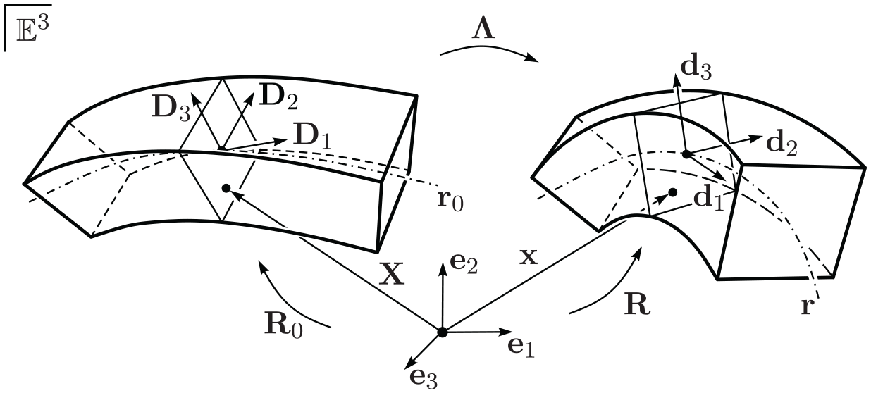
In this section, we introduce the required kinematical quantities required for the formulation of the spatial nonlinear Timoshenko beam, which is the least-constrained theory in this paper. The motion of the centerline is the mapping $\mathbf{r}:I\times \mathbb{R}\to {\mathbb{E}}^3,(\xi ,t)\mapsto \mathbf{r}(\xi ,t)$ , where, for each instant of time $t\in \mathbb{R}$ , the closed unit interval $I=[0,1]\subset \mathbb{R}$ parametrizes the set of beam points. The placement of the reference centerline is given by ${\mathbf{r}}_0:I\to {\mathbb{E}}^3$ . To capture cross-sectional orientations of beam-like bodies, the kinematics of the centerline is augmented by the motion of positively oriented director triads ${\mathbf{d}}_i:I\times \mathbb{R}\to {\mathbb{E}}^3$ . The directors ${\mathbf{d}}_{\alpha }(\xi ,t)$ span the plane and rigid cross section of the beam for the material coordinate $\xi$ at time $t$ . The director triads in the reference configuration are given by the mappings ${\mathbf{D}}_i:I\to {\mathbb{E}}^3$ . While ${\mathbf{D}}_1$ is identified with the unit tangent to the reference centerline ${\mathbf{r}}_0$ , i.e., ${\mathbf{D}}_1=\mathbf{r}{\prime }_0/\parallel \mathbf{r}{\prime }_0\parallel$ , the vectors ${\mathbf{D}}_2(\xi )$ and ${\mathbf{D}}_3(\xi )$ are identified with the geometric principal axes of the cross sections, see Figure 1.

Figure 1.

Kinematics of the Timoshenko beam’s reference and current placement.

With the reference and current rotation fields ${\mathbf{R}}_0:I\to \mathrm{Ort}{h}^{+}$ and $\mathbf{R}:I\times \mathbb{R}\to \mathrm{Ort}{h}^{+}$ , respectively, the reference and current director triads are related to a fixed right-handed inertial frame $\{{\mathbf{e}}_1,{\mathbf{e}}_2,{\mathbf{e}}_3\}$ by

$$\begin{array}{c}{\mathbf{D}}_i(\xi )={\mathbf{R}}_0(\xi ){\mathbf{e}}_i,{\mathbf{d}}_i(\xi ,t)=\mathbf{R}(\xi ,t){\mathbf{e}}_i,\hfill \\ {\mathbf{R}}_0(\xi )={\mathbf{D}}_i(\xi )\otimes {\mathbf{e}}_i,\mathbf{R}(\xi ,t)={\mathbf{d}}_i(\xi ,t)\otimes {\mathbf{e}}_i.\hfill \end{array}$$

(1)

By making use of the inverse relations of (1) and exploiting the equivalence of the inverse and the transpose for rotations, we can relate all bases by

$${\mathbf{e}}_i={\mathbf{R}}_0^{\mathrm{T}}(\xi ){\mathbf{D}}_i(\xi )={\mathbf{R}}^{\mathrm{T}}(\xi ,t){\mathbf{d}}_i(\xi ,t).$$

(2)

To capture the deformation between the reference and the current configuration, the rotation field $\mathbf{\Lambda }:I\times \mathbb{R}\to \mathrm{Ort}{h}^{+},(\xi ,t)\mapsto \mathbf{\Lambda }(\xi ,t)=\mathbf{R}(\xi ,t){\mathbf{R}}_0(\xi {)}^{\mathrm{T}}$ is introduced. It rotates the reference director triads to the current ones, i.e.,

$${\mathbf{d}}_i(\xi ,t)=\mathbf{\Lambda }(\xi ,t){\mathbf{D}}_i(\xi ),\mathbf{\Lambda }(\xi ,t)={\mathbf{d}}_i(\xi ,t)\otimes {\mathbf{D}}_i(\xi ).$$

The rate of change of the current directors with respect to time $t$ is described by the angular velocity $\tilde{\mathit{\omega }}(\xi ,t)=\stackrel{·}{\mathbf{R}}(\xi ,t){\mathbf{R}}^{\mathrm{T}}(\xi ,t)=\stackrel{·}{\mathbf{\Lambda }}(\xi ,t){\mathbf{\Lambda }}^{\mathrm{T}}(\xi ,t)\in \mathrm{Skw}$ , which appears together with the corresponding axial vector $\mathit{\omega }(\xi ,t)\in {\mathbb{E}}^3$ in

$${\stackrel{·}{\mathbf{d}}}_i=(\mathbf{R}{\mathbf{e}}_i{)}^{.}=\stackrel{·}{\mathbf{R}}{\mathbf{e}}_i\stackrel{(2)}{=}\stackrel{·}{\mathbf{R}}{\mathbf{R}}^{\mathrm{T}}{\mathbf{d}}_i=\tilde{\mathit{\omega }}{\mathbf{d}}_i=\mathit{\omega }\times {\mathbf{d}}_i.$$

(3)

The angular velocity can thus be represented as

$$\tilde{\mathit{\omega }}={\tilde{\omega }}_{\mathrm{ij}}{\mathbf{d}}_i\otimes {\mathbf{d}}_j=({\mathbf{d}}_i\otimes {\mathbf{e}}_i).({\mathbf{d}}_j\otimes {\mathbf{e}}_j{)}^{\mathrm{T}}={\stackrel{·}{\mathbf{d}}}_i\otimes {\mathbf{d}}_i=({\mathbf{d}}_i·{\stackrel{·}{\mathbf{d}}}_j){\mathbf{d}}_i\otimes {\mathbf{d}}_j$$

(4)

or as vector-valued function in the form

$$\mathit{\omega }={\omega }_i{\mathbf{d}}_i=\mathrm{ax}(\tilde{\mathit{\omega }})=\frac{1}{2}{\epsilon }_{\mathrm{ijk}}{\tilde{\omega }}_{\mathrm{kj}}{\mathbf{d}}_i=\frac{1}{2}{\epsilon }_{\mathrm{ijk}}({\mathbf{d}}_k·{\stackrel{·}{\mathbf{d}}}_j){\mathbf{d}}_i.$$

The rate of change of the current directors subjected to a variation of the current configuration is captured by the virtual rotation $\delta \tilde{\mathit{\varphi }}(\xi ,t)=\delta \mathbf{R}(\xi ,t){\mathbf{R}}^{\mathrm{T}}(\xi ,t)=\delta \mathbf{\Lambda }(\xi ,t){\mathbf{\Lambda }}^{\mathrm{T}}(\xi ,t)\in \mathrm{Skw}$ with its axial vector $\delta \mathit{\varphi }(\xi ,t)\in {\mathbb{E}}^3$ . Both representations can be recognized in

$$\delta {\mathbf{d}}_i=\delta \mathbf{R}{\mathbf{e}}_i\stackrel{(2)}{=}\delta \mathbf{R}{\mathbf{R}}^{\mathrm{T}}{\mathbf{d}}_i=\delta \tilde{\mathit{\varphi }}{\mathbf{d}}_i=\delta \mathit{\varphi }\times {\mathbf{d}}_i,$$

which implies the relation

$${\mathbf{d}}_i\times \delta {\mathbf{d}}_i={\mathbf{d}}_i\times (\delta \mathit{\varphi }\times {\mathbf{d}}_i)=({\mathbf{d}}_i·{\mathbf{d}}_i)\delta \mathit{\varphi }-({\mathbf{d}}_i·\delta \mathit{\varphi }){\mathbf{d}}_i=3\delta \mathit{\varphi }-\delta \mathit{\varphi }=2\delta \mathit{\varphi },$$

where Grassmann’s identity was used for the second equality. Thus, the virtual rotation $\delta \mathit{\varphi }$ and its first derivative $\delta \mathit{\varphi }\prime$ with respect to the beams material coordinate can be written as

$$\delta \mathit{\varphi }=\frac{1}{2}{\mathbf{d}}_i\times \delta {\mathbf{d}}_i,\delta \mathit{\varphi }\prime =\frac{1}{2}({\mathbf{d}\mathbf{\text{'}}}_i\times \delta {\mathbf{d}}_i+{\mathbf{d}}_i\times \delta {\mathbf{d}\mathbf{\text{'}}}_i).$$

(5)

2.3. Arc length parametrization

Let $\phi :\overline{I}=[l_1,l_2]\to I$ be the map from the domain of the arc length parameter of the reference centerline to the parameter domain $I$ and let ${\phi }^{-1}:I\to \overline{I}$ be the inverse mapping. Then, the arc length coordinate $s$ of the reference centerline at $\xi$ is defined as

$$s={\phi }^{-1}(\xi )={\int }_0^{\xi }\parallel {\mathbf{r}\mathbf{\text{'}}}_0(\overline{\xi })\parallel \mathrm{d}\overline{\xi }.$$

(6)

By differentiating the parameter integral with respect to $\xi$ using Leibniz’s rule and by exploiting the inverse function theorem, we can define

$$J(\xi ):=\parallel {\mathbf{r}\mathbf{\text{'}}}_0(\xi )\parallel =\frac{\partial {\phi }^{-1}}{\partial \xi }(\xi )=\frac{1}{\frac{\partial \phi }{\partial s}({\phi }^{-1}(\xi ))}.$$

(7)

Using (6) and (7), the respective differential measures $\mathrm{d}s$ and $\mathrm{d}\xi$ of the arc length and the parameter domain can be related by $\mathrm{d}s=J(\xi )\mathrm{d}\xi$ . Let $f$ be an arbitrary mapping $f:I\times \mathbb{R}\to {\mathbb{E}}^3$ , $(\xi ,t)\mapsto f(\xi ,t)$ , e.g., the beam’s current centerline, its derivative with respect to the arc length of the reference centerline is

$$\frac{\partial f}{\partial s}(\phi (s),t)=\frac{\partial f}{\partial \xi }(\phi (s),t)\frac{\partial \phi }{\partial s}(s)=\frac{\partial f}{\partial \xi }(\phi (s),t)\frac{1}{J(\phi (s))}.$$

Substituting $s={\phi }^{-1}(\xi )$ in the arguments and recognizing the identity map $\xi =\phi ({\phi }^{-1}(\xi ))$ , the derivative of a function defined in the parameter space $I$ with respect to the arc length parameter $s$ can therefore be defined as

$$\frac{\partial f}{\partial s}(\xi ,t):=\frac{\partial f}{\partial \xi }(\xi ,t)\frac{1}{J(\xi )}.$$

2.4. Strain energy, strain measures, and internal virtual work

Let the total strain energy stored in the beam be

$$E={\int }_{I}U(\xi ,t)J(\xi )\mathrm{d}[\xi ].$$

(8)

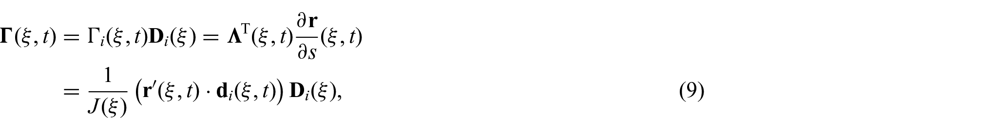
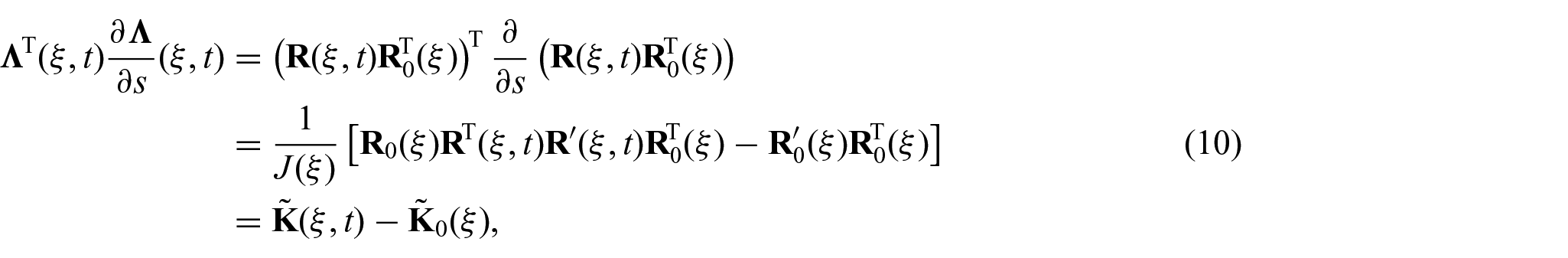
The chosen integral measure $J\mathrm{d}\xi$ enables the usage of SI units in the explicit formulation of strain energy densities. Therefore, $U$ has units $[\mathrm{J}/\mathrm{m}]$ , independent of the chosen parameter $\xi$ , which could possibly represent, for instance, the angle of an arch. Referring to [1, 31], an objective strain energy function, i.e., a function that is invariant under superimposed rigid-body motions or under the change of observer, must only depend on the subsequent two quantities

$$\begin{array}{c}\mathbf{\Gamma }(\xi ,t)={\mathrm{\Gamma }}_i(\xi ,t){\mathbf{D}}_i(\xi )={\mathbf{\Lambda }}^{\mathrm{T}}(\xi ,t)\frac{\partial \mathbf{r}}{\partial s}(\xi ,t)\hfill \\ =\frac{1}{J(\xi )}(\mathbf{r}\mathbf{\text{'}}(\xi ,t)·{\mathbf{d}}_i(\xi ,t)){\mathbf{D}}_i(\xi ),\hfill \end{array}$$

(9)

$$\begin{array}{c}{\mathbf{\Lambda }}^{\mathrm{T}}(\xi ,t)\frac{\partial \mathbf{\Lambda }}{\partial s}(\xi ,t)={(\mathbf{R}(\xi ,t){\mathbf{R}}_0^{\mathrm{T}}(\xi ))}^{\mathrm{T}}\frac{\partial }{\partial s}(\mathbf{R}(\xi ,t){\mathbf{R}}_0^{\mathrm{T}}(\xi ))\hfill \\ =\frac{1}{J(\xi )}[{\mathbf{R}}_0(\xi ){\mathbf{R}}^{\mathrm{T}}(\xi ,t)\mathbf{R}\mathbf{\text{'}}(\xi ,t){\mathbf{R}}_0^{\mathrm{T}}(\xi )-{\mathbf{R}\mathbf{\text{'}}}_0(\xi ){\mathbf{R}}_0^{\mathrm{T}}(\xi )]\hfill \\ =\tilde{\mathbf{K}}(\xi ,t)-{\tilde{\mathbf{K}}}_0(\xi ),\hfill \end{array}$$

(10)

where for the penultimate equality, the skew symmetry ${\mathbf{R}}_0{{\mathbf{R}\mathbf{\text{'}}}_0}^{\mathrm{T}}=-({\mathbf{R}}_0{{\mathbf{R}\mathbf{\text{'}}}_0}^{\mathrm{T}}{)}^{\mathrm{T}}=-{\mathbf{R}\mathbf{\text{'}}}_0{\mathbf{R}}_0^{\mathrm{T}}$ has been used. Inserting (1) into (10), we obtain the current curvatures

$$\tilde{\mathbf{K}}={\tilde{\mathrm{K}}}_{\mathrm{kj}}{\mathbf{D}}_k\otimes {\mathbf{D}}_j\mathrm{with}{\tilde{\mathrm{K}}}_{\mathrm{kj}}=\frac{{\mathbf{d}}_k·{\mathbf{d}\mathbf{\text{'}}}_j}{J},$$

and the reference curvatures

$${\tilde{\mathbf{K}}}_0={\tilde{\mathrm{K}}}_{\mathrm{kj}}^0{\mathbf{D}}_k\otimes {\mathbf{D}}_j\mathrm{with}{\tilde{\mathrm{K}}}_{\mathrm{kj}}^0=\frac{{\mathbf{D}}_k·{\mathbf{D}\mathbf{\text{'}}}_j}{J}.$$

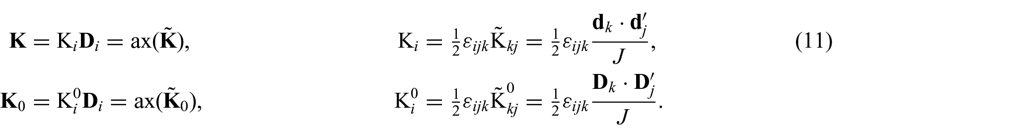
It can easily be verified that both $\tilde{\mathbf{K}}$ and ${\tilde{\mathbf{K}}}_0$ are skew symmetric and, hence, their associated axial vectors can be computed as

$$\begin{array}{c}\mathbf{K}={\mathrm{K}}_i{\mathbf{D}}_i=\mathrm{ax}(\tilde{\mathbf{K}}),{\mathrm{K}}_i=\frac{1}{2}{\epsilon }_{\mathrm{ijk}}{\tilde{\mathrm{K}}}_{\mathrm{kj}}=\frac{1}{2}{\epsilon }_{\mathrm{ijk}}\frac{{\mathbf{d}}_k·{\mathbf{d}\mathbf{\text{'}}}_j}{J},\hfill \\ {\mathbf{K}}_0={\mathrm{K}}_i^0{\mathbf{D}}_i=\mathrm{ax}({\tilde{\mathbf{K}}}_0),{\mathrm{K}}_i^0=\frac{1}{2}{\epsilon }_{\mathrm{ijk}}{\tilde{\mathrm{K}}}_{\mathrm{kj}}^0=\frac{1}{2}{\epsilon }_{\mathrm{ijk}}\frac{{\mathbf{D}}_k·{\mathbf{D}\mathbf{\text{'}}}_j}{J}.\hfill \end{array}$$

(11)

The previously introduced material strain measures $\mathbf{\Gamma }$ and $\mathbf{K}$ can be associated with their corresponding spatial strain measures by

$$\mathbf{\gamma }=\mathbf{\Lambda }\mathbf{\Gamma }={\mathrm{\Gamma }}_i{\mathbf{d}}_i,\mathit{\kappa }=\mathbf{\Lambda }\mathbf{K}={\mathrm{K}}_i{\mathbf{d}}_i,$$

where it should be noted that only the basis has changed but the components remain the same. An interpretation of the strain variables is given in [8, Section 6, p. 285]. Accordingly, ${\mathrm{\Gamma }}_1$ measures dilatation, i.e., the ratio of deformed to reference volume, ${\mathrm{\Gamma }}_2$ and ${\mathrm{\Gamma }}_3$ measure shear. Furthermore, ${\mathrm{K}}_1$ measures torsion, i.e., the amount of twist. ${\mathrm{K}}_2$ and ${\mathrm{K}}_3$ measure flexure, which does not coincide with the beam’s curvature. Moreover, $\lambda (\xi ,t)=\parallel \mathbf{\Gamma }(\xi ,t)\parallel$ is called the stretch.

For hyperelastic materials the objective strain energy function is of the form $U(\xi ,t)=W({\mathrm{\Gamma }}_i(\xi ,t),{\mathrm{K}}_i(\xi ,t);\xi )$ , solely depending on the given strain measures introduced above and possibly explicitly on the material point $\xi$ . Using the constitutive relations

$$n_i(\xi ,t)=\frac{\partial W}{\partial {\mathrm{\Gamma }}_i}({\mathrm{\Gamma }}_i(\xi ,t),{\mathrm{K}}_i(\xi ,t);\xi ),m_i(\xi ,t)=\frac{\partial W}{\partial {\mathrm{K}}_i}({\mathrm{\Gamma }}_i(\xi ,t),{\mathrm{K}}_i(\xi ,t);\xi ),$$

(12)

the material form of the generalized internal forces $\mathbf{N}=n_i{\mathbf{D}}_i$ and $\mathbf{M}=m_i{\mathbf{D}}_i$ can be identified. The analogous spatial form is obtained by $\mathbf{n}=\mathbf{\Lambda }\mathbf{N}=n_i{\mathbf{d}}_i$ and $\mathbf{m}=\mathbf{\Lambda }\mathbf{M}=m_i{\mathbf{d}}_i$ , which can be interpreted as resultant contact forces and moments, see [1,6,32]. Using the beam’s total internal energy (8), we define the internal virtual work contribution by

$$\delta W^{\mathrm{int}}=-\delta E=-{\int }_I\delta \mathrm{UJ}\mathrm{d}[\xi ]=-{\int }_I\{n_i\delta {\mathrm{\Gamma }}_i+m_i\delta {\mathrm{K}}_i\}J\mathrm{d}\xi .$$

(13)

Computing the variation of the objective strain measures (9) and (11), i.e.,

$$\delta {\mathrm{\Gamma }}_i=\frac{1}{J}(\delta \mathbf{r}\mathbf{\text{'}}·{\mathbf{d}}_i+\delta {\mathbf{d}}_i·\mathbf{r}\mathbf{\text{'}}),\delta {\mathrm{K}}_i=\frac{1}{2J}{\epsilon }_{\mathrm{ijk}}(\delta {\mathbf{d}}_k·{\mathbf{d}\mathbf{\text{'}}}_j+\delta {\mathbf{d}\mathbf{\text{'}}}_j·{\mathbf{d}}_k),$$

and inserting them into the internal virtual work, we obtain

$$\delta W^{\mathrm{int}}=-{\int }_I\{\delta \mathbf{r}\mathbf{\text{'}}·n_i{\mathbf{d}}_i+\delta {\mathbf{d}}_i·(n_i\mathbf{r}\mathbf{\text{'}}+{\epsilon }_{\mathrm{kji}}\frac{m_k}{2}{\mathbf{d}\mathbf{\text{'}}}_j)+\delta {\mathbf{d}\mathbf{\text{'}}}_j·{\epsilon }_{\mathrm{ijk}}\frac{m_i}{2}{\mathbf{d}}_k\}\mathrm{d}\xi ,$$

(14)

which is in accordance with the derivations given in [4]. Note that even in the inelastic case, where no strain energy function is available, the internal virtual work (14) can be used, where the components of the generalized internal forces $n_i$ and $m_i$ are defined by different constitutive laws. Unless stated otherwise, subsequently, we use a hyperelastic material model defined by the nonlinear ¹ strain energy density

$$\begin{array}{c}U(\xi ,t)=\frac{1}{2}{E}_1(\xi ){[\lambda (\xi ,t)-1]}^2+\frac{1}{2}{E}_{\alpha }(\xi ){[{\mathrm{\Gamma }}_{\alpha }(\xi ,t)-{\mathrm{\Gamma }}_{\alpha }^0(\xi )]}^2\hfill \\ +\frac{1}{2}{F}_i(\xi ){[{\mathrm{K}}_i(\xi ,t)-{\mathrm{K}}_i^0(\xi )]}^2,\hfill \end{array}$$

(15)

where ${\mathrm{\Gamma }}_{\alpha }^0={\mathbf{D}}_{\alpha }·{\mathbf{r}}_0^{\prime }$ denote the shear strains in the reference configuration.

2.5. External virtual work and inertia contributions

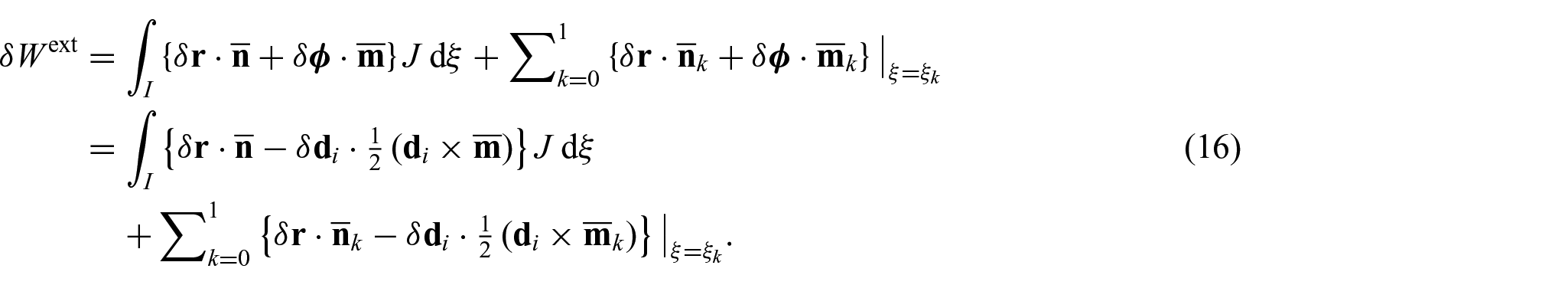
As shown in [1], the beam can be subjected to distributed external forces $\overline{\mathbf{n}}:I\times \mathbb{R}\to {\mathbb{E}}^3$ and distributed external couples $\overline{\mathbf{m}}:I\times \mathbb{R}\to {\mathbb{E}}^3$ . In addition, we allow point-wise defined external forces ${\overline{\mathbf{n}}}_0,{\overline{\mathbf{n}}}_1:\mathbb{R}\to {\mathbb{E}}^3$ and couples ${\overline{\mathbf{m}}}_0,{\overline{\mathbf{m}}}_1:\mathbb{R}\to {\mathbb{E}}^3$ to be applied on the boundaries ${\xi }_0=0$ and ${\xi }_1=1$ of the beam. Using (5) together with the invariance of the triple product, the virtual work contributions of the external forces take the form

$$\begin{array}{c}\delta W^{\mathrm{ext}}={\int }_I\{\delta \mathbf{r}·\overline{\mathbf{n}}+\delta \mathit{\varphi }·\overline{\mathbf{m}}\}J\mathrm{d}[\xi ]+{\sum }_{k=0}^1\{\delta \mathbf{r}·{\overline{\mathbf{n}}}_k+\delta \mathit{\varphi }·{\overline{\mathbf{m}}}_k\}{|}_{\xi ={\xi }_k}\hfill \\ ={\int }_I\{\delta \mathbf{r}·\overline{\mathbf{n}}-\delta {\mathbf{d}}_i·\frac{1}{2}({\mathbf{d}}_i\times \overline{\mathbf{m}})\}J\mathrm{d}\xi \hfill \\ +{\sum }_{k=0}^1\{\delta \mathbf{r}·{\overline{\mathbf{n}}}_k-\delta {\mathbf{d}}_i·\frac{1}{2}({\mathbf{d}}_i\times {\overline{\mathbf{m}}}_k)\}{|}_{\xi ={\xi }_k}.\hfill \end{array}$$

(16)

Note that the used integral measure $J\mathrm{d}\xi$ enables the specification of the external distributed forces $\overline{\mathbf{n}}$ and couples $\overline{\mathbf{m}}$ in the convenient units $[\mathrm{N}/\mathrm{m}]$ and $[\mathrm{Nm}/\mathrm{m}]$ , respectively, where both are parametrized by $\xi \in I$ .

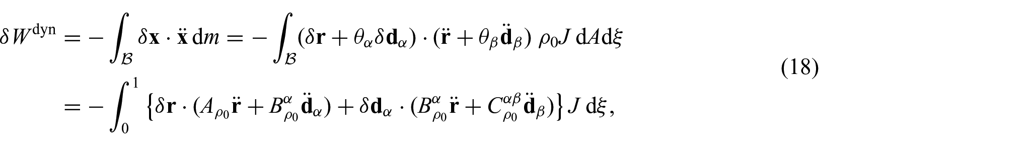
In order to formulate the virtual work contributions of inertia effects, we assume the beam to be a three-dimensional continuous body whose points in the reference configuration occupy the positions

$$\mathbf{X}(\xi ,{\theta }_{\alpha })={\mathbf{r}}_0(\xi )+{\theta }_{\alpha }{\mathbf{D}}_{\alpha }(\xi ).$$

Hence, every material point in the reference configuration is addressed by the coordinates $(\xi ,{\theta }_2,{\theta }_3)\in \mathcal{B}\subset {\mathbb{R}}^3$ . We assume that the cross sections of the beam are spanned by the reference directors ${\mathbf{D}}_2$ and ${\mathbf{D}}_3$ such that ${\theta }_2$ and ${\theta }_3$ are the cross-section coordinates. In the sense of an induced theory, see [33], we assume the beam to be a constrained three-dimensional continuum whose current configuration is restricted to

$$\mathbf{x}(\xi ,{\theta }_{\alpha },t)=\mathbf{r}(\xi ,t)+{\theta }_{\alpha }{\mathbf{d}}_{\alpha }(\xi ,t).$$

(17)

In fact the kinematical ansatz (17) restricts the motion of the cross sections such that they have to remain plane and rigid for any motion. Next, the beam’s mass density per unit volume in its reference configuration ${\rho }_0:\mathcal{B}\to \mathbb{R}$ and the cross-sectional surface element in the beam’s reference configuration $\mathrm{d}A$ can be introduced. In order to express the beam’s density ${\rho }_0(\xi )$ in the convenient unit $[\mathrm{kg}/{\mathrm{m}}^3]$ parametrized by $\xi \in I$ the mass differential is defined as $\mathrm{d}m={\rho }_{0}J\mathrm{d}A\mathrm{d}\xi$ in accordance with the beam’s total mass $M={\int }_{\mathcal{B}}\mathrm{d}m$ . The virtual work of the inertia forces of a three-dimensional continuum is commonly defined as

$$\begin{array}{c}\delta W^{\mathrm{dyn}}=-{\int }_{\mathcal{B}}\delta \mathbf{x}·\stackrel{··}{\mathbf{x}}\mathrm{d}m=-{\int }_{\mathcal{B}}(\delta \mathbf{r}+{\theta }_{\alpha }\delta {\mathbf{d}}_{\alpha })·(\stackrel{··}{\mathbf{r}}+{\theta }_{\beta }{\stackrel{··}{\mathbf{d}}}_{\beta }){\rho }_{0}J\mathrm{d}A\mathrm{d}\xi \hfill \\ =-{\int }_0^1\{\delta \mathbf{r}·(A_{{\rho }_0}\stackrel{··}{\mathbf{r}}+B_{{\rho }_0}^{\alpha }{\stackrel{··}{\mathbf{d}}}_{\alpha })+\delta {\mathbf{d}}_{\alpha }·(B_{{\rho }_0}^{\alpha }\stackrel{··}{\mathbf{r}}+C_{{\rho }_0}^{\alpha \beta }{\stackrel{··}{\mathbf{d}}}_{\beta })\}J\mathrm{d}\xi ,\hfill \end{array}$$

(18)

where the integrated quantities ²

$$A_{{\rho }_0}(\xi )={\int }_{A(\xi )}{\rho }_0(\xi )\mathrm{d}A,B_{{\rho }_0}^{\alpha }(\xi )={\int }_{A(\xi )}{\rho }_0(\xi ){\theta }_{\alpha }\mathrm{d}A,C_{{\rho }_0}^{\alpha \beta }(\xi )={\int }_{A(\xi )}{\rho }_0(\xi ){\theta }_{\alpha }{\theta }_{\beta }\mathrm{d}A$$

(19)

have been introduced.

2.6. Constraint virtual work

Next, at each material point $\xi$ and at each instant of time $t$ additionally $m$ holonomic scleronomic constraint equations, possibly depending on the kinematic quantities $\mathbf{r}$ and ${\mathbf{d}}_i$ and their first derivatives, have to be fulfilled

$$g_k(\xi ,t)=g_k(\mathbf{r}(\xi ,t),\mathbf{r}\mathbf{\text{'}}(\xi ,t),{\mathbf{d}}_i(\xi ,t),{\mathbf{d}\mathbf{\text{'}}}_i(\xi ,t)),k=1,\dots ,m,\forall \xi ,\forall t.$$

(20)

For the director beam formulation the requirement of $\mathbf{R}={\mathbf{d}}_i\otimes {\mathbf{e}}_i$ being a proper rotation, i.e., the directors must remain orthonormal throughout the motion of the beam. This leads to six independent constraint equations

$$g_{\mathrm{ij}}(\xi ,t)={\mathbf{d}}_i(\xi ,t)·{\mathbf{d}}_j(\xi ,t)-{\delta }_{\mathrm{ij}}=0,1\le i\le j\le 3,$$

(21)

the corresponding index $k=4,\dots ,9$ for the identification of $g_k$ is given by the mapping $P:(11,12,13,22,23,33)\to (4,5,6,7,8,9)$ .

In addition, if the director ${\mathbf{d}}_1$ is constrained to align with the centerline’s tangent, we call the beam an Euler–Bernoulli beam [1, 34, 35]. This can be ensured by the constraint equations

$$g_{\alpha }(\xi ,t)={\mathrm{\Gamma }}_{\alpha }(\xi ,t)={\mathbf{d}}_{\alpha }(\xi ,t)·\mathbf{r}\mathbf{\text{'}}(\xi ,t)=0,\alpha =2,3,$$

(22)

which coincides with vanishing shear strains.

If further the length of the centerline’s tangent remains unchanged throughout the motion, i.e., dilatation is restricted, an inextensible Euler–Bernoulli beam is obtained by enforcing the constraint

$$g_1(\xi ,t)={\mathrm{\Gamma }}_1(\xi ,t)-1={\mathbf{d}}_1(\xi ,t)·\mathbf{r}\mathbf{\text{'}}(\xi ,t)-1=0.$$

(23)

As ${\mathbf{d}}_{\alpha }·\mathbf{r}\mathbf{\text{'}}=0$ and by assuming for physical reasonable situations ${\mathbf{d}}_1·\mathbf{r}\mathbf{\text{'}}>0$ it can be shown that (23) coincides with the centerline’s tangent being of unit length [1], i.e., $g_1=\parallel \mathbf{r}\mathbf{\text{'}}\parallel -1=0$ .

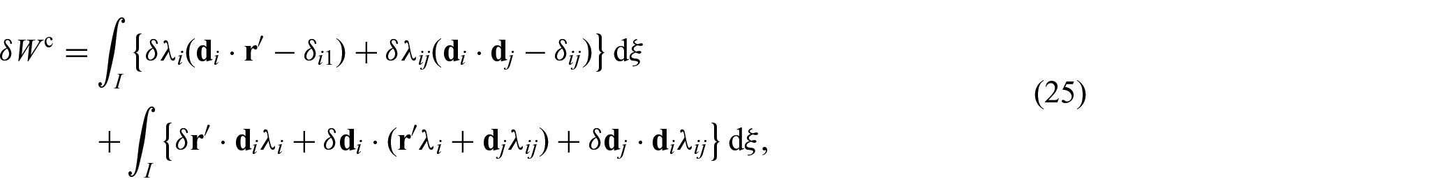
By introducing the Lagrange multiplier fields ${\lambda }_k:I\times \mathbb{R}\to \mathbb{R}$ , $k=1,\dots ,m$ , and demanding the constraint equations (20) to hold in a weak sense, the virtual work contribution of the $m$ perfect bilateral constraints is

$$\delta W^{\mathrm{c}}=\delta {\int }_I{g}_k(\xi ,t){\lambda }_k(\xi ,t)\mathrm{d}\xi ={\int }_I{g}_k(\xi ,t)\delta {\lambda }_k(\xi ,t)\mathrm{d}\xi +{\int }_I\delta g_k(\xi ,t){\lambda }_k(\xi ,t)\mathrm{d}\xi ,$$

(24)

which can be decomposed into two parts, the first one being the weak form of the constraint conditions and the second one corresponding to the virtual work of the constraint forces. The above introduced constraint equations (21), (22), and (23) together with their variations can be summarized as follows:

$$\begin{array}{c}{g}_i={\mathbf{d}}_i·\mathbf{r}\mathbf{\text{'}}-{\delta }_{i1},g_{\mathrm{ij}}={\mathbf{d}}_i·{\mathbf{d}}_j-{\delta }_{\mathrm{ij}},\hfill \\ \multicolumn{1}{c}{\delta g_i=\delta {\mathbf{d}}_i·\mathbf{r}\mathbf{\text{'}}+\delta \mathbf{r}\mathbf{\text{'}}·{\mathbf{d}}_i,\delta g_{\mathrm{ij}}=\delta {\mathbf{d}}_i·{\mathbf{d}}_j+\delta {\mathbf{d}}_j·{\mathbf{d}}_i.}\end{array}$$

Thus, by substituting these equations into (24), the virtual work contribution of the constraints is

$$\begin{array}{c}\delta W^{\mathrm{c}}={\int }_I\{\delta {\lambda }_i({\mathbf{d}}_i·\mathbf{r}\mathbf{\text{'}}-{\delta }_{i1})+\delta {\lambda }_{\mathrm{ij}}({\mathbf{d}}_i·{\mathbf{d}}_j-{\delta }_{\mathrm{ij}})\}\mathrm{d}\xi \hfill \\ +{\int }_I\{\delta \mathbf{r}\mathbf{\text{'}}·{\mathbf{d}}_i{\lambda }_i+\delta {\mathbf{d}}_i·(\mathbf{r}\mathbf{\text{'}}{\lambda }_i+{\mathbf{d}}_j{\lambda }_{\mathrm{ij}})+\delta {\mathbf{d}}_j·{\mathbf{d}}_i{\lambda }_{\mathrm{ij}}\}\mathrm{d}\xi ,\hfill \end{array}$$

(25)

where the terms involving a double subscript are summed over the indices $1\le i\le j\le 3$ . The corresponding index $k=4,\dots ,9$ for the identification of ${\lambda }_k$ and $\delta {\lambda }_k$ is also given by the previously introduced mapping $P$ . The mathematically rigorous question about the Lagrange multipliers’ correct functional spaces and their approximations must be answered with much care and we only refer to [36, 37] for further reading on that topic. However, with many benchmark examples, we give in Section 4 numerical evidence of a well-chosen approximation of the Lagrange multiplier fields.

2.7. Principle of virtual work

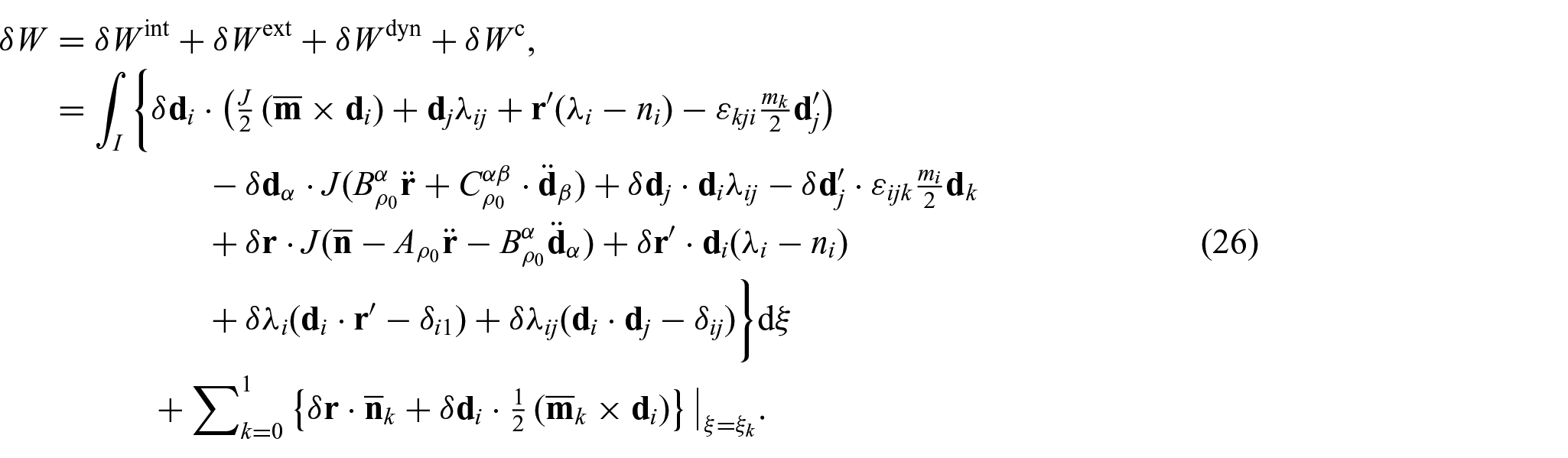
The total virtual work is obtained by summing up all the virtual work contributions, consisting of the internal (14), external (16), inertia (18), and constraint contributions (25), i.e.,

$$\begin{array}{c}\delta W=\delta W^{\mathrm{int}}+\delta W^{\mathrm{ext}}+\delta W^{\mathrm{dyn}}+\delta W^{\mathrm{c}},\hfill \\ ={\int }_I\{\delta {\mathbf{d}}_i·(\frac{J}{2}(\overline{\mathbf{m}}\times {\mathbf{d}}_i)+{\mathbf{d}}_j{\lambda }_{\mathrm{ij}}+\mathbf{r}\mathbf{\text{'}}({\lambda }_i-n_i)-{\epsilon }_{\mathrm{kji}}\frac{m_k}{2}{\mathbf{d}\mathbf{\text{'}}}_j)\hfill \\ -\delta {\mathbf{d}}_{\alpha }·J(B_{{\rho }_0}^{\alpha }\stackrel{··}{\mathbf{r}}+C_{{\rho }_0}^{\alpha \beta }·{\stackrel{··}{\mathbf{d}}}_{\beta })+\delta {\mathbf{d}}_j·{\mathbf{d}}_i{\lambda }_{\mathrm{ij}}-\delta {\mathbf{d}\mathbf{\text{'}}}_j·{\epsilon }_{\mathrm{ijk}}\frac{m_i}{2}{\mathbf{d}}_k\hfill \\ +\delta \mathbf{r}·J(\overline{\mathbf{n}}-A_{{\rho }_0}\stackrel{··}{\mathbf{r}}-B_{{\rho }_0}^{\alpha }{\stackrel{··}{\mathbf{d}}}_{\alpha })+\delta \mathbf{r}\mathbf{\text{'}}·{\mathbf{d}}_i({\lambda }_i-n_i)\hfill \\ +\delta {\lambda }_i({\mathbf{d}}_i·\mathbf{r}\mathbf{\text{'}}-{\delta }_{i1})+\delta {\lambda }_{\mathrm{ij}}({\mathbf{d}}_i·{\mathbf{d}}_j-{\delta }_{\mathrm{ij}})\}\mathrm{d}\xi \hfill \\ +{\sum }_{k=0}^1\{\delta \mathbf{r}·{\overline{\mathbf{n}}}_k+\delta {\mathbf{d}}_i·\frac{1}{2}({\overline{\mathbf{m}}}_k\times {\mathbf{d}}_i)\}{|}_{\xi ={\xi }_k}.\hfill \end{array}$$

(26)

Note, again terms involving a double subscript are summed over the indices $1\le i\le j\le 3$ . Moreover, the principle of virtual work states the body is in dynamic equilibrium if the total virtual work $\delta W$ vanishes for all virtual displacements $\delta \mathbf{r}$ , $\delta {\mathbf{d}}_i$ , $\delta {\lambda }_k$ at any instant of time $t$ .

2.8. Plane linearized director beam theory

In order to compare the new director beam formulation with the well-known planar Timoshenko beam formulation and to get a better understanding how it can be interpreted, we constrain the virtual work contributions for the static analysis to the plane and linearized case.

In the following, we assume small displacements of an initially straight beam. Then the kinematics, i.e., centerline and directors, in terms of the reference arc-length $s$ can be written as

$$\mathbf{r}(s,t)={\mathbf{r}}_0(s)+\mathbf{u}(s,t),{\mathbf{r}}_0(s)=s{\mathbf{e}}_1,{\mathbf{d}}_i(s,t)={\mathbf{e}}_i+{\mathbf{v}}_i(s,t).$$

Using in this section the prime to denote the derivative with respect to the arc-length parameter $s$ , we obtain

$$\mathbf{r}\mathbf{\text{'}}(s,t)={\mathbf{e}}_1+\mathbf{u}\mathbf{\text{'}}(s,t),{\mathbf{d}\mathbf{\text{'}}}_i(s,t)={\mathbf{v}\mathbf{\text{'}}}_i(s,t).$$

A planar motion is obtained by setting $\mathbf{u}=u_x{\mathbf{e}}_1+u_y{\mathbf{e}}_2$ , ${\mathbf{v}}_1=v_{1x}{\mathbf{e}}_1+v_{1y}{\mathbf{e}}_2$ , ${\mathbf{v}}_2=v_{2x}{\mathbf{e}}_1+v_{2y}{\mathbf{e}}_2$ and ${\mathbf{v}}_3=0$ . Considering the linearized theory, the assumptions $\parallel \mathbf{u}\mathbf{\text{'}}\parallel <<1$ and $\parallel {\mathbf{v}}_i\parallel <<1$ have to hold. With the kinematic assumptions introduced previously, the axial and shear strains (9) reduce to

$${\mathrm{\Gamma }}_1=1+{\mathbf{v}}_1·{\mathbf{e}}_1+\mathbf{u}\mathbf{\text{'}}·{\mathbf{e}}_1,{\mathrm{\Gamma }}_2={\mathbf{v}}_2·{\mathbf{e}}_1+\mathbf{u}\mathbf{\text{'}}·{\mathbf{e}}_2,{\mathrm{\Gamma }}_3=0,$$

where the terms $\mathbf{u}\mathbf{\text{'}}·{\mathbf{v}}_i$ were assumed to be negligibly small. Accordingly, by assuming ${\mathbf{v}}_2·{\mathbf{v}\mathbf{\text{'}}}_1$ and ${\mathbf{v}\mathbf{\text{'}}}_2·{\mathbf{v}}_1$ to be negligibly small, the torsional and flexural strain measures (11) are reduced to

$${\mathrm{K}}_1={\mathrm{K}}_2=0,{\mathrm{K}}_3=\frac{1}{2}({\mathbf{v}\mathbf{\text{'}}}_1·{\mathbf{e}}_2-{\mathbf{v}\mathbf{\text{'}}}_2·{\mathbf{e}}_1).$$

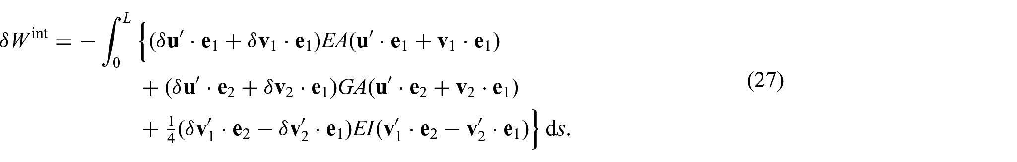
By computing the variation of the non-vanishing linearized strain measures

$$\delta {\mathrm{\Gamma }}_1=\delta \mathbf{u}\mathbf{\text{'}}·{\mathbf{e}}_1+\delta {\mathbf{v}}_1·{\mathbf{e}}_1,\delta {\mathrm{\Gamma }}_2=\delta \mathbf{u}\mathbf{\text{'}}·{\mathbf{e}}_2+\delta {\mathbf{v}}_2·{\mathbf{e}}_1,\delta {\mathrm{K}}_3=\frac{1}{2}(\delta {\mathbf{v}\mathbf{\text{'}}}_1·{\mathbf{e}}_2-\delta {\mathbf{v}\mathbf{\text{'}}}_2·{\mathbf{e}}_1)$$

and using linear elastic constitutive laws

$$n_1=\mathrm{EA}({\mathrm{\Gamma }}_1-1),n_2=\mathrm{GA}{\mathrm{\Gamma }}_2,n_3=m_1=m_2=0,m_3=\mathrm{EI}{\mathrm{K}}_3,$$

with Young’s modulus $E$ , shear modulus $G$ , cross-section area $A$ , and the second moment of area $I$ , the internal virtual work of the nonlinear spatial Timoshenko beam (13) reduces to

$$\begin{array}{c}\delta W^{\mathrm{int}}=-{\int }_0^L\{(\delta \mathbf{u}\mathbf{\text{'}}·{\mathbf{e}}_1+\delta {\mathbf{v}}_1·{\mathbf{e}}_1)\mathrm{EA}(\mathbf{u}\mathbf{\text{'}}·{\mathbf{e}}_1+{\mathbf{v}}_1·{\mathbf{e}}_1)\hfill \\ \multicolumn{1}{c}{+(\delta \mathbf{u}\mathbf{\text{'}}·{\mathbf{e}}_2+\delta {\mathbf{v}}_2·{\mathbf{e}}_1)\mathrm{GA}(\mathbf{u}\mathbf{\text{'}}·{\mathbf{e}}_2+{\mathbf{v}}_2·{\mathbf{e}}_1)}\\ \multicolumn{1}{c}{+\frac{1}{4}(\delta {\mathbf{v}\mathbf{\text{'}}}_1·{\mathbf{e}}_2-\delta {\mathbf{v}\mathbf{\text{'}}}_2·{\mathbf{e}}_1)\mathrm{EI}({\mathbf{v}\mathbf{\text{'}}}_1·{\mathbf{e}}_2-{\mathbf{v}\mathbf{\text{'}}}_2·{\mathbf{e}}_1)\}\mathrm{d}s.}\end{array}$$

(27)

It should be emphasized that the classical plane linearized Timoshenko beam theory can be deduced from the theory above by parameterizing the two directors using a single absolute angle $\theta$ with respect to the ${\mathbf{e}}_1$ -axis, i.e.,

$$\begin{array}{c}{\mathbf{d}}_1=\cos \theta {\mathbf{e}}_1+\sin \theta {\mathbf{e}}_2\Rightarrow {\mathbf{v}}_1={\mathbf{d}}_1-{\mathbf{e}}_1=(\cos \theta -1){\mathbf{e}}_1+\sin \theta {\mathbf{e}}_2,\hfill \\ \multicolumn{1}{c}{{\mathbf{d}}_2=\cos \theta {\mathbf{e}}_2-\sin \theta {\mathbf{e}}_1\Rightarrow {\mathbf{v}}_2={\mathbf{d}}_2-{\mathbf{e}}_2=(\cos \theta -1){\mathbf{e}}_2-\sin \theta {\mathbf{e}}_1.}\end{array}$$

(28)

Inserting (28) into the plane linearized internal virtual work (27) and after performing simple algebraic manipulations, together with the small angle assumptions $\cos \theta \approx 1$ , $\sin \theta \approx \theta$ , the well-known expression

$$\delta W^{\mathrm{int}}=-{\int }_0^L\{\delta u_{x\prime }\mathrm{EA}{u}_{x\prime }+(\delta u_{y\prime }-\delta \theta )\mathrm{GA}(u_{y\prime }-\theta )+\delta \theta \prime \mathrm{EI}\theta \prime \}\mathrm{d}s$$

(29)

is obtained.

In a similar manner as previously, the constraint equations ensuring the orthonormality conditions (21) can be linearized

$$\begin{array}{ccc}{g}_{11}=2{\mathbf{v}}_1·{\mathbf{e}}_1,\hfill & g_{22}=2{\mathbf{v}}_2·{\mathbf{e}}_2,\hfill & g_{12}={\mathbf{v}}_1·{\mathbf{e}}_2+{\mathbf{v}}_2·{\mathbf{e}}_2,\hfill \end{array}$$

(30)

where ${\mathbf{v}}_i·{\mathbf{v}}_j$ was assumed to be negligibly small and $g_{13}=g_{23}=g_{33}=0$ . The linearized orthonormality constraints (30) can be interpreted as the equations enforcing the directors to move as an infinitesimal rotation, i.e., ${\mathbf{v}}_1\perp {\mathbf{e}}_1$ , ${\mathbf{v}}_2\perp {\mathbf{e}}_2$ and ${\mathbf{v}}_1·{\mathbf{e}}_2=-{\mathbf{v}}_2·{\mathbf{e}}_2$ . The plane linearized version of the inextensibility (23) and the shear rigidity (22) can be summarized as

$$g_1={\mathrm{\Gamma }}_1-1=\mathbf{u}\mathbf{\text{'}}·{\mathbf{e}}_1+{\mathbf{v}}_1·{\mathbf{e}}_1,g_2={\mathrm{\Gamma }}_2={\mathbf{v}}_2·{\mathbf{e}}_1+\mathbf{u}\mathbf{\text{'}}·{\mathbf{e}}_2,g_3={\mathrm{\Gamma }}_3=0.$$

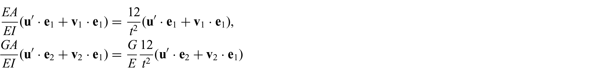
For simplicity, but without loss of generality, we assume a quadratic beam cross section with edges $t$ . This implies the cross-section area $A=t^2$ and the second moment of area $I=t^4/12$ . By dividing the plane linearized virtual work (27) by the constant $\mathrm{EI}$ two noteworthy terms

$$\begin{array}{c}\frac{\mathrm{EA}}{\mathrm{EI}}(\mathbf{u}\mathbf{\text{'}}·{\mathbf{e}}_1+{\mathbf{v}}_1·{\mathbf{e}}_1)=\frac{12}{t^2}(\mathbf{u}\mathbf{\text{'}}·{\mathbf{e}}_1+{\mathbf{v}}_1·{\mathbf{e}}_1),\hfill \\ \frac{\mathrm{GA}}{\mathrm{EI}}(\mathbf{u}\mathbf{\text{'}}·{\mathbf{e}}_2+{\mathbf{v}}_2·{\mathbf{e}}_1)=\frac{G}{E}\frac{12}{t^2}(\mathbf{u}\mathbf{\text{'}}·{\mathbf{e}}_2+{\mathbf{v}}_2·{\mathbf{e}}_1)\hfill \end{array}$$

appear. In the limit $t\to 0$ , the first term imposes the condition $\mathbf{u}\mathbf{\text{'}}·{\mathbf{e}}_1+{\mathbf{v}}_1·{\mathbf{e}}_1\to 0$ . When the first orthonormality constraint condition $g_{11}=2{\mathbf{v}}_1·{\mathbf{e}}_1$ is fulfilled, this reduces to the inextensibility condition $\mathbf{u}\mathbf{\text{'}}·{\mathbf{e}}_1=u_{x\prime }=0$ . The second term imposes the condition $\mathbf{u}\mathbf{\text{'}}·{\mathbf{e}}_2+{\mathbf{v}}_2·{\mathbf{e}}_1\to 0$ . This corresponds to the equality $u_{y\prime }=-v_{2x}$ . For the classical Timoshenko beam formulation (29) this corresponds to the constraint $u_{y\prime }=\theta$ . As noted by [38], this condition cannot be satisfied in general by numerical methods using equal order shape function approximations for $\mathbf{u}$ and ${\mathbf{v}}_i$ , which causes the locking effect in classical plane linearized Timoshenko beam formulations (not only in the limit $t\to 0$ but for small values of $t$ as well). Led by these observations, we expect the spatial nonlinear director beam formulation to suffer from the similar locking phenomenon for increasing slenderness when equal order shape functions are used to discretize $\mathbf{u}$ and ${\mathbf{v}}_i$ and in the nonlinear case $\mathbf{r}$ and ${\mathbf{d}}_i$ . Thus, in Section 4, appropriate polynomial degrees are chosen for discretizing the different fields.

3. Galerkin discretization

For the spatial discretization, all previously arising vector quantities will be expressed in the orthonormal basis $\{{\mathbf{e}}_1,{\mathbf{e}}_2,{\mathbf{e}}_3\}$ . For that, we collect the components of vectors $\mathbf{a}=a_1{\mathbf{e}}_1+a_2{\mathbf{e}}_2+a_3{\mathbf{e}}_3\in {\mathbb{E}}^3$ in the tuple ${}_I\mathbf{a}=(a_1,a_2,a_3{)}^{\mathrm{T}}\in {\mathbb{R}}^3$ . If not stated otherwise, ${\mathbb{R}}^f$ -tuples are considered in the sense of matrix multiplication as ${\mathbb{R}}^{f\times 1}$ -matrices, i.e., as “column vectors.” Its transposed will be given by a ${\mathbb{R}}^{1\times f}$ -matrix, i.e., a “row vector.” Further, partial derivatives of vector valued functions $f:{\mathbb{R}}^f\to \mathbb{R},\mathbf{q}\to f(\mathbf{q})$ , are introduced as “row vectors” $\partial f/\partial \mathbf{q}=(\partial f/\partial q^1\cdots \partial f/\partial q^f)\in {\mathbb{R}}^{1\times f}$ .

3.1. B-spline curves

The excellent monograph [39] gives a comprehensive introduction to the topic. They introduce B-spline shape functions and B-spline curves, together with a myriad of important properties. For the sake of simplicity, we restrict ourselves to knot vectors of the form

$${\mathbf{\Xi }}_{\square }=\{\underset{p_{\square }+1}{\underbrace{0,\dots ,0}},\underset{n-1}{\underbrace{\mathrm{\Delta }\xi ,,\dots ,e\mathrm{\Delta }\xi ,\dots ,(n-1)\mathrm{\Delta }\xi }},\underset{p_{\square }+1}{\underbrace{1,\dots ,1}}\},$$

where the box □ denotes a single kinematic quantity, e.g., the beam’s centerline $\mathbf{r}$ or one of the three directors ${\mathbf{d}}_i$ . Determined by the chosen polynomial degree $p_{\square }$ of the target B-spline curve and the total number $n$ of curve sections (also known as elements), such an open and uniform knot vector consists of a total number of $q_{\square }=n+2p_{\square }+1$ knots.

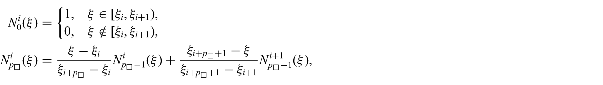
According to [39–41], the $i$ th of total $N_{\square }=n+p_{\square }$ B-spline shape functions is recursively defined as

$$\begin{array}{cc}{N}_0^i(\xi )\hfill & =(\begin{array}{cc}1,\hfill & \xi \in [{\xi }_i,{\xi }_{i+1}),\hfill \\ \multicolumn{1}{c}{0,}& \xi \notin [{\xi }_i,{\xi }_{i+1}),\hfill \end{array}\hfill \\ \multicolumn{1}{c}{N_{p_{\square }}^i(\xi )}& =\frac{\xi -{\xi }_i}{{\xi }_{i+p_{\square }}-{\xi }_i}{N}_{p_{\square }-1}^i(\xi )+\frac{{\xi }_{i+p_{\square }+1}-\xi }{{\xi }_{i+p_{\square }+1}-{\xi }_{i+1}}{N}_{p_{\square }-1}^{i+1}(\xi ),\hfill \end{array}$$

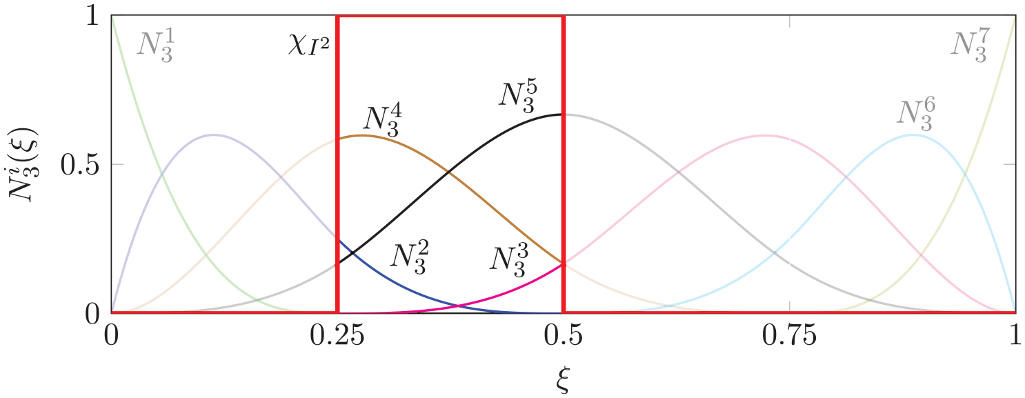
where in the last line possibly arising quotients of the form $\frac{0}{0}$ are defined as zero. In Figure 2 all non-zero cubic shape functions for a uniform open knot vector, built of four elements, are shown.

Figure 2.

Non-zero cubic B-spline shape functions $N_3^1$ to $N_3^7$ for a given uniform and open knot vector $\mathbf{\Xi }=\{0,0,0,0,0.25,0.5,0.75,1,1,1,1\}$ which builds $n=4$ elements. The indicator function ${\chi }_{I^2}$ of the second element selects the corresponding cubic shape functions $N_3^2$ to $N_3^5$ .

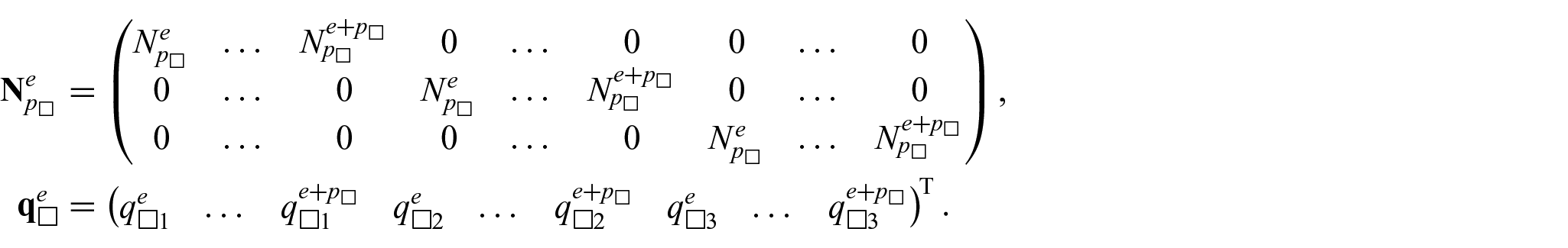
The Cartesian components of the beam’s kinematic quantities can be approximated by a $p_{\square }$ th degree B-spline curve of the form

$${}_I\square (\xi ,t)={\sum }_{e=1}^n{\chi }_{I^e}(\xi ){\mathbf{N}}_{p_{\square }}^e(\xi ){\mathbf{q}}_{\square }^e(t),$$

where ${\chi }_{I^e}:I\to \{0,1\}$ is the standard indicator function being one for $\xi \in I^e$ and zero elsewhere. Further, ${\mathbf{N}}_{p_{\square }}^e\in {\mathbb{R}}^{3\times 3(p_{\square }+1)}$ denotes the element matrix of the B-spline shape functions and ${\mathbf{q}}_{\square }^e\in {\mathbb{R}}^{3(p_{\square }+1)}$ the element generalized coordinate tuple, each of which is defined as

$$\begin{array}{c}{\mathbf{N}}_{p_{\square }}^e=\left(\begin{array}{ccccccccc}{N}_{p_{\square }}^e\hfill & \dots \hfill & N_{p_{\square }}^{e+p_{\square }}\hfill & 0\hfill & \dots \hfill & 0\hfill & 0\hfill & \dots \hfill & 0\hfill \\ \multicolumn{1}{c}{0}& \dots \hfill & 0\hfill & N_{p_{\square }}^e\hfill & \dots \hfill & N_{p_{\square }}^{e+p_{\square }}\hfill & 0\hfill & \dots \hfill & 0\hfill \\ \multicolumn{1}{c}{0}& \dots \hfill & 0\hfill & 0\hfill & \dots \hfill & 0\hfill & N_{p_{\square }}^e\hfill & \dots \hfill & N_{p_{\square }}^{e+p_{\square }}\hfill \end{array}\right),\hfill \\ {\mathbf{q}}_{\square }^e={\left(\begin{array}{ccccccccc}{q}_{\square 1}^e\hfill & \dots \hfill & q_{\square 1}^{e+p_{\square }}\hfill & q_{\square 2}^e\hfill & \dots \hfill & q_{\square 2}^{e+p_{\square }}\hfill & q_{\square 3}^e\hfill & \dots \hfill & q_{\square 3}^{e+p_{\square }}\hfill \end{array}\right)}^{\mathrm{T}}.\hfill \end{array}$$

The element generalized coordinates of all kinematic quantities can be gathered in the tuple

$${\mathbf{q}}^e={\left(\begin{array}{cccc}{{\mathbf{q}}_{\mathbf{r}}^e}^{\mathrm{T}}\hfill & {{\mathbf{q}}_{{\mathbf{d}}_1}^e}^{\mathrm{T}}\hfill & {{\mathbf{q}}_{{\mathbf{d}}_2}^e}^{\mathrm{T}}\hfill & {{\mathbf{q}}_{{\mathbf{d}}_3}^e}^{\mathrm{T}}\hfill \end{array}\right)}^{\mathrm{T}}\in {\mathbb{R}}^{n_{{\mathbf{q}}^e}},$$

where $n_{{\mathbf{q}}^e}=3(p_{\mathbf{r}}+1)+9(p_{{\mathbf{d}}_i}+1)$ denotes the number of generalized coordinates per element. Further, by introducing the Boolean connectivity matrices ${\mathbf{C}}_{\square }\in {\mathbb{R}}^{3(p_{\square }+1)\times n_{{\mathbf{q}}^e}}$ (cf. [42, Section 2.5]), we obtain the relation ${\mathbf{q}}_{\square }^e={\mathbf{C}}_{\square }{\mathbf{q}}^e$ . Introducing the total number of generalized coordinates $n_{\mathbf{q}}=3N_{\mathbf{r}}+9N_{{\mathbf{d}}_i}$ , another Boolean connectivity matrix ${\mathbf{C}}^e\in {\mathbb{R}}^{n_{{\mathbf{q}}^e}\times n_{\mathbf{q}}}$ provides the connection to the global generalized coordinates tuple $\mathbf{q}\in {\mathbb{R}}^{n_{\mathbf{q}}}$ by ${\mathbf{q}}^e={\mathbf{C}}^e\mathbf{q}$ . Finally, we can relate the element generalized coordinates of a single kinematic quantity with the global generalized coordinates via

$${\mathbf{q}}_{\square }^e={\mathbf{C}}_{\square }^e\mathbf{q},\mathrm{with}{\mathbf{C}}_{\square }^e={\mathbf{C}}_{\square }{\mathbf{C}}^e.$$

(31)

The $m$ Lagrange multiplier fields ${\lambda }_k$ , arising in the virtual work contribution of the constraints (25), are discretized using the scalar $p_{\lambda }$ th-order B-spline curve

$${\lambda }_k(\xi ,t)={\sum }_{e=1}^n{\chi }_{I^e}(\xi ){\mathbf{N}}_{p_{\lambda }}^e(\xi ){\mathbf{\lambda }}_k^e(t).$$

(32)

The element tuple of the B-spline shape functions ${\mathbf{N}}_{p_{\lambda }}^e\in {\mathbb{R}}^{1\times p_{\lambda }+1}$ and the element generalized coordinate tuple ${\mathbf{\lambda }}_k^e\in {\mathbb{R}}^{p_{\lambda }+1}$ are defined as

$${\mathbf{N}}_{p_{\lambda }}^e=(N_{p_{\lambda }}^e,N_{p_{\lambda }}^{e+1},\dots ,N_{p_{\lambda }}^{e+p_{\lambda }}),{\mathbf{\lambda }}_k^e={({\lambda }_k^e,{\lambda }_k^{e+1},\dots ,{\lambda }_k^{e+p_{\lambda }})}^{\mathrm{T}}.$$

In accordance with the definitions introduced for the kinematic quantities $\mathbf{r}$ and ${\mathbf{d}}_i$ , the generalized coordinates for the various constraint equations can be collected in the element tuple

$${\mathbf{\lambda }}^e={\left(\begin{array}{ccc}{{\mathbf{\lambda }}_1^e}^{\mathrm{T}}\hfill & \dots \hfill & {{\mathbf{\lambda }}_m^e}^{\mathrm{T}}\hfill \end{array}\right)}^{\mathrm{T}}\in {\mathbb{R}}^{n_{{\mathbf{\lambda }}^e}},$$

where $n_{{\mathbf{\lambda }}^e}=m(p_{\lambda }+1)$ denotes the number of generalized coordinates of the Lagrange multipliers per element. Introducing the total number of generalized coordinates of the Lagrange multipliers $n_{\mathbf{\lambda }}=m(n+p_{\lambda })$ together with two new Boolean connectivity matrices ${\mathbf{C}}_{{\lambda }_k}\in {\mathbb{R}}^{(p_{\lambda }+1)\times n_{{\mathbf{\lambda }}^e}}$ and ${\mathbf{C}}_{\mathbf{\lambda }}^e\in {\mathbb{R}}^{n_{{\mathbf{\lambda }}^e}\times n_{\mathbf{\lambda }}}$ , respectively, the element generalized coordinates ${\mathbf{\lambda }}_{{\lambda }_k}^e$ can be related to the global tuple $\mathbf{\lambda }\in {\mathbb{R}}^{n_{\mathbf{\lambda }}}$ via

$${\mathbf{\lambda }}_k^e={\mathbf{C}}_{{\lambda }_k}^e\mathbf{\lambda },\mathrm{with}{\mathbf{C}}_{{\lambda }_k}^e={\mathbf{C}}_{{\lambda }_k}{\mathbf{C}}_{\mathbf{\lambda }}^e.$$

Alternatively, the Lagrange multipliers can be discretized using Dirac deltas associated with the nodal points ${\xi }_a$ , $a=1,\dots ,N_{\lambda }$ . In the case where the kinematic fields are discretized with Lagrange shape functions or B-splines of polynomial degree $p_{\mathbf{r}}=p_{{\mathbf{d}}_i}=1$ , this yields the formulation found in [4].

3.2. Discrete kinematics, semidiscrete virtual work, and equations of motion

Let the generalized accelerations $\stackrel{··}{\mathbf{q}}$ and the first variation of the generalized coordinates $\delta \mathbf{q}$ be arranged as $\mathbf{q}$ . By transferring the relation between the element coordinates and the global ones from (31), we are able to approximate the first spatial derivative, the acceleration and the variation of the Cartesian components of some kinematic quantity by

$${}_I\square \prime ={\sum }_{e=1}^n{\chi }_{I^e}{\mathbf{N}}_{p_{\square }}^{e\prime }{\mathbf{C}}_{\square }^e\mathbf{q},{}_I\stackrel{··}{\square }={\sum }_{e=1}^n{\chi }_{I^e}{\mathbf{N}}_{p_{\square }}^e{\mathbf{C}}_{\square }^e\stackrel{··}{\mathbf{q}},{}_I\delta \square ={\sum }_{e=1}^n{\chi }_{I^e}{\mathbf{N}}_{p_{\square }}^e{\mathbf{C}}_{\square }^e\delta \mathbf{q}.$$

Defining $\delta \mathbf{\lambda }$ in accordance with $\mathbf{\lambda }$ the first variation of the Lagrange multipliers can be approximated in the same way as (32), i.e.,

$$\delta {\lambda }_k={\sum }_{e=1}^n{\chi }_{I^e}{\mathbf{N}}_{p_{\lambda }}^e{\mathbf{C}}_{{\lambda }_k}^e\delta \mathbf{\lambda }.$$

(33)

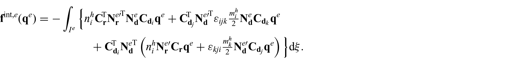
In order to simplify notation and to prevent possible clash of notation with Einstein summation convention we subsequently use the definitions ${\mathbf{N}}_{\mathbf{r}}:={\mathbf{N}}_{p_{\mathbf{r}}}$ , ${\mathbf{N}}_{\mathbf{d}}:={\mathbf{N}}_{p_{{\mathbf{d}}_i}}$ and ${\mathbf{N}}_{\lambda }:={\mathbf{N}}_{p_{\lambda }}$ . Inserting the discrete kinematic quantities into the internal virtual work (14), their corresponding discrete counterpart is given by

$$\delta W^{\mathrm{int},\mathrm{h}}=\delta {\mathbf{q}}^{\mathrm{T}}{\mathbf{f}}^{\mathrm{int}}(\mathbf{q}),{\mathbf{f}}^{\mathrm{int}}(\mathbf{q})={\sum }_{e=1}^n{{\mathbf{C}}^e}^{\mathrm{T}}{\mathbf{f}}^{\mathrm{int},e}({\mathbf{C}}^e\mathbf{q}),$$

with the internal forces of the element $e$ given by

$$\begin{array}{c}{\mathbf{f}}^{\mathrm{int},e}({\mathbf{q}}^e)=-{\int }_{I^e}\{n_i^h{\mathbf{C}}_{\mathbf{r}}^{\mathrm{T}}{{\mathbf{N}}_{\mathbf{r}}^{e\prime }}^{\mathrm{T}}{\mathbf{N}}_{\mathbf{d}}^e{\mathbf{C}}_{{\mathbf{d}}_i}{\mathbf{q}}^e+{\mathbf{C}}_{{\mathbf{d}}_j}^{\mathrm{T}}{{\mathbf{N}}_{\mathbf{d}}^{e\prime }}^{\mathrm{T}}{\epsilon }_{\mathrm{ijk}}\frac{m_i^h}{2}{\mathbf{N}}_{\mathbf{d}}^e{\mathbf{C}}_{{\mathbf{d}}_k}{\mathbf{q}}^e\hfill \\ \multicolumn{1}{c}{+{\mathbf{C}}_{{\mathbf{d}}_i}^{\mathrm{T}}{{\mathbf{N}}_{\mathbf{d}}^e}^{\mathrm{T}}(n_i^h{\mathbf{N}}_{\mathbf{r}}^{e\prime }{\mathbf{C}}_{\mathbf{r}}{\mathbf{q}}^e+{\epsilon }_{\mathrm{kji}}\frac{m_k^h}{2}{\mathbf{N}}_{\mathbf{d}}^{e\prime }{\mathbf{C}}_{{\mathbf{d}}_j}{\mathbf{q}}^e)\}\mathrm{d}\xi .}\end{array}$$

For the computation of the discretized generalized forces $n_i^h$ and $m_i^h$ the according strain measures

$${\mathrm{\Gamma }}_i^h=\frac{1}{J}{{\mathbf{q}}^e}^{\mathrm{T}}{\mathbf{C}}_{\mathbf{r}}^{\mathrm{T}}{\mathbf{N}}_{\mathbf{r}}^{\mathrm{T}}{\mathbf{N}}_{\mathbf{d}}^e{\mathbf{C}}_{{\mathbf{d}}_i}{\mathbf{q}}^e,{\mathrm{K}}_i^h=\frac{{\epsilon }_{\mathrm{ijk}}}{2J}{{\mathbf{q}}^e}^{\mathrm{T}}{\mathbf{C}}_{{\mathbf{d}}_k}^{\mathrm{T}}{\mathbf{N}}_{\mathbf{d}}^{\mathrm{T}}{\mathbf{N}}_{\mathbf{d}}^{e\prime }{\mathbf{C}}_{{\mathbf{d}}_j}{\mathbf{q}}^e$$

(34)

are required. As shown by [4] the discretized strain measures (34) still fulfill the objectivity requirement which is demonstrated numerically in Section 4.3.

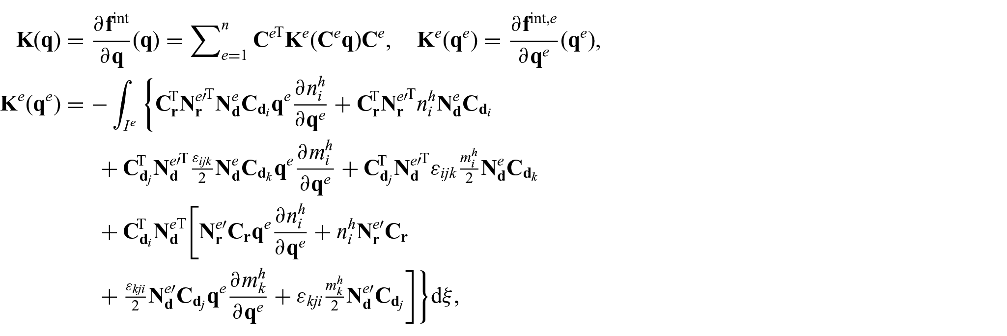
For convenience also the stiffness matrix, i.e., the partial derivative of the internal forces with respect to the generalized coordinates, is given

$$\begin{array}{c}\mathbf{K}(\mathbf{q})=\frac{\partial {\mathbf{f}}^{\mathrm{int}}}{\partial \mathbf{q}}(\mathbf{q})={\sum }_{e=1}^n{{\mathbf{C}}^e}^{\mathrm{T}}{\mathbf{K}}^e({\mathbf{C}}^e\mathbf{q}){\mathbf{C}}^e,{\mathbf{K}}^e({\mathbf{q}}^e)=\frac{\partial {\mathbf{f}}^{\mathrm{int},e}}{\partial {\mathbf{q}}^e}({\mathbf{q}}^e),\hfill \\ \multicolumn{1}{c}{{\mathbf{K}}^e({\mathbf{q}}^e)=-{\int }_{I^e}\{{\mathbf{C}}_{\mathbf{r}}^{\mathrm{T}}{{\mathbf{N}}_{\mathbf{r}}^{e\prime }}^{\mathrm{T}}{\mathbf{N}}_{\mathbf{d}}^e{\mathbf{C}}_{{\mathbf{d}}_i}{\mathbf{q}}^e\frac{\partial n_i^h}{\partial {\mathbf{q}}^e}+{\mathbf{C}}_{\mathbf{r}}^{\mathrm{T}}{{\mathbf{N}}_{\mathbf{r}}^{e\prime }}^{\mathrm{T}}{n}_i^h{\mathbf{N}}_{\mathbf{d}}^e{\mathbf{C}}_{{\mathbf{d}}_i}}\\ \multicolumn{1}{c}{+{\mathbf{C}}_{{\mathbf{d}}_j}^{\mathrm{T}}{{\mathbf{N}}_{\mathbf{d}}^{e\prime }}^{\mathrm{T}}\frac{{\epsilon }_{\mathrm{ijk}}}{2}{\mathbf{N}}_{\mathbf{d}}^e{\mathbf{C}}_{{\mathbf{d}}_k}{\mathbf{q}}^e\frac{\partial m_i^h}{\partial {\mathbf{q}}^e}+{\mathbf{C}}_{{\mathbf{d}}_j}^{\mathrm{T}}{{\mathbf{N}}_{\mathbf{d}}^{e\prime }}^{\mathrm{T}}{\epsilon }_{\mathrm{ijk}}\frac{m_i^h}{2}{\mathbf{N}}_{\mathbf{d}}^e{\mathbf{C}}_{{\mathbf{d}}_k}}\\ \multicolumn{1}{c}{+{\mathbf{C}}_{{\mathbf{d}}_i}^{\mathrm{T}}{{\mathbf{N}}_{\mathbf{d}}^e}^{\mathrm{T}}[{\mathbf{N}}_{\mathbf{r}}^{e\prime }{\mathbf{C}}_{\mathbf{r}}{\mathbf{q}}^e\frac{\partial n_i^h}{\partial {\mathbf{q}}^e}+n_i^h{\mathbf{N}}_{\mathbf{r}}^{e\prime }{\mathbf{C}}_{\mathbf{r}}}\\ \multicolumn{1}{c}{+\frac{{\epsilon }_{\mathrm{kji}}}{2}{\mathbf{N}}_{\mathbf{d}}^{e\prime }{\mathbf{C}}_{{\mathbf{d}}_j}{\mathbf{q}}^e\frac{\partial m_k^h}{\partial {\mathbf{q}}^e}+{\epsilon }_{\mathrm{kji}}\frac{m_k^h}{2}{\mathbf{N}}_{\mathbf{d}}^{e\prime }{\mathbf{C}}_{{\mathbf{d}}_j}]\}\mathrm{d}\xi ,}\end{array}$$

where the derivative of the discretized generalized internal forces are computed as

$$\frac{\partial n_i^h}{\partial {\mathbf{q}}^e}=\frac{\partial n_i}{\partial {\mathrm{\Gamma }}_j}\frac{\partial {\mathrm{\Gamma }}_j^h}{\partial {\mathbf{q}}^e}+\frac{\partial n_i}{\partial {\mathrm{K}}_j}\frac{\partial {\mathrm{K}}_j^h}{\partial {\mathbf{q}}^e},\frac{\partial m_i^h}{\partial {\mathbf{q}}^e}=\frac{\partial m_i}{\partial {\mathrm{\Gamma }}_j}\frac{\partial {\mathrm{\Gamma }}_j^h}{\partial {\mathbf{q}}^e}+\frac{\partial m_i}{\partial {\mathrm{K}}_j}\frac{\partial {\mathrm{K}}_j^h}{\partial {\mathbf{q}}^e}.$$

In the case of hyperelastic materials the derivatives of the contact forces and couples can be calculated from the strain energy function $W$ as follows

$$\frac{\partial n_i}{\partial {\mathrm{\Gamma }}_j}=\frac{{\partial }^{2}W}{\partial {\mathrm{\Gamma }}_i\partial {\mathrm{\Gamma }}_j},\frac{\partial n_i}{\partial {\mathrm{K}}_j}=\frac{{\partial }^{2}W}{\partial {\mathrm{\Gamma }}_i\partial {\mathrm{K}}_j},\frac{\partial m_i}{\partial {\mathrm{\Gamma }}_j}=\frac{{\partial }^{2}W}{\partial {\mathrm{K}}_i\partial {\mathrm{\Gamma }}_j},\frac{\partial m_i}{\partial {\mathrm{K}}_j}=\frac{{\partial }^{2}W}{\partial {\mathrm{K}}_i\partial {\mathrm{K}}_j}.$$

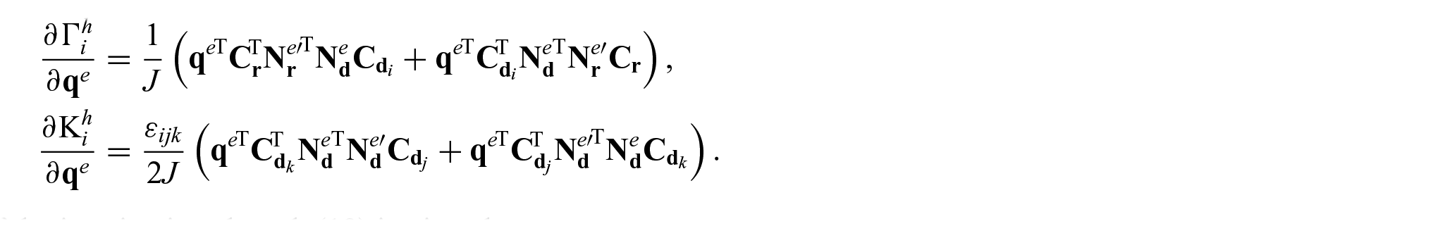
For the sake of completeness the derivatives of the discretized strain measures with respect to the generalized coordinates are also given

$$\begin{array}{c}\frac{\partial {\mathrm{\Gamma }}_i^h}{\partial {\mathbf{q}}^e}=\frac{1}{J}({{\mathbf{q}}^e}^{\mathrm{T}}{\mathbf{C}}_{\mathbf{r}}^{\mathrm{T}}{{\mathbf{N}}_{\mathbf{r}}^{e\prime }}^{\mathrm{T}}{\mathbf{N}}_{\mathbf{d}}^e{\mathbf{C}}_{{\mathbf{d}}_i}+{{\mathbf{q}}^e}^{\mathrm{T}}{\mathbf{C}}_{{\mathbf{d}}_i}^{\mathrm{T}}{{\mathbf{N}}_{\mathbf{d}}^e}^{\mathrm{T}}{\mathbf{N}}_{\mathbf{r}}^{e\prime }{\mathbf{C}}_{\mathbf{r}}),\hfill \\ \multicolumn{1}{c}{\frac{\partial {\mathrm{K}}_i^h}{\partial {\mathbf{q}}^e}=\frac{{\epsilon }_{\mathrm{ijk}}}{2J}({{\mathbf{q}}^e}^{\mathrm{T}}{\mathbf{C}}_{{\mathbf{d}}_k}^{\mathrm{T}}{{\mathbf{N}}_{\mathbf{d}}^e}^{\mathrm{T}}{\mathbf{N}}_{\mathbf{d}}^{e\prime }{\mathbf{C}}_{{\mathbf{d}}_j}+{{\mathbf{q}}^e}^{\mathrm{T}}{\mathbf{C}}_{{\mathbf{d}}_j}^{\mathrm{T}}{{\mathbf{N}}_{\mathbf{d}}^{e\prime }}^{\mathrm{T}}{\mathbf{N}}_{\mathbf{d}}^e{\mathbf{C}}_{{\mathbf{d}}_k}).}\end{array}$$

The discrete version of the inertia virtual work (18) is given by

$$\delta W^{\mathrm{dyn},\mathrm{h}}=-\delta {\mathbf{q}}^{\mathrm{T}}\mathbf{M}\stackrel{··}{\mathbf{q}},\mathbf{M}={\sum }_{e=1}^n{{\mathbf{C}}^e}^{\mathrm{T}}{\mathbf{M}}^e{\mathbf{C}}^e,$$

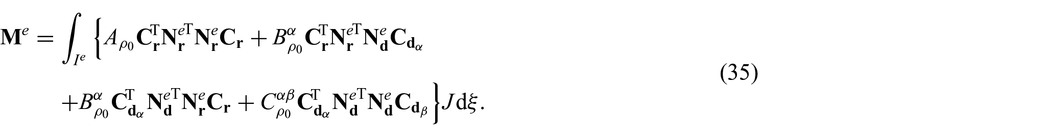
with the element mass matrix being defined as

$$\begin{array}{c}{\mathbf{M}}^e={\int }_{I^e}\{A_{{\rho }_0}{\mathbf{C}}_{\mathbf{r}}^{\mathrm{T}}{{\mathbf{N}}_{\mathbf{r}}^e}^{\mathrm{T}}{\mathbf{N}}_{\mathbf{r}}^e{\mathbf{C}}_{\mathbf{r}}+B_{{\rho }_0}^{\alpha }{\mathbf{C}}_{\mathbf{r}}^{\mathrm{T}}{{\mathbf{N}}_{\mathbf{r}}^e}^{\mathrm{T}}{\mathbf{N}}_{\mathbf{d}}^e{\mathbf{C}}_{{\mathbf{d}}_{\alpha }}\hfill \\ +B_{{\rho }_0}^{\alpha }{\mathbf{C}}_{{\mathbf{d}}_{\alpha }}^{\mathrm{T}}{{\mathbf{N}}_{\mathbf{d}}^e}^{\mathrm{T}}{\mathbf{N}}_{\mathbf{r}}^e{\mathbf{C}}_{\mathbf{r}}+C_{{\rho }_0}^{\alpha \beta }{\mathbf{C}}_{{\mathbf{d}}_{\alpha }}^{\mathrm{T}}{{\mathbf{N}}_{\mathbf{d}}^e}^{\mathrm{T}}{\mathbf{N}}_{\mathbf{d}}^e{\mathbf{C}}_{{\mathbf{d}}_{\beta }}\}J\mathrm{d}\xi .\hfill \end{array}$$

(35)

Note the element mass matrix is constant but singular with respect to the degrees of freedom of the first director, i.e., ${\mathbf{q}}_{{\mathbf{d}}_1}^e$ , which is of crucial importance for the design of an appropriate time integration scheme, see Section 4.5.

Without any pitfalls, the external virtual work (16) can be discretized in the same way as previously which yields a discrete external virtual work of the form

$$\delta W^{\mathrm{ext},\mathrm{h}}=\delta {\mathbf{q}}^{\mathrm{T}}{\mathbf{f}}^{\mathrm{ext}}(t,\mathbf{q}).$$

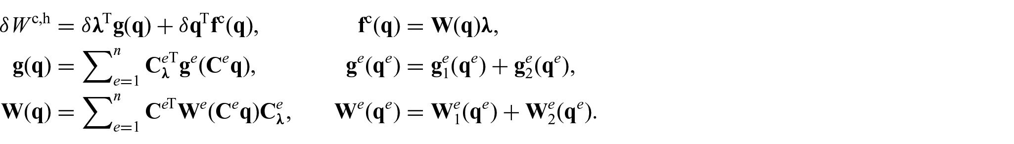
The spatial discretization can be completed by inserting the discretization of the Lagrange multipliers (32) and their variations (33) into the virtual work of the constraints (25). Therefore, the discrete virtual work of the constraints can be expressed in terms of the discrete constraint equations $\mathbf{g}$ , the constraint forces ${\mathbf{f}}^{\mathrm{c}}$ , and the generalized force directions $\mathbf{W}$ , i.e.,

$$\begin{array}{c}\delta W^{\mathrm{c},\mathrm{h}}=\delta {\mathbf{\lambda }}^{\mathrm{T}}\mathbf{g}(\mathbf{q})+\delta {\mathbf{q}}^{\mathrm{T}}{\mathbf{f}}^{\mathrm{c}}(\mathbf{q}),{\mathbf{f}}^{\mathrm{c}}(\mathbf{q})=\mathbf{W}(\mathbf{q})\mathbf{\lambda },\hfill \\ \multicolumn{1}{c}{\mathbf{g}(\mathbf{q})={\sum }_{e=1}^n{{\mathbf{C}}_{\mathbf{\lambda }}^e}^{\mathrm{T}}{\mathbf{g}}^e({\mathbf{C}}^e\mathbf{q}),{\mathbf{g}}^e({\mathbf{q}}^e)={\mathbf{g}}_1^e({\mathbf{q}}^e)+{\mathbf{g}}_2^e({\mathbf{q}}^e),}\\ \multicolumn{1}{c}{\mathbf{W}(\mathbf{q})={\sum }_{e=1}^n{{\mathbf{C}}^e}^{\mathrm{T}}{\mathbf{W}}^e({\mathbf{C}}^e\mathbf{q}){\mathbf{C}}_{\mathbf{\lambda }}^e,{\mathbf{W}}^e({\mathbf{q}}^e)={\mathbf{W}}_1^e({\mathbf{q}}^e)+{\mathbf{W}}_2^e({\mathbf{q}}^e).}\end{array}$$

The discrete element constraint equations ${\mathbf{g}}^e$ are split into a first one corresponding to the director orthonormality and a second one incorporating the non-shearability as well as the inextensiblity. These constraint equations are

$$\begin{array}{c}{\mathbf{g}}_1^e={\int }_{I^e}{\mathbf{C}}_{{\lambda }_{\mathrm{ij}}}^{\mathrm{T}}{{\mathbf{N}}_{\lambda }^e}^{\mathrm{T}}[{{\mathbf{q}}^e}^{\mathrm{T}}{\mathbf{C}}_{{\mathbf{d}}_i}^{\mathrm{T}}{{\mathbf{N}}_{\mathbf{d}}^e}^{\mathrm{T}}{\mathbf{N}}_{\mathbf{d}}^e{\mathbf{C}}_{{\mathbf{d}}_j}{\mathbf{q}}^e-{\delta }_{\mathrm{ij}}]\mathrm{d}\xi ,\hfill \\ \multicolumn{1}{c}{{\mathbf{g}}_2^e={\int }_{I^e}{\mathbf{C}}_{{\lambda }_i}^{\mathrm{T}}{{\mathbf{N}}_{\lambda }^e}^{\mathrm{T}}[{{\mathbf{q}}^e}^{\mathrm{T}}{\mathbf{C}}_{{\mathbf{d}}_i}^{\mathrm{T}}{{\mathbf{N}}_{\mathbf{d}}^e}^{\mathrm{T}}{\mathbf{N}}_{\mathbf{r}}^{e\prime }{\mathbf{C}}_{\mathbf{r}}{\mathbf{q}}^e-{\delta }_{1i}]\mathrm{d}\xi .}\end{array}$$

In the same way, the two element generalized force directions of the constraint forces are

$$\begin{array}{c}{\mathbf{W}}_1^e={\int }_{I^e}[{\mathbf{C}}_{{\mathbf{d}}_i}^{\mathrm{T}}{{\mathbf{N}}_{\mathbf{d}}^e}^{\mathrm{T}}{\mathbf{N}}_{\mathbf{d}}^e{\mathbf{C}}_{{\mathbf{d}}_j}{\mathbf{q}}^e+{\mathbf{C}}_{{\mathbf{d}}_j}^{\mathrm{T}}{{\mathbf{N}}_{\mathbf{d}}^e}^{\mathrm{T}}{\mathbf{N}}_{\mathbf{d}}^e{\mathbf{C}}_{{\mathbf{d}}_i}{\mathbf{q}}^e]{\mathbf{N}}_{\lambda }^e{\mathbf{C}}_{{\lambda }_{\mathrm{ij}}}\mathrm{d}\xi ,\hfill \\ \multicolumn{1}{c}{{\mathbf{W}}_2^e={\int }_{I^e}[{\mathbf{C}}_{\mathbf{r}}^{\mathrm{T}}{{\mathbf{N}}_{\mathbf{r}}^{e\prime }}^{\mathrm{T}}{\mathbf{N}}_{\mathbf{d}}^e{\mathbf{C}}_{{\mathbf{d}}_i}{\mathbf{q}}^e+{\mathbf{C}}_{{\mathbf{d}}_i}^{\mathrm{T}}{{\mathbf{N}}_{\mathbf{d}}^e}^{\mathrm{T}}{\mathbf{N}}_{\mathbf{r}}^{e\prime }{\mathbf{C}}_{\mathbf{r}}{\mathbf{q}}^e]{\mathbf{N}}_{\lambda }^e{\mathbf{C}}_{{\lambda }_i}\mathrm{d}\xi .}\end{array}$$

Inserting all the discrete virtual work contributions into the principle of virtual work and demanding the virtual work to vanish for all virtual displacements $\delta \mathbf{q}$ and $\delta \mathbf{\lambda }$ the semi-discrete equations of motion, which are still continuous in time, are obtained

$$\begin{array}{c}\mathbf{M}\stackrel{··}{\mathbf{q}}-{\mathbf{f}}^{\mathrm{int}}(\mathbf{q})-{\mathbf{f}}^{\mathrm{ext}}(t,\mathbf{q})-\mathbf{W}(\mathbf{q})\mathbf{\lambda }=0,\hfill \\ \multicolumn{1}{c}{\mathbf{g}(\mathbf{q})=0.}\end{array}$$

(36)

These equations of motion together with appropriate boundary and initial conditions can be discretized by a suitable time stepping scheme. By omitting the virtual work contributions of inertia effects and allowing the external forces to depend only on the generalized coordinates $\mathbf{q}$ , the discrete static equilibrium equations, i.e.,

$$\mathbf{R}(\mathbf{q},\mathbf{\lambda })=\left(\begin{array}{c}{\mathbf{f}}^{\mathrm{int}}(\mathbf{q})+{\mathbf{f}}^{\mathrm{ext}}(\mathbf{q})+\mathbf{W}(\mathbf{q})\mathbf{\lambda }\hfill \\ \multicolumn{1}{c}{\mathbf{g}(\mathbf{q})}\end{array}\right)$$

(37)

can be solved using a Newton–Raphson method for the case when no limit points are expected. Otherwise, the most simple way to overcome such points and for tracing the post-buckling paths a Riks-type algorithm [43] or the spherical arc-length method [44] can be used. A formulation of such an algorithm for constrained mechanical systems can be found in [45]. Applications to planar beam structures are found in [45–47].

4. Numerical examples

In this section, representative numerical problems are investigated. They are carefully selected in order to verify the correct derivation and implementation of the three presented beam models. The section starts with a validation of the numerical implemented beam models using analytical solutions and semi-analytic solutions found by elliptic integrals. Subsequently, an existing large deformation finite element simulation is reproduced. The section concludes with a dynamic real-world example demonstrating the practical benefit of the presented beam models. Throughout this section, the Timoshenko beam model is abbreviated by a $T$ , the Euler–Bernoulli beam by an $E$ and the inextensible Euler–Bernoulli beam by an $I$ .

Unless stated otherwise in the subsequent examples the beam centerline is discretized using B-spline shape functions of polynomial degree $p_{\mathbf{r}}=p$ . As indicated by the linearized theory in Section 2.8, it might be of advantage to discretize the directors using a B-spline corresponding to a polynomial of degree $p_{{\mathbf{d}}_i}=p_{\mathbf{r}}-1$ . Without mathematical proof, we use $p_{\lambda }=p_{{\mathbf{d}}_i}$ for the discretization of the Lagrange multipliers. Numerical investigations have pointed out that other possible values for discretizing the Lagrange multipliers, e.g. $p_{\lambda }=p_{\mathbf{r}}$ , lead to a singular iteration matrix of the used Newton–Raphson scheme.

4.1. Elliptic integrals solutions of Euler’s elastica

Let us consider an initially straight beam of length $L=2\pi$ with axial stiffness $E_1=5$ , shear stiffnesses $E_2=E_3=1$ , torsional stiffness $F_1=0.5$ and bending stiffnesses $F_2=F_3=2$ . The beam, which points in ${\mathbf{e}}_1$ -direction, is clamped at its left and subjected to a constant point force and couple at the other end. For the inextensible Euler–Bernoulli beam, this kind of problem is solved analytically by [48, Section 2.4] using the first and second elliptic integrals, defined as

$$F(\theta ,p)={\int }_0^{\theta }(1-p^2\stackrel{2}{\sin }\tilde{\theta }{)}^{-\frac{1}{2}}\mathrm{d}\tilde{\theta },E(\theta ,p)={\int }_0^{\theta }(1-p^2\stackrel{2}{\sin }\tilde{\theta }{)}^{\frac{1}{2}}\mathrm{d}\tilde{\theta },$$

see, for instance, [49] for a general introduction to elliptic integrals. Let the external point force $\mathbf{F}$ and couple $\mathbf{M}$ at the beam’s end $s=L$ solely depend on a force parameter ${\alpha }^2$ and read

$$\mathbf{F}=-P{\mathbf{e}}_2,\mathbf{M}=-M{\mathbf{e}}_3,P={\left(\frac{\alpha }{L}\right)}^2{F}_2,M=-2.5P.$$

The external moment $M$ , rotating clockwise with respect to the ${\mathbf{e}}_1$ – ${\mathbf{e}}_2$ -plane, can be replaced by a force $P$ with rigid lever $e=M/P$ . Further, by introducing a dimensionless parameter $k=\sqrt{P/F_2}$ the inextensibility condition relates the material point $s$ with the angle $\varphi (s)$ via

$$\mathrm{ks}=F(\varphi (s),p)-F({\varphi }_C,p),\cos {\varphi }_C=\mathrm{ek}/2p,$$

(38)

with the unknown constant $p$ . Further it can be shown that the angle at $s=L$ can be determined from $\sin \varphi (L)=\sin {\varphi }_B=1/(p\sqrt{2})$ . Thus, for given values of the external force $P$ , couple $M$ , and beam length $L$ , we can solve (38) for $p$ by a root-finding method, e.g., a bisection method. With the value of $p$ at hand we can again solve (38), but this time for the angle $\varphi$ at an arbitrary material point $s$ . The beam’s centerline $\mathbf{r}(s)=x(s){\mathbf{e}}_1+y(s){\mathbf{e}}_2$ can then be computed by the values of the horizontal and vertical deflections given by

$$\begin{array}{c}x(s)=2p[\cos ({\varphi }_B)-\cos (\varphi )]/k,\hfill \\ y(s)=-[2E({\varphi }_B,p)-2E(\varphi ,p)+F(\varphi ,p)-F({\varphi }_B,p)]/k.\hfill \end{array}$$

For the discretization of the used finite element models, $n=12$ cubic B-spline elements were used. The numerical solution was obtained by application of a load controlled Newton–Raphson method with 10 load steps and a convergence tolerance of ${10}^{-12}$ with respect to the maximum absolute error of the static residual (37) up to a maximal load factor of ${\alpha }^2=10$ .

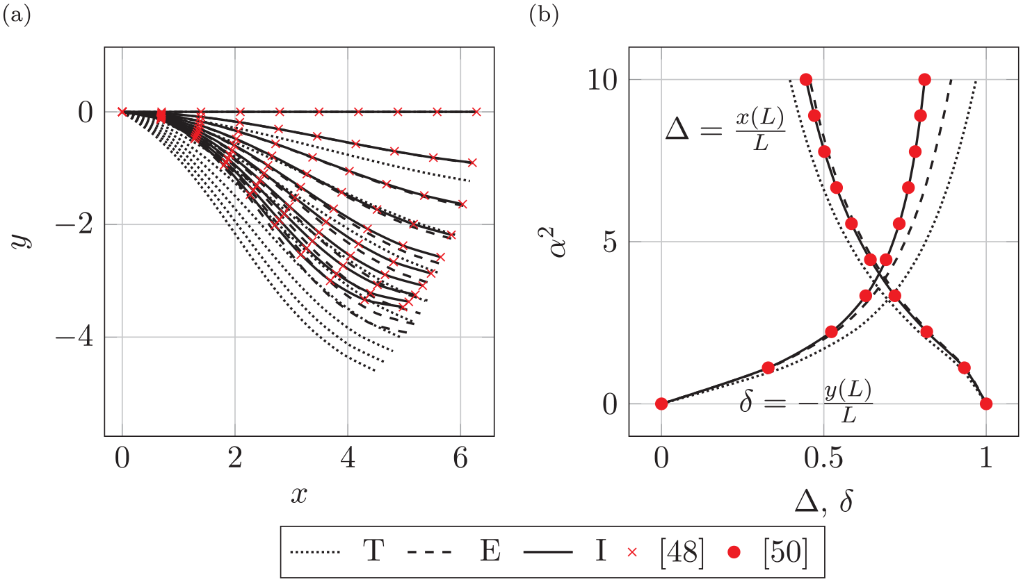
In Figure 3(a), the configurations for the different beam models are compared with the previous presented solution found by using elliptic integrals. For the inextensible Euler–Bernoulli beam model all configurations are in excellent accordance with the elliptic integral solution. The extensible Euler–Bernoulli beam model and the Timoshenko beam model yield larger overall deformations due to the allowed axial and shear deformations, respectively.

Figure 3.

(a) Deformed configurations and analytical solution given by [48]. (b) Dimensionless displacements versus dimensionless force for the case of no external couple; the inextensible solution coincides with the characteristic curves reported in [50].

For the case of vanishing external couple the analytic solution found in [50] and [48, Section 2.2] is obtained. In Figure 3(b), the normalized horizontal and vertical displacements given by $\delta =-y(L)/L$ and $\mathrm{\Delta }=x(L)/L$ are depicted for given load parameters ${\alpha }^2$ . It can be observed that again the inextensible Euler–Bernoulli beam model can reproduce the results obtained by using elliptic integrals. Accordingly, the Timoshenko and Euler–Bernoulli beam models lead to slightly different results, owing to their less-restricted kinematics.

This example demonstrates the power of the proposed constrained beam formulation. On the one hand, the complete kinematics of the Timoshenko beam can be represented and, on the other hand, additional beam models can be derived from it by simply adding further constraints. For the most constrained beam model, the inextensible Euler–Bernoulli beam, the solution found by elliptic integrals is exactly reproduced which can be seen as a numerical proof of the presented derivation and implementation.

4.2. 3D bending and twist

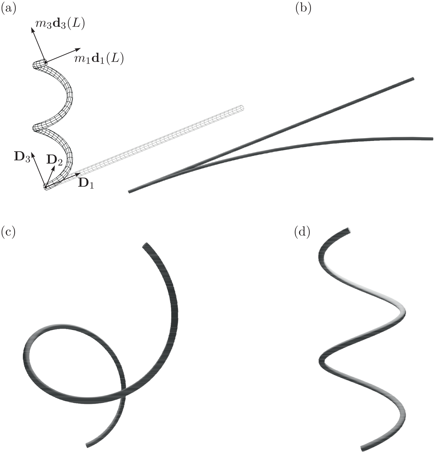
In this example an initially straight beam should be deformed to a perfect helix with $n=2$ coils of radius $R_0=10$ and height $h=50$ around the ${\mathbf{e}}_3$ -axis, see Figure 4(a).

Figure 4.

(a) Schematic sketch of the initial (gray) and deformed (black) configuration of the helix problem. 3D rendered configurations for $\zeta =100$ , $n=16$ elements and equal order shape functions: (b) $p_{\mathbf{r}}=p_{{\mathbf{d}}_i}=p_{\lambda }=p=1$ straight initial configuration and configuration with strong locking; (c) $p_{\mathbf{r}}=p_{{\mathbf{d}}_i}=p_{\lambda }=p=2$ configuration with intermediate locking; (d) $p_{\mathbf{r}}=p_{{\mathbf{d}}_i}=p_{\lambda }=3$ configuration without locking.

Introducing the abbreviation $c=h/(R_{0}2\pi n)$ such a deformed beam centerline can be described by

$${\mathbf{r}}^{*}(s)=R_0\sin \alpha (s){\mathbf{e}}_1-R_0\cos \alpha (s){\mathbf{e}}_2+c{R}_0\alpha (s){\mathbf{e}}_3,\alpha (s)=2\pi \mathrm{ns}/L.$$

(39)

Depending on the slenderness $\zeta$ , the beam has a circular cross section of diameter $d=L/\zeta$ , radius $r=d/2$ , area $A=\pi r^2$ , and the moments of area $I_2=I_3=\frac{\pi }{4}{r}^4$ and $I_1=\frac{\pi }{2}{r}^4$ . Using the Young’s and shear moduli $E=1$ and $G=0.5$ , respectively, and by assuming material properties given by $E_1=\mathrm{EA}$ , $E_2=E_3=\mathrm{GA}$ , $F_1=G{I}_1$ , and $F_{\alpha }=E{I}_{\alpha }$ , this yields $E_1=A$ , $E_2=E_3=A/2$ , and $F_1=F_2=F_3=\frac{\pi }{4}{r}^4$ . In order to find the force boundary conditions for this specific example, we apply a so called inverse procedure. ³ The tangent vector of the curve is

$${\mathbf{r}}^{*\prime }(s)=R_0\alpha \prime \cos \alpha (s){\mathbf{e}}_1+R_0\alpha \prime \sin (s){\mathbf{e}}_2+c{R}_0\alpha \prime {\mathbf{e}}_3.$$

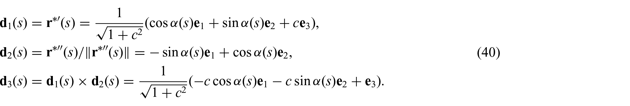
If the beam should not be elongated during the deformation, its tangent vectors Euclidean norm has to be unity, i.e., $\parallel {\mathbf{r}}^{*\prime }(s)\parallel =1$ , from which the total beam length $L=\sqrt{1+c^2}{R}_{0}2\pi n$ can be deduced. Further, the Frenet–Serret frame of the deformed curve is given by the directors

$$\begin{array}{cc}{\mathbf{d}}_1(s)\hfill & ={\mathbf{r}}^{*\prime }(s)=\frac{1}{\sqrt{1+c^2}}(\cos \alpha (s){\mathbf{e}}_1+\sin \alpha (s){\mathbf{e}}_2+c{\mathbf{e}}_3),\hfill \\ \multicolumn{1}{c}{{\mathbf{d}}_2(s)}& ={\mathbf{r}}^{*″}(s)/\parallel {\mathbf{r}}^{*″}(s)\parallel =-\sin \alpha (s){\mathbf{e}}_1+\cos \alpha (s){\mathbf{e}}_2,\hfill \\ \multicolumn{1}{c}{{\mathbf{d}}_3(s)}& ={\mathbf{d}}_1(s)\times {\mathbf{d}}_2(s)=\frac{1}{\sqrt{1+c^2}}(-c\cos \alpha (s){\mathbf{e}}_1-c\sin \alpha (s){\mathbf{e}}_2+{\mathbf{e}}_3).\hfill \end{array}$$

(40)

Using $(1+c^2{)}^{-\frac{1}{2}}=R_{0}2\pi n/L=R_0\alpha \prime$ together with the derivatives of (40), the beam’s strain measures defined in (9) and (11) can be computed straightforwardly and lead to

$${\mathrm{\Gamma }}_1=1,{\mathrm{\Gamma }}_2={\mathrm{\Gamma }}_3=0,{\mathrm{K}}_1=c{R}_0\alpha {\prime }^2,{\mathrm{K}}_2=0,{\mathrm{K}}_3=R_0\alpha {\prime }^2.$$

From the strain energy density function (15), we can evaluate the constitutive relations (12) yielding the constant components of the contact forces and contact couples

$$n_i=0,m_1=F_1{\mathrm{K}}_1,m_2=0,m_3=F_3{\mathrm{K}}_3.$$

(41)

If we solely allow external forces and couples at the two end points of the beam but no distributed ones, by inserting (41) into the differential equation of the nonlinear Timoshenko beam, see [1], we obtain the requirement that $F_1=F_3$ . This condition is satisfied for the given problem setup. Thus, the desired deformation is obtained by application of the constant moment in the body fixed frame of the beam’s end point given by

$$\mathbf{m}=m_1{\mathbf{d}}_1(L)+m_3{\mathbf{d}}_3(L).$$

For a numerical simulation, the beam has to be clamped at $\mathbf{r}(0)=-R_0{\mathbf{e}}_2$ with an orientation given by the director frame ${\mathbf{d}}_1(0)=R_0\alpha \prime ({\mathbf{e}}_1+c{\mathbf{e}}_3)$ , ${\mathbf{d}}_2(0)={\mathbf{e}}_2$ and ${\mathbf{d}}_3(0)=R_0\alpha \prime (-c{\mathbf{e}}_1+{\mathbf{e}}_3)$ . For the case of $h=0$ , the standard benchmark, i.e., bending to a perfect double circle in the ${\mathbf{e}}_1$ – ${\mathbf{e}}_2$ -plane, is obtained, cf. [32].

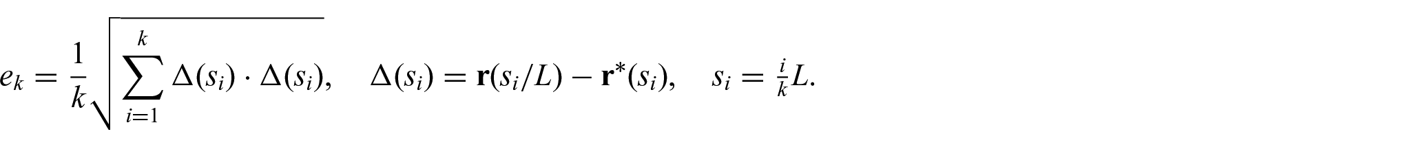
Subsequently, the numerically computed centerlines are compared with the analytical solution by means of the error

$$e_k=\frac{1}{k}\sqrt{{\sum }_{i=1}^k\mathrm{\Delta }(s_i)·\mathrm{\Delta }(s_i)},\mathrm{\Delta }(s_i)=\mathbf{r}(s_i/L)-{\mathbf{r}}^{*}(s_i),s_i=\frac{i}{k}L.$$

Again a force controlled Newton–Raphson method was performed using a convergence tolerance of ${10}^{-10}$ with respect to the maximum absolute error of the static residual (37). In a first step, using the slenderness ratio $\zeta =10$ , all presented beam formulations were evaluated for different polynomial degrees $p\in \{1,2,3,5\}$ and different numbers of elements $n\in \{16,32,64,128\}$ in order to study the convergence of the proposed formulations depending on the chosen polynomial degree. For comparative purpose, we computed this example with the director beam formulation presented in [4]. As indicated by the authors, a one-point quadrature rule has to be used in order to circumvent the strong locking phenomenon (even for moderate slenderness ratios). But even for a large number of elements and a low slenderness ratio $\zeta =10$ this problem could not be solved with the nodal enforcement of the constraints proposed by [4]. In Figure 5, the convergence behavior of the presented beam models is given. Owing to the pure bending deformation, independent of the chosen discretization, all three beam models led to the almost same errors. Discretizing all fields by the very same polynomial degree $p$ , the slope of convergence increases in contrast to discretizing the directors and Lagrange multipliers by polynomials of one degree lower than that of the centerline. This can easy be explained by the subsequent argument. The curvature terms (11) solely depend on the directors and their derivatives. Thus, shape functions of equal polynomial degree approximate the curvatures more accurately.

Figure 5.

Error $e_{100}$ versus the number of used elements $n$ with respect to the analytical solution of a perfect helix given in (39) for the Timoshenko , Euler–Bernoulli , and inextensible Euler–Bernoulli , beam using a constant slenderness ratio $\zeta =10$ and various polynomial degrees $p\in \{1,2,3,5\}$ with (a) $p_{\mathbf{r}}=p$ , $p_{{\mathbf{d}}_i}=p_{\lambda }=p-1$ and (b) $p_{\mathbf{r}}=p_{{\mathbf{d}}_i}=p_{\lambda }=p$ .

In a second example, the possible presence of locking, as presumed by the linear theory, is investigated. Using the same polynomial degree for all fields, i.e., $p_{\mathbf{r}}=p_{{\mathbf{d}}_i}=p_{\lambda }=p$ , for slenderness ratio $\zeta =100$ , and $n=16$ elements, the helix example was computed. While for $p=1$ and $p=2$ extreme locking occurs, $p=3$ could solve the problem, see Figure 4. However, a successful convergence of the Newton–Raphson scheme is very sensitive concerning the choice of the number of iteration steps. For slenderness ratio $\zeta =1000$ the problem could not be solved at all.

In a last example, all three beam models are computed with a polynomial degree $p_{\mathbf{r}}=p=3$ , $p_{{\mathbf{d}}_i}=p_{\lambda }=p-1=2$ , different numbers of elements $n\in \{16,32,64,128\}$ , and three slenderness ratios $\zeta \in \{10,100,1000\}$ . As can be observed in Figure 6, the error increases for higher slenderness ratios compared with that obtained for a moderate slenderness ratio. For increasing number of elements, the error converges to the one of the moderate slenderness. Thus, by using different order shape functions for the centerline $\mathbf{r}$ and the directors ${\mathbf{d}}_i$ , as indicated by the linear theory, the locking phenomenon is almost completely avoided at the cost of a poorer approximation of the curvature terms. Even an extreme slenderness ratio $\zeta =1000$ could be reliably solved.

Figure 6.

Error $e_{100}$ versus the number of used elements $n$ with respect to the analytical solution of a perfect helix given in (39) for the Timoshenko , Euler–Bernoulli , and inextensible Euler–Bernoulli , beam using a constant polynomial degree $p_{\mathbf{r}}=p=3$ , $p_{{\mathbf{d}}_i}=p_{\lambda }=p-1$ and different slenderness ratios $\zeta \in \{10,100,1000\}$ .

4.3. Numerical verification of objectivity

The next example, inspired by [51], is intended to serve several purposes. On the one hand, another analytical solution, i.e., pure bending to a perfect circle, a special case of the previously presented helix example, is investigated. On the other hand, the objectivity of the presented beam models can be verified through subsequently application of superimposed rigid-body rotations. These two cases are divided into four phases.

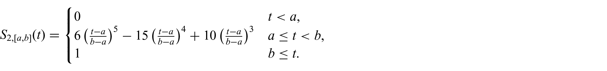
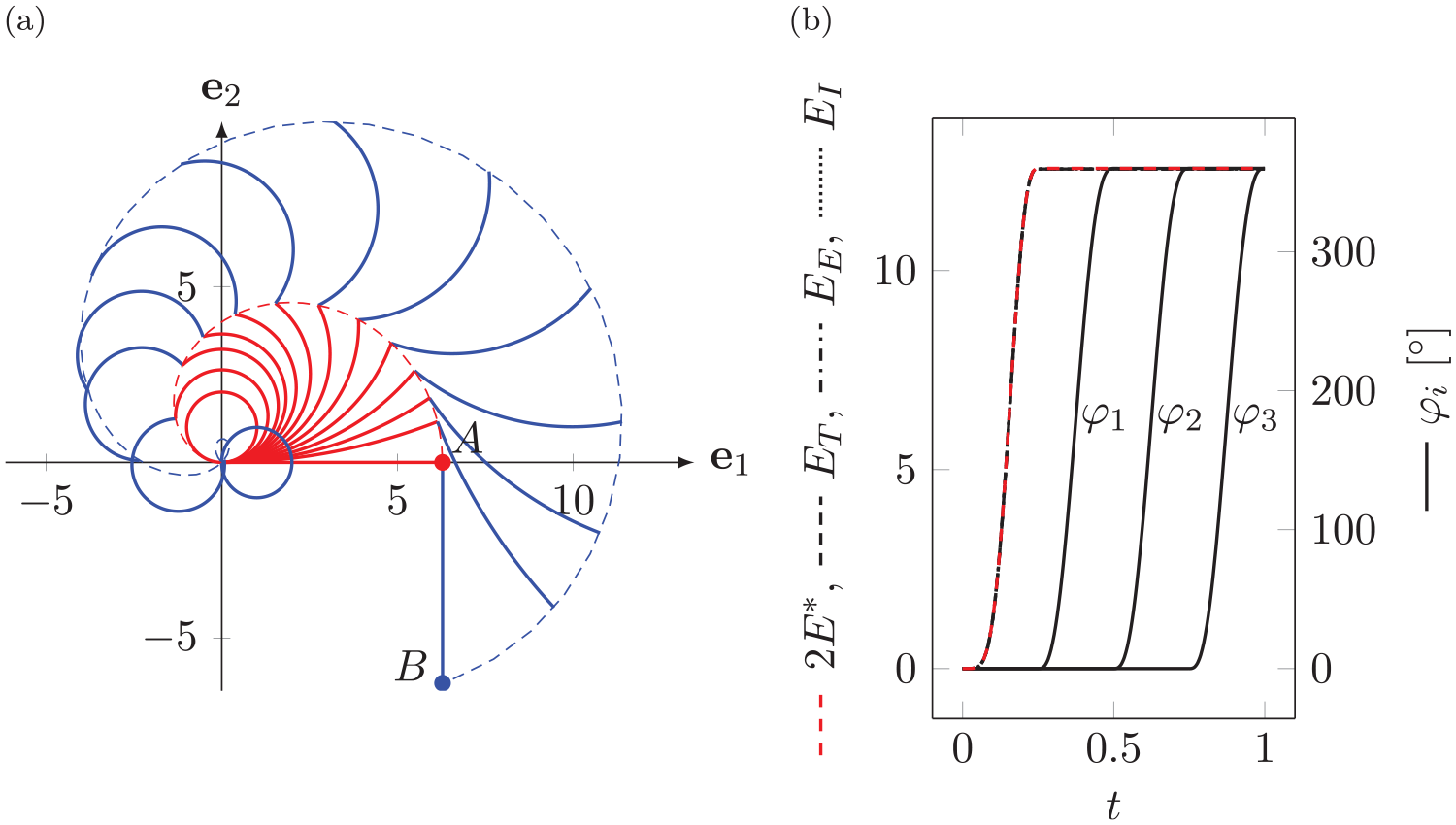
In the first phase two beams with the very same geometrical and material properties as used in the first example are initially placed in the ${\mathbf{e}}_1$ – ${\mathbf{e}}_2$ -plane forming an $L$ -shape, see Figure 7(a). The first beam, initially clamped at the origin, points in positive ${\mathbf{e}}_1$ direction. At its end, rotated by $-{90}^{°}$ around the ${\mathbf{e}}_3$ -axis, the second beam is attached pointing in negative ${\mathbf{e}}_2$ -direction, see Figure 7(a). For $t\in I_1=[0,0.25]$ an external couple $\mathbf{M}(t)=M(t){\mathbf{e}}_3$ is applied to the free end of the second beam. The external couple $M(t)=\frac{2\pi F_3}{L}{S}_{2,I_1}(t)$ depends on the second smooth step function $S_{2,I_1}$ on the interval $I_1$ defined as

$$S_{2,[a,b]}(t)=(\begin{array}{cc}0\hfill & t<a,\hfill \\ \multicolumn{1}{c}{6{\left(\frac{t-a}{b-a}\right)}^5-15{\left(\frac{t-a}{b-a}\right)}^4+10{\left(\frac{t-a}{b-a}\right)}^3}& a\le t<b,\hfill \\ \multicolumn{1}{c}{1}& b\le t.\hfill \end{array}$$

Figure 7.

(a) Deformed configurations starting from an undeformed $L$ -shape and ending with two perfect circles; beam end points trajectories given in (42). (b) Rotation angles and deformation energy for the Timoshenko ( $E_T$ ), Euler–Bernoulli ( $E_E$ ), and inextensible Euler–Bernoulli beam ( $E_I$ ) compared with analytically expected deformation energy.

This applied couple results in a deformed configuration of two perfect circles (see Figure 7(a)) and can be verified with similar arguments as in the previous example. By introducing the auxiliary functions

$$\mathrm{\Delta }(t)=\sin (\alpha (t))\frac{F_3}{M(t)},\delta (t)=[1-\cos (\alpha (t))]\frac{F_3}{M(t)},\alpha (t)=\frac{M(t)L}{F_3},$$

the trajectory of both beams’ end points can be computed as

$$\begin{array}{c}{\mathbf{P}}_A(t)=\mathrm{\Delta }(t){\mathbf{e}}_1+\delta (t){\mathbf{e}}_2,\hfill \\ \multicolumn{1}{c}{{\mathbf{P}}_B(t)={\mathbf{P}}_A(t)+[\cos (\alpha (t))\mathrm{\Delta }(t)-\sin (\alpha (t))\delta (t)]{\mathbf{e}}_1}\\ \multicolumn{1}{c}{+[\sin (\alpha (t))\mathrm{\Delta }(t)+\cos (\alpha (t))\delta (t)]{\mathbf{e}}_2.}\end{array}$$

(42)

As this loading case leads to a homogeneous bending deformation, we can identify the curvature in the beam to be ${\kappa }_3(t)=M(t)/F_3$ , all other strain measures are vanishing. By substituting the remaining stain measure into the total beams energy density (15) and integrating over the total beam length, we obtain the internal energy of a single beam given by

$$E^{*}(t)=\pi F_3{S}_{2,I_1}^2(t).$$

(43)

The systems total deformation energy is twice the value computed from (43). If the discretized strain measures (34) are objective, the systems total energy should remain constant in the phases $2$ – $4$ with the value (43). Then, in the subsequent three phases $I_2=[0.25,0.5]$ , $I_3=[0.5,0.75]$ , and $I_4=[0.75,1.0]$ , the clamping condition at the origin is replaced by successively applied rigid body rotations with the angles ${\phi }_i(t)=2\pi S_{2,I_i}$ , $i=1,2,3$ , around the respective axis of the inertial frame ${\mathbf{e}}_1$ , ${\mathbf{e}}_2$ , and ${\mathbf{e}}_3$ .

In Figure 7(a) it can be seen that the presented beam models are in perfect accordance with the analytically expected deformations and cannot be distinguished from each other owing to the pure bending deformation. In addition, the expected strain energy is obtained during the deformation, see Figure 7(b). After the first phase no loss or gain in strain energy is recognized. Thus, numerically all three presented beam models are in fact objective.

4.4. Beam patches with slope discontinuity

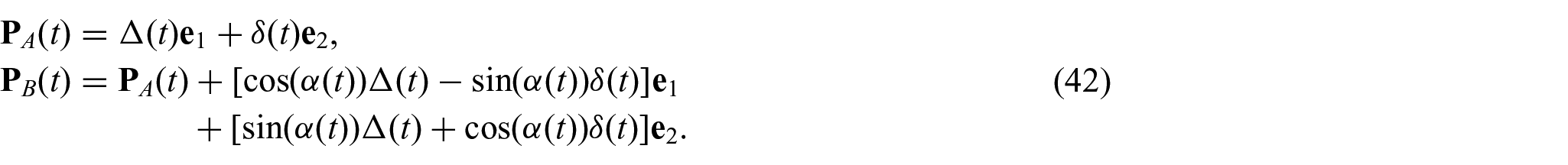
In this example a three-dimensional structure with two kinks (see Figure 8(a)) is subjected to a constant external force given by $\mathbf{F}=-F{\mathbf{e}}_1-F{\mathbf{e}}_3$ and magnitude $F=10$ . The structure consists of three initially straight beams of length $L=1$ , quadratic cross section with edge length $a=0.1$ , area $A=0.01$ , and the moments of area $I_1=a^4/6$ and $I_2=I_3=a^4/12$ . The first beam is clamped at the origin and points in positive ${\mathbf{e}}_1$ -direction. The second one pointing in the positive ${\mathbf{e}}_2$ -direction starts at the end of beam one. The third one starting from the end of beam two points in positive ${\mathbf{e}}_3$ -direction. The respective beams are connected to each other at right angles using six bilateral constraints, three for the connection of their centerlines and three for merging their cross-sectional orientations. In contrast to the previous examples, the hyperelastic material defined by the quadratic strain energy density mentioned in the note in Section 2.4 was used in order to obtain results that can be compared with finite element solutions found in the literature [28, 52]. Using the Young’s and shear moduli $E={10}^6$ and $G=E/2$ , respectively, and by assuming material properties given by $E_1=\mathrm{EA}$ , $E_2=E_3=\mathrm{GA}$ , $F_1=G{I}_1$ , and $F_{\alpha }=E{I}_{\alpha }$ , this yields $E_1=\mathrm{EA}$ , $E_2=E_3=E{a}^2/2$ , and $F_1=F_2=F_3=E{a}^4/12$ . We discretized each beam of the structure with $12$ cubic uniformly distributed elements. The problem was solved using $40$ iterations of a force controlled Newton–Raphson method with a convergence tolerance of ${10}^{-10}$ with respect to the maximum absolute error of the static residual (37).

Figure 8.

(a) Initial and final deformed configuration. (b) Beam tip deflection of the point of applied load and comparison with reference solution [28, 52].

In Figure 8(a) the reference and the final large deformed configuration of the three-dimensional structure can be seen. In Figure 8(b) the displacements of the point of applied load obtained by the presented beam models are compared with those reported in [28, 52].

For the given material properties all three beam models yield the identical results, which stems from the fact that the shear and axial stiffnesses are very high compared with the torsional and bending stiffnesses. Thus, the less-constrained beam models enforce the inextensiblity and non-shearability in the sense of a penalty method. Further, it can be noted that the deflection curves of the proposed beam models are in excellent agreement with the results reported in the literature.

4.5. Wilberforce pendulum

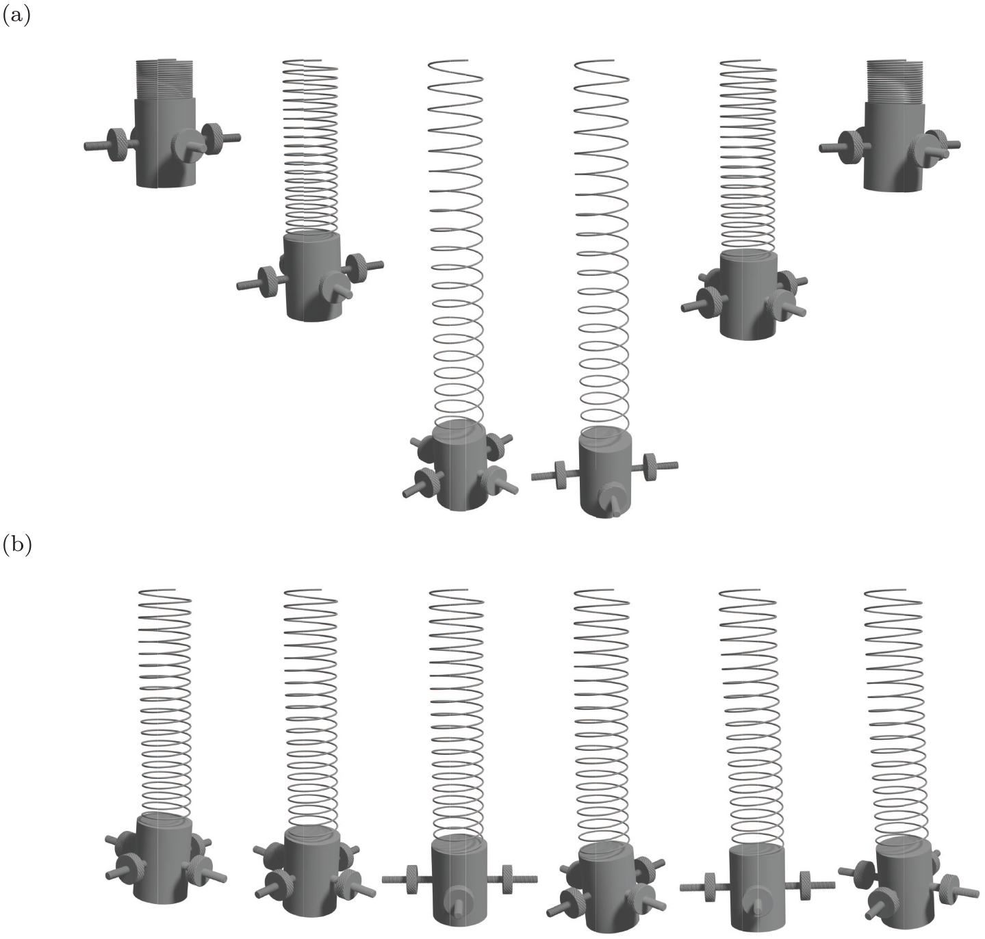
For demonstrating the proposed beam model’s strengths in dynamics and showing a predeformed initial configuration, the fascinating pendulum named after its inventor Lionel Robert Wilberforce was chosen. More than 100 years ago, Wilberforce presented investigations On the Vibrations of a Loaded Spiral Spring [53] which is clamped at its upper side. On the other side, perpendicular to the spring axis, a steel cylinder is attached. Four screws with adjustable nuts are symmetrically attached around the cylinder in order to change its moment of inertia, see Figure 9. When the cylinder is displaced vertically subjected to gravitational forces, it starts oscillating up and down. Owing to the coupling of bending and torsion of the deformed spring an additional torsional oscillation of the cylinder is induced. For properly adjusted moment of inertia of the cylinder, the vertical and torsional oscillation have a phase shift of $\pi /2$ , i.e., the maximal amplitude of the vertical oscillation coincides with a zero torsional amplitude and vice versa. There can be found several simplified analytical discussions of the Wilberforce pendulum in the literature [54–56].

Figure 9.

Configurations of the Wilberforce pendulum: (a) pure vertical oscillation and (b) pure torsional oscillation. The rendered animations are built using an open-source visualization tool [60].

Subsequently, the detailed mechanical model and its discretization is presented. The pendulum bob is modeled as a spatial rigid body of mass $m=0.469\mathrm{kg}$ and moment of inertia in the body fixed frame given by a diagonal matrix with entries ${\Theta }_{00}={\Theta }_{11}=0.0001468\mathrm{kg}{\mathrm{m}}^2$ and ${\Theta }_{22}=0.0001247\mathrm{kg}{\mathrm{m}}^2$ . It is parametrized using the Cardan angles $z$ – $x$ – $y$ . The spring, made of spring steel EN 10270-1 with density $\rho =7850\mathrm{kg}/{\mathrm{m}}^3$ , Young’s modulus $E=206\times {10}^9\mathrm{N}/{\mathrm{m}}^2$ , and shear modulus $G=81.5\times {10}^9\mathrm{N}/{\mathrm{m}}^2$ , has the undeformed shape of a perfect helix with $n=20$ coils, coil radius $R=16\mathrm{mm}$ , wire diameter $d=1\mathrm{mm}$ , and unloaded pitch $c=1\mathrm{mm}$ , i.e., the spring is in its block length. It is discretized by the presented Timoshenko beam model using $128$ cubic uniformly distributed elements. As no locking is expected for this kind of slenderness, we use the same shape functions for all fields, i.e., $p_{\mathbf{r}}=p_{{\mathbf{d}}_i}=p_{{\lambda }_k}=3$ in order to obtain a better approximation of the curvature terms.

Though a helix can be represented exactly by combining trigonometric functions and polynomials, i.e.,

$${\mathbf{r}}^{*}(\xi )=R\cos \varphi (\xi ){\mathbf{e}}_1+R\sin \varphi (\xi ){\mathbf{e}}_2+c\xi {\mathbf{e}}_3,\varphi (\xi )=2\pi n\xi ,$$

there is no exact representation for it by means of polynomials or rational polynomials. Thus, in order to obtain a helicoidal beam reference configuration, a fitting procedure has to be applied. This is done by minimizing the quadratic error of the beam centerline

$$e_k={\sum }_{i=1}^k\parallel \mathbf{r}({\xi }_i)-{\mathbf{r}}^{*}({\xi }_i){\parallel }^2.$$

An in-depth discussion of such a minimization procedure, where in addition a given number of points is exactly interpolated, e.g., the start and end points, is given in [39, Section 9.4.2]. For fitting the beams orientations, the very same procedure can be used by replacing the difference of the beam centerline with the difference of each director ${\mathbf{d}}_i$ and its corresponding vector of the helix space curve’s Frenet–Serret frame.

For the time integration of the semi-discrete equations of motion (36), a generalized- $\alpha$ scheme for constrained mechanical systems of index 3 is used, similar to that proposed by [57]. As mentioned in Section 3.2 the element mass matrix (35) is singular with respect to the generalized coordinates of the first director. Thus, the set of generalized coordinates has to be subdivided into purely algebraic ones ${\mathbf{q}}^{\mathrm{alg}}$ , i.e., those which have a singular mass matrix, and dynamical ones ${\mathbf{q}}^{\mathrm{dyn}}$ without that restriction. Owing to the special form of the used generalized- $\alpha$ method the internal iteration matrix does not get singular, even with a singular mass matrix, which is not guaranteed by an iterative time integration scheme. Thus, the only difference from the scheme proposed in [57] is that special care is necessary while computing consistent initial accelerations. We have to ensure that only those parts of the mass matrix corresponding to the dynamic generalized coordinates are inverted. All other initial accelerations have to be set zero. Further, we only use the right preconditioner matrix [57, Equation (10)]. An in-depth discussion about an optimal preconditioning of index 3 DAE solver is given in [58].

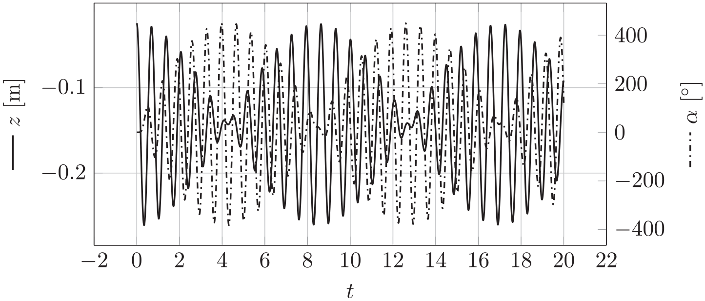
In Figure 9(a) and (b) snapshots of a pure vertical and torsional oscillation period can be seen and [59] shows a rendered video of the total integration time. For an integration time $T=20\mathrm{s}$ , a time step $\mathrm{\Delta }t=5\times {10}^{-4}\mathrm{s}$ , and the spectral radius at infinity ${\rho }_{\infty }=0.5$ , the eccentricity of the adjustable nuts was optimized leading to the given values for the moment of inertia in order to achieve an almost perfect phase shift, see Figure 10. Further it can be noted that the locking phenomenon previously discussed in Section 4.2 and the associated convergence problems are not present in such a real-world application, although the helicoidal spring is modeled by a slender beam. All three presented beam models were able to solve this problem yielding the same results owing to the high axial and shear stiffnesses.

Figure 10.

Vertical deflection and first Cardan angle of the pendulum bob. An almost perfect phase shift of vertical and torsional oscillation can be observed.

5. Conclusion

As a natural extension of existing finite element formulations of constraint beam models [4, 5, 28], the presented approach enforces the orthonormality constraints of the cross-sectional frame in a weak sense. This not only improves the convergence rate with respect to a finer discretization, but also enables the modeling of three kinematically different beam models within a single theory. Depending on the number of additionally chosen constraints, a spatial precurved nonlinear Timoshenko, Euler–Bernoulli, or inextensible Euler–Bernoulli beam model is obtained. Owing to the used intrinsic beam theory, arbitrary constitutive relations can be modeled by choosing an appropriate strain energy function, solely depending on the presented objective strain measures.

Exploiting a direct interpolation of the cross-sectional director frame, the present formulation avoids the difficulties of interpolating rotations arising in the minimal formulation of a spatial Timoshenko beam model [20, 21]. Further, it should be noted that it retains the property of objectivity during discretization. However, it has its own disadvantages. Instead of ordinary differential equations, a set of index 3 differential algebraic equations is obtained after spatial discretization. This requires the usage of advanced time integration schemes, e.g., the generalized- $\alpha$ solver for index 3 DAEs presented in [57].

For the most-constrained beam formulation, analytical solutions by means of elliptic integrals can be reproduced. This numerically proves its correct derivation and implementation. Further, homogeneous pure bending deformations can be reproduced by all presented beam models which validates the correctness of torsion and flexure. In addition, existing finite element simulations as well as difficult dynamical behavior of real-world applications can be reproduced.

In order to almost completely avoid the locking phenomena appearing for increasingly thinner beams, the two kinematic fields (centerline $\mathbf{r}$ and directors ${\mathbf{d}}_i$ ) are discretized with B-spline shape functions of different, but tailored polynomial degrees. If this is not the case or when linear shape functions should be used for both kinematic fields, convergence problems arise as structures become increasingly thinner and locking occurs. This behavior of spatial Timoshenko beams is well known in the literature and makes them on a par with existing minimal formulations. There are different possibilities found in the literature to overcome these difficulties. On the one hand minimal formulated spatial Euler–Bernoulli beam models [9–12] or different constrained Euler–Bernoulli beam theories that explicitly ensure the vanishing shear deformations [61, 62] can be used. On the other hand, so-called intrinsically locking-free Timoshenko beam formulations [38, 63] have to be extended from the planar case to the spatial one. Another promising solution are so-called mixed formulations that introduce the internal forces and couples as independent variables in combination with isogeometric collocation methods [25].

Future research should include the application of spatial beam finite element models to real-time control applications in soft robotics [64–66]. Further, the constrained numerical beam models have to be validated using existing experimental data [67]. Finally, investigations of the planar case as the analysis of bifurcations and tracing the post-buckling path of beam structures [68], the modal analysis of Timoshenko beams [69] as well as a special class of metamaterials, so-called panthographic materials, see among others [70–74], should be investigated by using spatial constrained beam theories.