Variational principles of nonlinear magnetoelastostatics and their correspondences

Abstract

We derive the equations of nonlinear magnetoelastostatics using several variational formulations involving the mechanical deformation and an independent field representing the magnetic component. An equivalence is also discussed, modulo certain boundary integrals or constant integrals, between these formulations using the Legendre transform and properties of Maxwell’s equations. Bifurcation equations based on the second variation are stated for the incremental fields as well for all five variational principles. When the total potential energy is defined over the infinite space surrounding the body, we find that the inclusion of certain terms in the energy principle, associated with the externally applied magnetic field, leads to slight changes in the Maxwell stress tensor and associated boundary conditions. Conversely, when the energy contained in the magnetic field is restricted to finite volumes, we find that there is a correspondence between the discussed formulations and associated expressions of physical entities. In view of a diverse set of boundary data and the nature of externally applied controls in the problems studied in the literature, along with an equally diverse list of variational principles employed in modelling, our analysis emphasises care in the choice of variational principle and unknown fields so that consistency with other choices is also satisfied.

1. Introduction

Magnetoelastostatics concerns the analysis of suitable phenomenological models for a physical description of the equilibrium in a certain type of deformable solid associated with multifunctional processes involving magnetic and elastic effects. The main property characterising these solids is the coupling between elastic deformation and magnetisation that they experience in the presence of externally applied mechanical and magnetic force fields [1–4]. The so-called magnetoelastic coupling is known to occur in response to a phenomenon involving reconfigurations of small magnetic domains while a continuum vector field is borne out of an averaging of microscopic and distributed subfields [5, 6]. Thus, an imposition of the magnetic field also induces a deformation of the material specimen in addition to the magnetic effects caused by the traditional mechanical forces [7].

With a history of more than five decades [8–14], the mathematical modelling of magnetoelasticity continues to be a vibrant area of research. The presence of strong magnetoelastic coupling in some manufactured materials, such as magnetorheological elastomers (MREs) [1], allows the subject to be relevant for a large number of potential engineering and technological applications. Magnetorheological elastomers are composites made of ferromagnetic particles embedded in a polymer matrix. Magnetisation of the ferromagnetic domains in the presence of an external magnetic field, and the resulting interactions, leads to a change in macroscopically observable mechanical properties. As a result, MREs find applications in microrobotics [15, 16], sensors and actuators [17, 18], active vibration control [19], and waveguides [20, 21]. Constitutive modelling of MREs has been undertaken by appropriately considering the micromechanics and derivation of coupled field equations using homogenisation [5, 22], consideration of energy dissipation as a result of the viscoelasticity of the underlying matrix [23–26] and consideration of anisotropy as a result of ferromagnetic particle alignment [4, 27, 28].

The derivation of a consistent set of partial differential equations and boundary conditions that describe equilibrium, the analysis of the stability of equilibrium and the solution of the relevant partial differential equations via numerical techniques, such as the finite-element method, require development of appropriate variational principles. In this paper, we shall be concerned with the variational principles that have been postulated for the materials under the magnetoelastostatics assumptions and ignore any dynamic or dissipative effects. Current variational principles of magnetoelastostatics typically fall into two classes: principles based on the magnetic field or the magnetic induction as independent variables [29, 30] and principles based on a variant of the magnetisation as an independent variable [13, 31]. The typical starting point, definition of the total potential energy, is different in all these cases, while it results in certain correspondence between the Euler–Lagrange equations derived.

The twofold motivation of this paper is the study of equations for the statics problem as well as of the counterparts of bifurcation equations within the several variational formulations. Within the magnetisation-based principles, we discuss three different formulations that utilise, respectively, magnetisation field per unit volume, magnetisation per unit mass and another adaptation of magnetisation field as an independent entity. In fact, one of these variational principles analysed in this paper was postulated originally, very early, by Brown [32], while another one has been utilised in the work of Kankanala and Triantafyllidis [13] for a specific instability problem. In addition to these three magnetisation-based principles, two more formulations are presented, which are analogues of electroelastostatics as derived in [33]. For each of these variational principles, we derive the equation of equilibrium as well as the equation for the description of a state at the bifurcation point. As part of the analysis based on the first variation, we find that the expression for the Maxwell stress is susceptible to the inclusion of certain integral terms that define suitable magnetic energy over an infinite space; the peculiar situation is, however, completely different from those formulations in which energy is defined over a finite domain of space. Moreover, we present certain arguments based on the Legendre transform as well as an application of the divergence theorem (using the properties of Maxwell fields) that suggest a direct equivalence between seemingly different formulations.

1.1. Outline

This paper is organised as follows. After briefly introducing the mathematical preliminaries, we introduce the system under study and present the basic equations of nonlinear magnetoelastostatics in Section 2. In Sections 3 to 5, we present the first variation of the potential energy functional corresponding to three different magnetisation vectors, $\mathbb{M}$ , $\overline{\mathbb{M}}$ and $\mathbb{K}$ , respectively, and then derive or state the equations for the critical point by linearising the equilibrium equations. Some auxiliary details are presented in the Appendix B. In Appendices C and D, we present the derivations of the first and second variations of the potential energy functionals corresponding to the magnetic induction $\mathbb{B}$ and the magnetic field $\mathbb{H}$ , respectively.

1.2. Notation

We use the direct notation of tensor algebra and tensor calculus throughout the paper. The scalar product of two vectors $\mathit{a}$ and $\mathit{b}$ is denoted $\mathit{a}·\mathit{b}=[\mathit{a}{]}_i[\mathit{b}{]}_i$ where a repeated index implies summation according to Einstein’s summation convention. The vector (cross) product of two vectors $\mathit{a}$ and $\mathit{b}$ is denoted $\mathit{a}\wedge \mathit{b}$ with $[\mathit{a}\wedge \mathit{b}{]}_i={\epsilon }_{\mathrm{ijk}}[\mathit{a}{]}_j[\mathit{b}{]}_k$ , ${\epsilon }_{\mathrm{ijk}}$ being the permutation symbol. The tensor product of two vectors $\mathit{a}$ and $\mathit{b}$ is a second-order tensor $\mathbf{H}=\mathit{a}\otimes \mathit{b}$ with $[\mathbf{H}{]}_{\mathrm{ij}}=[\mathit{a}{]}_i[\mathit{b}{]}_j$ . Operation of a second-order tensor $\mathbf{H}$ on a vector $\mathit{a}$ is given by $[\mathbf{H}\mathit{a}{]}_i=[\mathbf{H}{]}_{\mathrm{ij}}[\mathit{a}{]}_j$ . The scalar product of two tensors $\mathbf{H}$ and $\mathbf{G}$ is denoted $\mathbf{H}·\mathbf{G}=[\mathbf{H}{]}_{\mathrm{ij}}[\mathbf{G}{]}_{\mathrm{ij}}$ . The notation ∥·∥ represents the usual (Euclidean) norm for the mentioned vector entity. A list of key variables employed throughout this manuscript is presented in Appendix A.

For tensor calculus and the variational method, we refer to [34, 35] and [36], respectively, whereas the notation and definitions of physical entities in continuum mechanics typically follow [37].

2. Nonlinear magnetoelastostatics: fundamental entities and equations

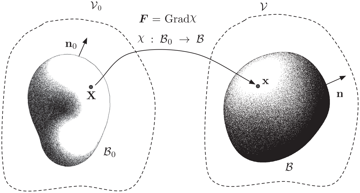
Consider a deformable body, the boundary or interior of which does not possess any distributed dipoles, occupying a three-dimensional region $\mathcal{B}$ lying inside another region $\mathcal{V}$ , as schematically depicted in Figure 1. We denote the region exterior to the body, relative to $\mathcal{V}$ , by $\mathcal{B}\prime$ so that $\mathcal{B}\prime =\mathcal{V}\backslash (\mathcal{B}\cup \partial \mathcal{B}).$ We assume that the body occupies a region ${\mathcal{B}}_0$ in its reference configuration while ${\mathcal{V}}_0$ is the referential region corresponding to $\mathcal{V}$ , as explained next. The points in regions ${\mathcal{B}}_0$ and $\mathcal{B}$ corresponding to the same material point of the body are naturally mapped into each other by the deformation function

$$\chi :{\mathcal{B}}_0\to \mathcal{B}.$$

(1)

To make sense of the referential (Lagrangian) description of fields in the current region $\mathcal{V}$ , but exterior to the body, in a meaningful manner, we also define an extension of the deformation function $\chi$ to the part of the region exterior to the body, such that sufficient continuity requirements are maintained; the latter region is denoted by

$${\mathcal{B}\prime }_0={\mathcal{V}}_0\backslash ({\mathcal{B}}_0\cup \partial {\mathcal{B}}_0).$$

Thus, by an abuse of notation, we assume an extension of mapping $\chi$ on a larger region, also denoted by $\chi$ , i.e.,

$$\chi :{\mathcal{V}}_0\to \mathcal{V}.$$

(2)

In typical situations in practice, it is assumed that $\partial {\mathcal{V}}_0$ and $\partial \mathcal{V}$ coincide (for instance, this is the scenario depicted in Fig. 1).

Figure 1.

Representation of the problem; the body is depicted in its reference and current configurations embedded in a volume $\mathcal{V}$ .

Following the standard notation in continuum mechanics, we define the deformation gradient for points in the reference configuration ${\mathcal{B}}_0$ and on its exterior relative to ${\mathcal{V}}_0$ as

$$\mathbf{F}:=\mathrm{Grad}\chi .$$

The extension of the natural definition of deformation and its gradient associated with $\chi$ on ${\mathcal{B}}_0$ to ${\mathcal{V}}_0$ permits us later to perform some useful manipulations on the reference configuration, as well as on the exterior of the body ${\mathcal{B}\prime }_0$ in the reference configuration.

The magnetic field vector, magnetic induction vector and magnetisation vector are denoted in the reference configuration as $(\mathbb{H},\mathbb{B},\mathbb{M})$ , respectively, and in the current configuration as $(\mathbb{h},\mathbb{b},\mathbb{m})$ , respectively. These three vector fields are related by the well-known constitutive relation

$$\mathbb{b}={\mu }_0\mathbb{h}+\mathbb{m}.$$

(3)

Further, the vector fields $(\mathbb{h},\mathbb{b},\mathbb{m})$ must satisfy the Maxwell’s equations

$$\mathrm{div}\mathbb{b}=0\mathrm{and}\mathrm{curl}\mathbb{h}=0\mathrm{in}\mathcal{B}\cup \mathcal{B}\prime .$$

(4)

The divergence-free and curl-free conditions (equation (4)) for $\mathbb{b}$ and $\mathbb{h}$ , respectively, lead to the existence of a magnetic potential (vector) field $\mathbb{a}$ and a magnetic potential (scalar) field $\varphi$ on $\mathcal{B}\cup \mathcal{B}\prime$ ; the corresponding expressions of $\mathbb{b}$ and $\mathbb{h}$ are given by

$$\mathbb{b}=\mathrm{curl}\mathbb{a},\mathbb{h}=-\mathrm{grad}\varphi .$$

(5)

Following tradition in continuum mechanics [37], let $J$ denote the determinant of the deformation gradient, i.e., $J=det\mathbf{F}$ (note that $J>0$ on ${\mathcal{B}}_0$ as well as on $\mathcal{B}{\prime }_0$ ). The referential (Lagrangian) counterparts of $\mathbb{b}$ and $\mathbb{h}$ , defined by

$$\mathbb{B}=J{\mathbf{F}}^{-1}\mathbb{b},\mathbb{H}={\mathbf{F}}^{\mathrm{T}}\mathbb{h},$$

(6)

naturally satisfy the Maxwell’s equations (equation (4)) in the reference configuration as

$$\mathrm{Div}\mathbb{B}=0\mathrm{and}\mathrm{Curl}\mathbb{H}=0\mathrm{in}{\mathcal{B}}_0\cup \mathcal{B}{\prime }_0.$$

(7)

Suitable referential (Lagrangian) counterparts of the magnetic vector potential and magnetic scalar potential (equation (5)) on ${\mathcal{B}}_0\cup \mathcal{B}{\prime }_0$ , based on the referential equations (equation (7)), are given by

$$\mathbb{B}=\mathrm{Curl}\mathbb{A},\mathbb{H}=-\mathrm{Grad}\mathrm{\Phi }.$$

(8)

Concerning notational issues, a typical point in ${\mathcal{B}}_0$ (as well as $\mathcal{B}{\prime }_0$ ) is denoted by $\mathit{X}$ , which is related (after deformation) to the point in $\mathcal{B}$ (or $\mathcal{B}\prime$ ) by the deformation function $\chi$ , assumed to be a sufficiently smooth mapping, such that $\mathit{x}=\chi (\mathit{X})$ and $\mathit{X}={\chi }^{-1}(\mathit{x})$ [37], i.e.,

$$\mathit{X}\mapsto \mathit{x},\mathit{x}\mapsto \mathit{X}.$$

(9)

It can be shown using tensor algebra and calculus that

$$\mathbb{A}(\mathit{X})={\mathbf{F}}^{\mathrm{T}}(\mathit{X})\mathbb{a}(\mathit{x}),\mathrm{\Phi }(\mathit{X})=\varphi (\mathit{x}),$$

(10)

for all $\mathit{X}\in {\mathcal{B}}_0\cup \mathcal{B}{\prime }_0$ . On substituting the transformations (equations (6)) into the constitutive relation (equation (3)), we obtain the relation

$$J^{-1}\mathbf{C}\mathbb{B}={\mu }_0\mathbb{H}+\mathbb{M},$$

(11)

where $\mathbb{M}$ denotes the referential (Lagrangian) magnetisation (per unit volume) vector field. Clearly, $\mathbb{M}$ is related to the current (spatial, Eulerian) magnetisation (per unit volume) vector field $\mathbb{m}$ by the definition (recall equation (9))

$$\mathbb{M}(\mathit{X}):={\mathbf{F}}^{\mathrm{T}}(\mathit{X})\mathbb{m}(\mathit{x}),$$

(12)

for all $\mathit{X}\in {\mathcal{B}}_0\cup \mathcal{B}{\prime }_0$ (as $\mathbb{m}$ is zero in $\mathcal{B}\prime$ , we also get vanishing $\mathbb{M}$ in $\mathcal{B}{\prime }_0$ ). From the point of view of practical applications motivated by physics-oriented models, it is also useful to define the magnetisation (per unit mass) $\overline{\mathbb{m}}:\mathcal{B}\to {\mathbb{R}}^3$ . It is easy to see that the defining relation is

$$\overline{\mathbb{m}}(\mathit{x}):=\rho (\mathit{x}{)}^{-1}\mathbb{m}(\mathit{x}),\mathit{x}\in \mathcal{B},$$

(13)

where $\rho$ stands for the mass density, i.e., a scalar field on $\mathcal{B}$ . The referential (Lagrangian) counterpart of the spatial field $\overline{\mathbb{m}}$ is denoted by $\overline{\mathbb{M}}$ , which is defined by

$$\overline{\mathbb{M}}(\mathit{X}):=J^{-1}(\mathit{X}){\mathbf{F}}^{\mathrm{T}}(\mathit{X})\overline{\mathbb{m}}(\mathit{x}),\mathit{X}\in {\mathcal{B}}_0.$$

(14)

Remark 1. When the density ${\rho }_0$ in the reference configuration is a constant, in particular for a homogeneous body, it is easy to see that $\overline{\mathbb{M}}$ and $\mathbb{M}$ are simply proportional (i.e., $\mathbb{M}={\rho }_0\overline{\mathbb{M}}$ as ${\rho }_0=\rho J$ ).

Holding the viewpoint of several practical applications where magnetoelastic materials are involved, in certain situations it is quite convenient to distinguish the externally applied fields and the fields generated as a result of the presence of the magnetoelastic body. In such a typical scenario, an external magnetic field ${\mathbb{h}}^{\mathrm{e}}$ is applied that results in the generation of a magnetic flux density ${\mathbb{b}}^{\mathrm{e}}$ with the relation

$${\mathbb{b}}^{\mathrm{e}}={\mu }_0{\mathbb{h}}^{\mathrm{e}},$$

(15)

where ${\mu }_0$ is the (constant) magnetic permeability of vacuum. The presence of the magnetoelastic body creates a perturbation (sometimes described as the self-field) in the magnetic field that is denoted by ${\mathbb{h}}^{\mathrm{s}}$ and a corresponding self-field for the magnetic flux vector denoted by ${\mathbb{b}}^{\mathrm{s}}$ [7].

Remark 2. In general, in this paper the decoration with superscript ‘s’ denotes the self-field or stray field while the superscript ‘e’ denotes the externally applied entity.

Thus, the total magnetic field and induction vector field are given by the sums

$$\mathbb{h}={\mathbb{h}}^{\mathrm{e}}+{\mathbb{h}}^{\mathrm{s}},\mathbb{b}={\mathbb{b}}^{\mathrm{e}}+{\mathbb{b}}^{\mathrm{s}}.$$

(16)

The relationship between the three magnetic vector fields ${\mathbb{b}}^{\mathrm{s}},{\mathbb{h}}^{\mathrm{s}}$ and the magnetisation per unit volume $\mathbb{m}$ is naturally given by

$${\mathbb{b}}^{\mathrm{s}}={\mu }_0{\mathbb{h}}^{\mathrm{s}}+\mathbb{m},$$

(17)

which holds on account of equations (15) and (16).

Remark 3. Concerning the units of the magnetisation vector $\mathbb{m}$ , we note that the definition of the magnetisation vector is not standardised in the literature and, depending on the choice of units, either one of $\mathbb{m}$ and ${\mu }_0\mathbb{m}$ have been used. Thus, the constitutive equation relating the three magnetic variables is also sometimes written as ${\mathbb{b}}^{\mathrm{s}}={\mu }_0[{\mathbb{h}}^{\mathrm{s}}+\mathbb{m}]$ for a different set of units. A detailed discussion on this topic can be found in [11].

3. First formulation based on magnetisation

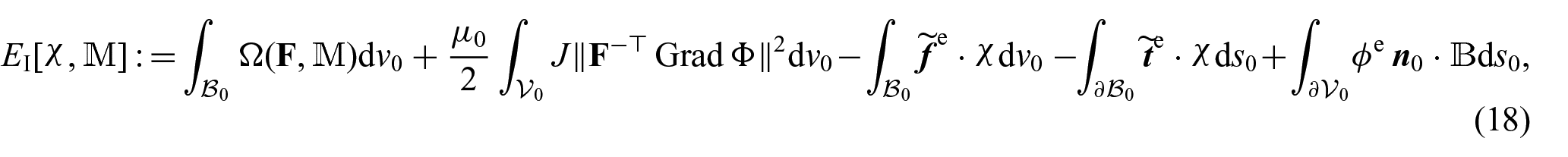
Consider the body ${\mathcal{B}}_0$ in its reference configuration (lying inside a containing space ${\mathcal{V}}_0$ ). Noting that $\mathbb{H}=-\mathrm{Grad}\mathrm{\Phi }$ by equation (8), it is assumed that the total potential energy of the system is a functional of the deformation $\chi$ (equations (1) and (2)) and the referential magnetisation $\mathbb{M}$ (equation (12)) with the explicit expression given by [31]

$$E_{\mathrm{I}}[\chi ,\mathbb{M}]:={\int }_{{\mathcal{B}}_0}\mathrm{\Omega }(\mathbf{F},\mathbb{M})\mathrm{d}{v}_0+\frac{{\mu }_0}{2}{\int }_{{\mathcal{V}}_0}J\parallel {\mathbf{F}}^{-\mathrm{T}}\mathrm{Grad}\mathrm{\Phi }{\parallel }^2\mathrm{d}{v}_0-{\int }_{{\mathcal{B}}_0}{\tilde{\mathit{f}}}^{\mathrm{e}}·\chi \mathrm{d}{v}_0-{\int }_{\partial {\mathcal{B}}_0}{\tilde{\mathit{t}}}^{\mathrm{e}}·\chi \mathrm{d}{s}_0+{\int }_{\partial {\mathcal{V}}_0}{\varphi }^{\mathrm{e}}{\mathit{n}}_0·\mathbb{B}\mathrm{d}{s}_0,$$

(18)

where $\mathrm{\Omega }$ is the (magnetoelastic) stored energy density per unit volume that depends on the deformation gradient $\mathbf{F}$ and the referential magnetisation vector $\mathbb{M}$ . The second term denotes the energy stored in the space due to the externally applied magnetic field $\mathbb{h}=-{\mathbf{F}}^{-\mathrm{T}}\mathrm{Grad}\mathrm{\Phi }$ . Integrals in equation (18) are defined on the reference configuration and the spatial fields are mapped to the reference configuration by using the mapping $\chi$ as placement. In this expression of the potential energy functional, it is assumed that ${\varphi }^{\mathrm{e}}$ stands for the externally applied magnetic potential on the boundary of the containing region ${\mathcal{V}}_0$ . Note that ${\tilde{\mathit{f}}}^{\mathrm{e}}$ is the body force (vector) field per unit volume while ${\tilde{\mathit{t}}}^{\mathrm{e}}$ is the applied traction (vector) field due to dead loads at the boundary of the body in its current configuration; here, also recall the notation described in Remark 2.

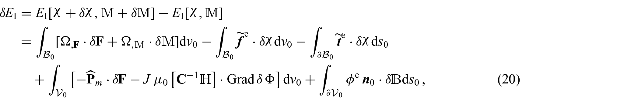
3.1. Equilibrium: first variation

To describe the state of magnetoelastic equilibrium, the particular deformation $\chi$ and magnetisation $\mathbb{M}$ at such an equilibrium corresponds to an extremum point of $E_1$ , that is, when the first variation of the potential energy functional vanishes. In other words, it is assumed that $\chi$ and $\mathbb{M}$ satisfy

$$\delta E_{\mathrm{I}}\equiv \delta E_{\mathrm{I}}[\chi ,\mathbb{M};(\delta \chi ,\delta \mathbb{M})]=0,$$

(19)

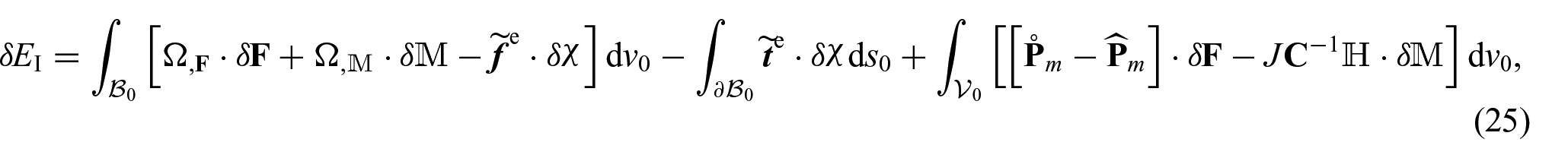
for arbitrary but admissible variations $\delta \chi$ and $\delta \mathbb{M}$ . The variation of the potential energy functional $E_{\mathrm{I}}$ up to the first order is given by

$$\begin{array}{c}\delta E_{\mathrm{I}}=E_{\mathrm{I}}[\chi +\delta \chi ,\mathbb{M}+\delta \mathbb{M}]-E_{\mathrm{I}}[\chi ,\mathbb{M}]\hfill \\ ={\int }_{{\mathcal{B}}_0}[{\mathrm{\Omega }}_{,\mathbf{F}}·\delta \mathbf{F}+{\mathrm{\Omega }}_{,\mathbb{M}}·\delta \mathbb{M}]\mathrm{d}{v}_0-{\int }_{{\mathcal{B}}_0}{\tilde{\mathit{f}}}^{\mathrm{e}}·\delta \chi \mathrm{d}{v}_0-{\int }_{\partial {\mathcal{B}}_0}{\tilde{\mathit{t}}}^{\mathrm{e}}·\delta \chi \mathrm{d}{s}_0\hfill \\ +{\int }_{{\mathcal{V}}_0}[-{\hat{\mathbf{P}}}_m·\delta \mathbf{F}-J{\mu }_0\left[{\mathbf{C}}^{-1}\mathbb{H}\right]·\mathrm{Grad}\delta \mathrm{\Phi }]\mathrm{d}{v}_0+{\int }_{\partial {\mathcal{V}}_0}{\varphi }^{\mathrm{e}}{\mathit{n}}_0·\delta \mathbb{B}\mathrm{d}{s}_0,\hfill \end{array}$$

(20)

where ${\hat{\mathbf{P}}}_m$ is a tensor field defined by

$${\hat{\mathbf{P}}}_m={\mu }_{0}J[-\frac{1}{2}[{\mathbf{F}}^{-\mathrm{T}}\mathbb{H}]·[{\mathbf{F}}^{-\mathrm{T}}\mathbb{H}]\mathbf{I}+[{\mathbf{F}}^{-\mathrm{T}}\mathbb{H}]\otimes [{\mathbf{F}}^{-\mathrm{T}}\mathbb{H}]]{\mathbf{F}}^{-\mathrm{T}},$$

(21)

where $\mathbf{I}$ is the identity tensor. We are able to understand the physical nature of ${\hat{\mathbf{P}}}_m$ by noticing that, in the region $\mathcal{B}{\prime }_0$ exterior to the body, the magnetisation $\mathbb{M}=0$ ; this results in ${\hat{\mathbf{P}}}_m={\mathbf{P}}_m$ , where ${\mathbf{P}}_m$ denotes the well-known Maxwell stress tensor defined by

$${\mathbf{P}}_m:=\frac{1}{{\mu }_{0}J}[[\mathbf{F}\mathbb{B}]\otimes [\mathbf{F}\mathbb{B}]-\frac{1}{2}[\mathbf{F}\mathbb{B}]·[\mathbf{F}\mathbb{B}]\mathbf{I}]{\mathbf{F}}^{-\mathrm{T}}.$$

(22)

To further simplify the first variation expression (equation (20)), we apply the divergence theorem on the last term and use the condition from a variation of equation (7) that $\mathrm{Div}(\delta \mathbb{B})=0$ to get

$$\begin{array}{c}{\int }_{\partial {\mathcal{V}}_0}{\mathit{n}}_0·\varphi \delta \mathbb{B}\mathrm{d}{s}_0={\int }_{{\mathcal{V}}_0}\mathrm{Div}\left(\varphi \delta \mathbb{B}\right)\mathrm{d}{v}_0={\int }_{{\mathcal{V}}_0}\mathrm{Grad}(\varphi )·\delta \mathbb{B}\mathrm{d}{v}_0\hfill \\ =-{\int }_{{\mathcal{V}}_0}\mathbb{H}·\delta \mathbb{B}\mathrm{d}{v}_0.\hfill \end{array}$$

(23)

At this point, we recall several identities for variations of $\mathbf{C},J$ , etc., from Appendix B. Using the constitutive relation (equation (11)), an increment of magnetic induction $\mathbb{B}$ up to first order can be written as

$$\delta \mathbb{B}=[[{\mathbf{F}}^{-\mathrm{T}}·\delta \mathbf{F}]\mathbf{I}-{\mathbf{C}}^{-1}{\left[\delta \mathbf{F}\right]}^{\mathrm{T}}\mathbf{F}-{\mathbf{F}}^{-1}\left[\delta \mathbf{F}\right]]\mathbb{B}-{\mu }_{0}J{\mathbf{C}}^{-1}\mathrm{Grad}\delta \mathrm{\Phi }+J{\mathbf{C}}^{-1}\delta \mathbb{M}.$$

(24)

On substituting equations (23) and (24) in the last term of equation (20), we thus obtain

$$\delta E_{\mathrm{I}}={\int }_{{\mathcal{B}}_0}[{\mathrm{\Omega }}_{,\mathbf{F}}·\delta \mathbf{F}+{\mathrm{\Omega }}_{,\mathbb{M}}·\delta \mathbb{M}-{\tilde{\mathit{f}}}^{\mathrm{e}}·\delta \chi ]\mathrm{d}{v}_0-{\int }_{\partial {\mathcal{B}}_0}{\tilde{\mathit{t}}}^{\mathrm{e}}·\delta \chi \mathrm{d}{s}_0+{\int }_{{\mathcal{V}}_0}[[{\stackrel{°}{\mathbf{P}}}_m-{\hat{\mathbf{P}}}_m]·\delta \mathbf{F}-J{\mathbf{C}}^{-1}\mathbb{H}·\delta \mathbb{M}]\mathrm{d}{v}_0,$$

(25)

where we have defined the tensor

$$\begin{array}{c}{\stackrel{°}{\mathbf{P}}}_m:=[-[\mathbb{B}·\mathbb{H}]\mathbf{I}+[\mathbf{F}\mathbb{B}]\otimes \left[{\mathbf{F}}^{-\mathrm{T}}\mathbb{H}\right]+\left[{\mathbf{F}}^{-\mathrm{T}}\mathbb{H}\right]\otimes [\mathbf{F}\mathbb{B}]]{\mathbf{F}}^{-\mathrm{T}}\hfill \\ =2{\hat{\mathbf{P}}}_m+J[-[{\mathbf{C}}^{-1}\mathbb{M}·\mathbb{H}]\mathbf{I}+\left[{\mathbf{F}}^{-\mathrm{T}}\mathbb{M}\right]\otimes \left[{\mathbf{F}}^{-\mathrm{T}}\mathbb{H}\right]+\left[{\mathbf{F}}^{-\mathrm{T}}\mathbb{H}\right]\otimes \left[{\mathbf{F}}^{-\mathrm{T}}\mathbb{M}\right]]{\mathbf{F}}^{-\mathrm{T}}.\hfill \end{array}$$

(26)

As observed, $\mathbb{M}=0$ in the region ${\mathcal{B}\prime }_0$ , which leads to ${\stackrel{°}{\mathbf{P}}}_m=2{\mathbf{P}}_m$ .

On splitting the (third term) integral over ${\mathcal{V}}_0$ in equation (25) to a sum of the integrals on disjoint regions ${\mathcal{B}}_0$ and ${\mathcal{B}\prime }_0$ , we obtain

$$\delta E_{\mathrm{I}}={\int }_{{\mathcal{B}}_0}[[{\mathrm{\Omega }}_{\mathbf{F}}+{\stackrel{°}{\mathbf{P}}}_m-{\hat{\mathbf{P}}}_m]·\delta \mathbf{F}-{\tilde{\mathit{f}}}^{\mathrm{e}}·\delta \chi +[{\mathrm{\Omega }}_{,\mathbb{M}}-J{\mathbf{C}}^{-1}\mathbb{H}]·\delta \mathbb{M}]\mathrm{d}{v}_0-{\int }_{\partial {\mathcal{B}}_0}{\tilde{\mathit{t}}}^{\mathrm{e}}·\delta \chi \mathrm{d}{s}_0+{\int }_{{\mathcal{B}\prime }_0}{\mathbf{P}}_m·\delta \mathbf{F}\mathrm{d}{v}_0.$$

This is rewritten with the use of the divergence theorem as

$$\begin{array}{c}\delta E_{\mathrm{I}}={\int }_{{\mathcal{B}}_0}[-[\mathrm{Div}({\mathrm{\Omega }}_{,\mathbf{F}}+{\stackrel{°}{\mathbf{P}}}_m-{\hat{\mathbf{P}}}_m)+{\tilde{\mathit{f}}}^{\mathrm{e}}]·\delta \chi +[{\mathrm{\Omega }}_{,\mathbb{M}}-J{\mathbf{C}}^{-1}\mathbb{H}]·\delta \mathbb{M}]\mathrm{d}{v}_0\hfill \\ +{\int }_{\partial {\mathcal{B}}_0}[[[{\mathrm{\Omega }}_{,\mathbf{F}}+{\stackrel{°}{\mathbf{P}}}_m-{\hat{\mathbf{P}}}_m]{|}_{-}-{\mathbf{P}}_m{|}_{+}]{\mathit{n}}_0-{\tilde{\mathit{t}}}^{\mathrm{e}}]·\delta \chi \mathrm{d}{s}_0\hfill \\ -{\int }_{{\mathcal{B}\prime }_0}\mathrm{Div}{\mathbf{P}}_m·\delta \chi \mathrm{d}{v}_0+{\int }_{\partial {\mathcal{V}}_0}{\mathbf{P}}_m{\mathit{n}}_0·\delta \chi \mathrm{d}{s}_0.\hfill \end{array}$$

Following the traditional definition, at this point, by virtue of inspection of the form of the first variation of the potential energy functional, we define the first Piola–Kirchhoff stress in the body as

$$\mathbf{P}:={\mathrm{\Omega }}_{,\mathbf{F}}+{\stackrel{°}{\mathbf{P}}}_m-{\hat{\mathbf{P}}}_m,\mathrm{in}{\mathcal{B}}_0,$$

(27)

while we have the natural stress tensor, i.e., the Maxwell stress, $\mathbf{P}={\mathbf{P}}_m$ defined by equation (22) exterior to the body, i.e., in ${\mathcal{B}\prime }_0$ .

Remark 4. The Cauchy stress $\sigma$ in the body is related to the first Piola–Kirchhoff stress $\mathbf{P}$ by the Piola transform as $\sigma \mathrm{cof}(\mathbf{F})=\mathbf{P}$ ; this is also sometimes referred to as Nanson’s relation. On using equation (6) and the tensor field stated as equation (22), the counterpart ${\sigma }_m$ of the Cauchy stress $\sigma$ in $\mathcal{B}\prime$ (vacuum) is given by the expression

$$\sigma ={\sigma }_m=\frac{1}{{\mu }_0}[\mathbb{b}\otimes \mathbb{b}-\frac{1}{2}[\mathbb{b}·\mathbb{b}]\mathbf{I}]\mathrm{in}\mathcal{B}\prime .$$

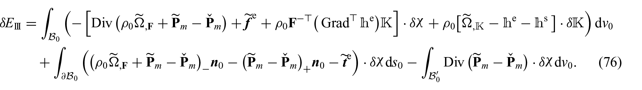
On applying equation (19) to the first variation, the coefficients appearing with the arbitrary variations $\delta \chi$ and $\delta \mathbb{M}$ should also vanish for the requirement that $\delta E_{\mathrm{I}}$ must be zero at equilibrium (i.e., $\chi ,\mathbb{M}$ corresponding to an extremum point of $E$ ). Vanishing of the coefficients of $\delta \mathbb{M}$ results in the following constitutive relation between $\mathbb{H}$ and $\mathbb{M}$ :

$$\mathbb{H}=J^{-1}\mathbf{C}{\mathrm{\Omega }}_{,\mathbb{M}}\mathrm{in}{\mathcal{B}}_0.$$

(28)

On substituting this expression for $\mathbb{H}$ in equations (21), (26) and (27), the total first Piola–Kirchhoff stress can be rewritten in terms of the independent quantities $\mathbf{F}$ and $\mathbb{M}$ as

$$\mathbf{P}={\mathrm{\Omega }}_{,\mathbf{F}}+{\stackrel{°}{\mathbf{P}}}_m-{\hat{\mathbf{P}}}_m$$

(29)

$$\begin{array}{c}={\mathrm{\Omega }}_{,\mathbf{F}}+{\mu }_0{J}^{-1}[-\frac{1}{2}{\mathrm{\Omega }}_{,\mathbb{M}}·[\mathbf{C}{\mathrm{\Omega }}_{,\mathbb{M}}]\mathbf{I}+\mathbf{F}{\mathrm{\Omega }}_{,\mathbb{M}}\otimes [\mathbf{F}{\mathrm{\Omega }}_{,\mathbb{M}}]]{\mathbf{F}}^{-\mathrm{T}}\hfill \\ +[-[\mathbb{M}·{\mathrm{\Omega }}_{,\mathbb{M}}]\mathbf{I}+{\mathbf{F}}^{-\mathrm{T}}\mathbb{M}\otimes \mathbf{F}{\mathrm{\Omega }}_{,\mathbb{M}}+\mathbf{F}{\mathrm{\Omega }}_{,\mathbb{M}}\otimes {\mathbf{F}}^{-\mathrm{T}}\mathbb{M}]{\mathbf{F}}^{-\mathrm{T}}.\hfill \end{array}$$

(30)

Also

$$\mathbf{P}=J(J^{-1}{\mathrm{\Omega }}_{,\mathbf{F}}{\mathbf{F}}^{\mathrm{T}}+\mathbb{h}\otimes \mathbb{b}-\frac{{\mu }_0}{2}(\mathbb{h}·\mathbb{h})\mathbf{I}+\{\mathbb{m}\otimes \mathbb{h}-(\mathbb{m}·\mathbb{h})\mathbf{I}\}){\mathbf{F}}^{-\mathrm{T}},$$

which differs from that given by [13] (see their equation (2.26) and Section 6.3 of this paper), owing to the presence of the terms in the curly brackets. Vanishing of the coefficients of $\delta \chi$ results in the following equations:

$$\mathrm{Div}\mathbf{P}+{\tilde{\mathit{f}}}^{\mathrm{e}}=0\mathrm{in}{\mathcal{B}}_0,$$

(31a)

$$\mathrm{Div}\mathbf{P}=0\mathrm{in}{\mathcal{B}\prime }_0,$$

(31b)

$$\left[\left[\mathbf{P}\right]\right]{\mathit{n}}_0+{\tilde{\mathit{t}}}^{\mathrm{e}}=0\mathrm{on}\partial {\mathcal{B}}_0,$$

(31c)

$$\mathbf{P}{\mathit{n}}_0=0\mathrm{on}\partial {\mathcal{V}}_0.$$

(31d)

Here, $\left[[\{·\}]\right]=\{·{\}}_{+}-\{·{\}}_{-}$ with the plus sign representing that side of the boundary (surface) that is reached along the unit outward normal vector.

Remark 5. We note that in this formulation based on the magnetisation vector, we have to a-priori use both the Maxwell’s equations (equation (7)) to impose conditions on $\mathbb{B}$ and $\mathbb{H}$ unlike the two formulations based on $\mathbb{B}$ and $\mathbb{H}$ presented in Appendices C and D, in which one condition is imposed and the other is derived. Also, unlike those two formulations, stress does not have a simple expression of being a derivative of the stored energy density with respect to the deformation gradient tensor. The procedure implies the constitutive relation (equation (28)) between $\mathbb{H}$ and $\mathbb{M}$ .

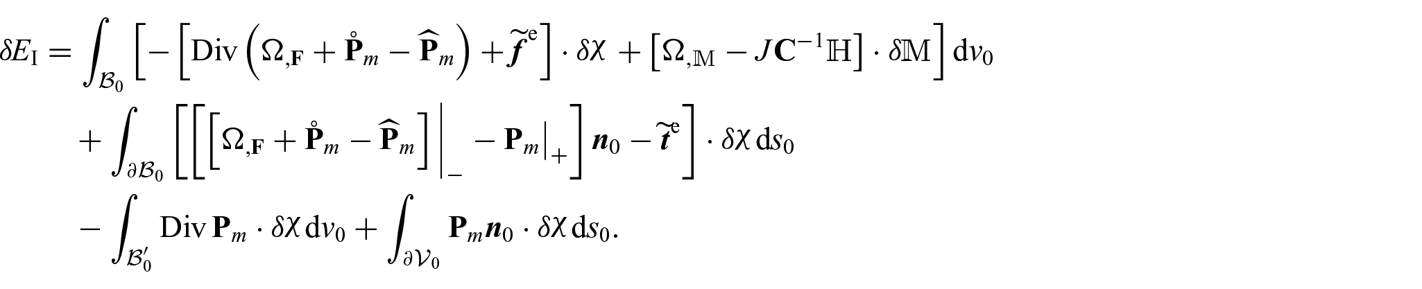
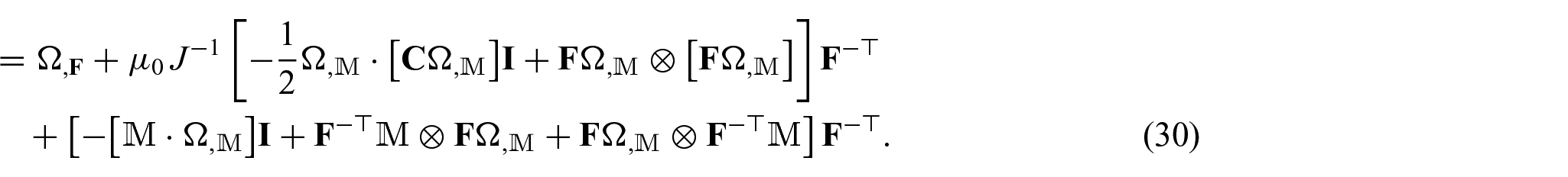
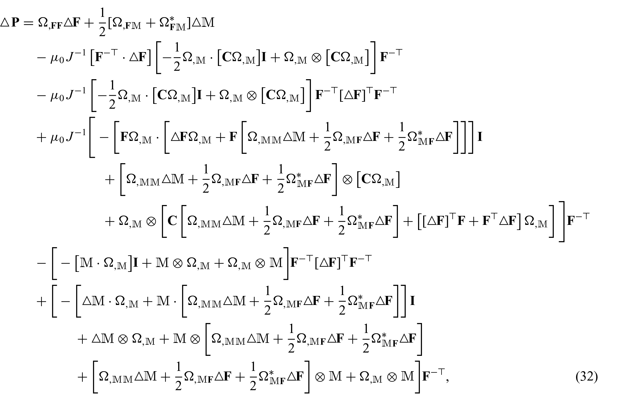
3.2. Perturbation of equilibrium equation at critical point

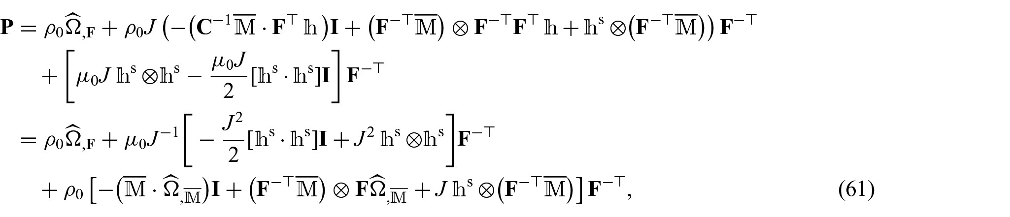
In terms of the variations $\mathrm{\Delta }\chi$ and $\mathrm{\Delta }\mathbb{M}$ , we find the perturbation in the first Piola–Kirchhoff stress using equation (30) as

$$\begin{array}{c}\mathrm{\Delta }\mathbf{P}={\mathrm{\Omega }}_{,\mathbf{FF}}\mathrm{\Delta }\mathbf{F}+\frac{1}{2}[{\mathrm{\Omega }}_{,\mathbf{F}\mathbb{M}}+{\mathrm{\Omega }}_{\mathbf{F}\mathbb{M}}^{*}]\mathrm{\Delta }\mathbb{M}\hfill \\ -{\mu }_0{J}^{-1}[{\mathbf{F}}^{-\mathrm{T}}·\mathrm{\Delta }\mathbf{F}][-\frac{1}{2}{\mathrm{\Omega }}_{,\mathbb{M}}·[\mathbf{C}{\mathrm{\Omega }}_{,\mathbb{M}}]\mathbf{I}+{\mathrm{\Omega }}_{,\mathbb{M}}\otimes [\mathbf{C}{\mathrm{\Omega }}_{,\mathbb{M}}]]{\mathbf{F}}^{-\mathrm{T}}\hfill \\ -{\mu }_0{J}^{-1}[-\frac{1}{2}{\mathrm{\Omega }}_{,\mathbb{M}}·[\mathbf{C}{\mathrm{\Omega }}_{,\mathbb{M}}]\mathbf{I}+{\mathrm{\Omega }}_{,\mathbb{M}}\otimes [\mathbf{C}{\mathrm{\Omega }}_{,\mathbb{M}}]]{\mathbf{F}}^{-\mathrm{T}}[\mathrm{\Delta }\mathbf{F}{]}^{\mathrm{T}}{\mathbf{F}}^{-\mathrm{T}}\hfill \\ +{\mu }_0{J}^{-1}[-[\mathbf{F}{\mathrm{\Omega }}_{,\mathbb{M}}·[\mathrm{\Delta }\mathbf{F}{\mathrm{\Omega }}_{,\mathbb{M}}+\mathbf{F}[{\mathrm{\Omega }}_{,\mathbb{M}\mathbb{M}}\mathrm{\Delta }\mathbb{M}+\frac{1}{2}{\mathrm{\Omega }}_{,\mathbb{M}\mathbf{F}}\mathrm{\Delta }\mathbf{F}+\frac{1}{2}{\mathrm{\Omega }}_{\mathbb{M}\mathbf{F}}^{*}\mathrm{\Delta }\mathbf{F}]]]\mathbf{I}\hfill \\ +[{\mathrm{\Omega }}_{,\mathbb{M}\mathbb{M}}\mathrm{\Delta }\mathbb{M}+\frac{1}{2}{\mathrm{\Omega }}_{,\mathbb{M}\mathbf{F}}\mathrm{\Delta }\mathbf{F}+\frac{1}{2}{\mathrm{\Omega }}_{\mathbb{M}\mathbf{F}}^{*}\mathrm{\Delta }\mathbf{F}]\otimes [\mathbf{C}{\mathrm{\Omega }}_{,\mathbb{M}}]\hfill \\ +{\mathrm{\Omega }}_{,\mathbb{M}}\otimes [\mathbf{C}[{\mathrm{\Omega }}_{,\mathbb{M}\mathbb{M}}\mathrm{\Delta }\mathbb{M}+\frac{1}{2}{\mathrm{\Omega }}_{,\mathbb{M}\mathbf{F}}\mathrm{\Delta }\mathbf{F}+\frac{1}{2}{\mathrm{\Omega }}_{\mathbb{M}\mathbf{F}}^{*}\mathrm{\Delta }\mathbf{F}]+[{[\mathrm{\Delta }\mathbf{F}]}^{\mathrm{T}}\mathbf{F}+{\mathbf{F}}^{\mathrm{T}}\mathrm{\Delta }\mathbf{F}]{\mathrm{\Omega }}_{,\mathbb{M}}]]{\mathbf{F}}^{-\mathrm{T}}\hfill \\ -[-[\mathbb{M}·{\mathrm{\Omega }}_{,\mathbb{M}}]\mathbf{I}+\mathbb{M}\otimes {\mathrm{\Omega }}_{,\mathbb{M}}+{\mathrm{\Omega }}_{,\mathbb{M}}\otimes \mathbb{M}]{\mathbf{F}}^{-\mathrm{T}}[\mathrm{\Delta }\mathbf{F}{]}^{\mathrm{T}}{\mathbf{F}}^{-\mathrm{T}}\hfill \\ +[-[\mathrm{\Delta }\mathbb{M}·{\mathrm{\Omega }}_{,\mathbb{M}}+\mathbb{M}·[{\mathrm{\Omega }}_{,\mathbb{M}\mathbb{M}}\mathrm{\Delta }\mathbb{M}+\frac{1}{2}{\mathrm{\Omega }}_{,\mathbb{M}\mathbf{F}}\mathrm{\Delta }\mathbf{F}+\frac{1}{2}{\mathrm{\Omega }}_{\mathbb{M}\mathbf{F}}^{*}\mathrm{\Delta }\mathbf{F}]]\mathbf{I}\hfill \\ +\mathrm{\Delta }\mathbb{M}\otimes {\mathrm{\Omega }}_{,\mathbb{M}}+\mathbb{M}\otimes [{\mathrm{\Omega }}_{,\mathbb{M}\mathbb{M}}\mathrm{\Delta }\mathbb{M}+\frac{1}{2}{\mathrm{\Omega }}_{,\mathbb{M}\mathbf{F}}\mathrm{\Delta }\mathbf{F}+\frac{1}{2}{\mathrm{\Omega }}_{\mathbb{M}\mathbf{F}}^{*}\mathrm{\Delta }\mathbf{F}]\hfill \\ +[{\mathrm{\Omega }}_{,\mathbb{M}\mathbb{M}}\mathrm{\Delta }\mathbb{M}+\frac{1}{2}{\mathrm{\Omega }}_{,\mathbb{M}\mathbf{F}}\mathrm{\Delta }\mathbf{F}+\frac{1}{2}{\mathrm{\Omega }}_{\mathbb{M}\mathbf{F}}^{*}\mathrm{\Delta }\mathbf{F}]\otimes \mathbb{M}+{\mathrm{\Omega }}_{,\mathbb{M}}\otimes \mathbb{M}]{\mathbf{F}}^{-\mathrm{T}},\hfill \end{array}$$

(32)

where we have defined two third-order tensors ${\mathrm{\Omega }}_{\mathbf{F}\mathbb{M}}^{*}$ and ${\mathrm{\Omega }}_{\mathbb{M}\mathbf{F}}^{*}$ , which have the following property:

$$[{\mathrm{\Omega }}_{\mathbf{F}\mathbb{M}}^{*}\mathit{u}]·\mathbf{U}=[{\mathrm{\Omega }}_{,\mathbb{M}\mathbf{F}}\mathbf{U}]·\mathit{u},[{\mathrm{\Omega }}_{\mathbb{M}\mathbf{F}}^{*}\mathbf{U}]·\mathit{u}=[{\mathrm{\Omega }}_{,\mathbf{F}\mathbb{M}}\mathit{u}]·\mathbf{U},$$

(33)

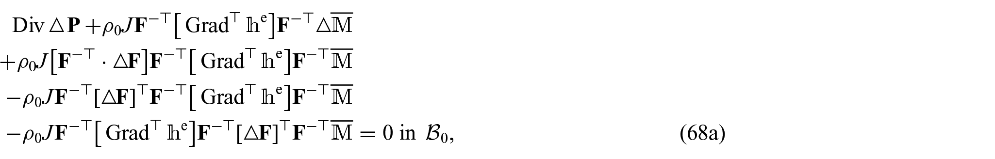
where $\mathit{u}$ is an arbitrary vector and $\mathbf{U}$ is an arbitrary second-order tensor. For the bifurcation analysis of critical point $(\chi ,\mathbb{M})$ , using equation (3.1), the perturbations $\mathrm{\Delta }\chi$ and $\mathrm{\Delta }\mathbb{M}$ in the equilibrium state need to satisfy the following partial differential equations and boundary conditions:

$$\mathrm{Div}\mathrm{\Delta }\mathbf{P}=0\mathrm{in}{\mathcal{B}}_0,$$

(34a)

$$\mathrm{Div}\mathrm{\Delta }\mathbf{P}=0\mathrm{in}\mathcal{B}{\prime }_0,$$

(34b)

$$\left[\left[\mathrm{\Delta }\mathbf{P}\right]\right]{\mathit{n}}_0=0\mathrm{on}\partial {\mathcal{B}}_0,$$

(34c)

$$\mathrm{\Delta }\mathbf{P}{\mathit{n}}_0=0\mathrm{on}\partial {\mathcal{V}}_0.$$

(34d)

This set of equations needs to be solved for the nontrivial unknown functions $(\mathrm{\Delta }\chi ,\mathrm{\Delta }\mathbb{M})$ describing the onset of bifurcation.

Remark 6. Perturbation in the Maxwell stress $\mathrm{\Delta }{\mathbf{P}}_m$ in $\mathcal{B}{\prime }_0$ in terms of $\mathrm{\Delta }\mathbf{F}$ and $\mathrm{\Delta }\mathbb{H}$ is given by equation (162). The boundary condition (equation (34c)) connects $\mathrm{\Delta }\mathbf{P}$ (equation (32)) and $\mathrm{\Delta }{\mathbf{P}}_m$ (equation (162)) through the constitutive relation (equation (28)) for $\mathbb{H}$ .

Remark 7. In the context of the first variation, as well as of the critical point perturbation, these expressions and equations are similar to those obtained in two other formulations based on $\mathbb{B}$ and $\mathbb{H}$ . These are summarised in Appendices C and D, where the derivations provided in [13] for the case of electroelastic materials are closely followed.

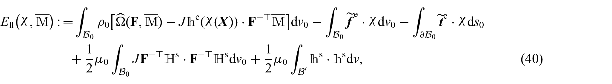
4. Second formulation based on magnetisation

Suppose that the physical space exterior to $\mathcal{B}$ is the entire space outside; in other words, we assume that

$$\mathcal{V}={\mathbb{R}}^3.$$

(35)

We consider that scenario when the potential energy functional depends on the magnetic energy stored in the entire space, due to the so-called stray field ${\mathbb{h}}^{\mathrm{s}}$ , and also includes a contribution of the work done by an external magnetic field ${\mathbb{h}}^{\mathrm{e}}$ on the magnetisation induced in the body. As a consequence of this, unlike the formulation presented in Section 3 and in Appendices C and D, we do not have any contribution from those terms that involve an integral on the boundary of the region exterior to the body, i.e., on $\partial \mathcal{V}$ . In particular, the total (magnetoelastic) stored energy $\overline{\mathcal{E}}$ in the considered system is the sum of the energy stored in the body and the stray magnetic field energy of the entire space. The explicit mathematical expression of the energy, as a functional of the deformation $\chi$ (equations (1) and (2)) and the spatial magnetisation $\overline{\mathbb{m}}$ (equations (13) and (14)), is given (per unit mass) by

$$\overline{\mathcal{E}}(\chi ,\overline{\mathbb{m}}):={\int }_{\mathcal{B}}\rho \overline{\hat{\mathrm{\Omega }}}(\mathbf{F},\overline{\mathbb{m}})\mathrm{d}v+{\int }_{{\mathbb{R}}^3}\frac{1}{2}{\mu }_0{\mathbb{h}}^{\mathrm{s}}·{\mathbb{h}}^{\mathrm{s}}\mathrm{d}v,$$

(36)

where we have defined $\overline{\hat{\mathrm{\Omega }}}$ as the Helmholtz energy (per unit mass). Following the physical nature of the stray fields, also by convention, it is assumed that the stray magnetic field ${\mathbb{h}}^{\mathrm{s}}$ decays (in a suitable manner) far away from the body, that is $\parallel {\mathbb{h}}^{\mathrm{s}}\parallel \to 0$ as $\parallel \mathit{x}\parallel \to \infty$ (recall that $\mathit{x}$ denotes the position vector in the current configuration).

The work done on the magnetoelastic body (the same as the negative of the potential energy of the applied dead loading) by externally applied mechanical and magnetic forces is given by [13]

$${\int }_{\mathcal{B}}\rho {\mathbb{h}}^{\mathrm{e}}·\overline{\mathbb{m}}\mathrm{d}v+{\int }_{\mathcal{B}}\rho {\mathit{f}}^{\mathrm{e}}·\chi \mathrm{d}v+{\int }_{\partial \mathcal{B}}{\mathit{t}}^{\mathrm{e}}·\chi \mathrm{d}s,$$

(37)

where ${\mathit{f}}^{\mathrm{e}}$ denotes the body force (per unit mass) and ${\mathit{t}}^{\mathrm{e}}$ denotes the mechanical traction (per unit area of the current configuration), while the first term is identified as the Zeeman energy [38]. It is emphasised that ${\mathit{f}}^{\mathrm{e}},{\mathit{t}}^{\mathrm{e}}$ and ${\mathbb{h}}^{\mathrm{e}}$ are external dead loads.

Using equations (36) and (37), the potential energy $\overline{E_{\mathrm{II}}}$ of the system comprising the body and the surrounding space is then given by $\overline{\mathcal{E}}$ minus the magnetoelastic work done, i.e.,

$$\overline{E_{\mathrm{II}}}(\chi ,\overline{\mathbb{m}}):={\int }_{\mathcal{B}}[\rho \overline{\hat{\mathrm{\Omega }}}(\mathbf{F},\overline{\mathbb{m}})-{\mathbb{h}}^{\mathrm{e}}·(\rho \overline{\mathbb{m}})-\rho {\mathit{f}}^{\mathrm{e}}·\chi ]\mathrm{d}v-{\int }_{\partial \mathcal{B}}{\mathit{t}}^{\mathrm{e}}·\chi \mathrm{d}s+\frac{1}{2}{\mu }_0{\int }_{\mathcal{B}}{\mathbb{h}}^{\mathrm{s}}·{\mathbb{h}}^{\mathrm{s}}\mathrm{d}v+\frac{1}{2}{\mu }_0{\int }_{\mathcal{B}\prime }{\mathbb{h}}^{\mathrm{s}}·{\mathbb{h}}^{\mathrm{s}}\mathrm{d}v.$$

(38)

Remark 8. We emphasise that even though the Eulerian expression of the potential energy $\overline{E_{\mathrm{II}}}$ is the same as that provided by Kankanala and Triantafyllidis [13], our formulation is markedly different from theirs, since we consider the mechanical deformation $\chi$ and the magnetisation in the body $\overline{\mathbb{m}}$ as the only two unknown fields of the problem. Moreover, our referential formulation is quite different from that of [13], as discussed next. In terms of $\chi$ and $\overline{\mathbb{m}}$ , the magnetic vector field ${\mathbb{b}}^{\mathrm{s}}$ can be found by employing the Maxwell’s equations stated in Section 2. As

$${\mathbb{b}}^{\mathrm{s}}={\mu }_0{\mathbb{h}}^{\mathrm{s}}+\rho \overline{\mathbb{m}}$$

(39)

and ${\mathbb{h}}^{\mathrm{s}}=-\mathrm{grad}{\varphi }^{\mathrm{s}}$ by equations (17) and (13), while ${\varphi }^{\mathrm{s}}$ is found from the condition (equation (4)), i.e., $\mathrm{div}{\mathbb{b}}^{\mathrm{s}}=0$ , that ${\mathbb{b}}^{\mathrm{s}}$ satisfies.

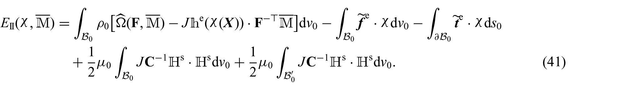
It is preferable to write the potential energy in equation (38) in the reference (Lagrangian) configuration, i.e., all field variables are functions of the reference position vector $\mathit{X}$ instead of the current position vector $\mathit{x}$ ( $=\chi (\mathit{X})$ ).

The Helmholtz energy function $\overline{\hat{\mathrm{\Omega }}}(\mathbf{F},\overline{\mathbb{m}})$ in equation (38) is mapped to $\hat{\mathrm{\Omega }}(\mathbf{F},\overline{\mathbb{M}})$ (recall equation (9)), i.e.,

$$\overline{\hat{\mathrm{\Omega }}}(\mathbf{F}({\chi }^{-1}(\mathit{x}),\overline{\mathbb{m}}(\mathit{x}))=\hat{\mathrm{\Omega }}(\mathbf{F}(\mathit{X}),\overline{\mathbb{M}}(\mathit{X})),\mathit{X}\in {\mathcal{B}}_0.$$

It is emphasised that the field ${\mathbb{h}}^{\mathrm{e}}$ depends directly on the spatial location $\mathit{x}$ (unlike ${\mathit{f}}^{\mathrm{e}}$ ) and is therefore explicitly mentioned as such.

Recall equation (13) and Remark 1, and in particular the relations

$$\mathbb{m}=\rho \overline{\mathbb{m}}=\rho J{\mathbf{F}}^{-\mathrm{T}}\overline{\mathbb{M}}={\rho }_0{\mathbf{F}}^{-\mathrm{T}}\overline{\mathbb{M}}={\mathbf{F}}^{-\mathrm{T}}\mathbb{M}\mathrm{and}\mathbb{M}={\rho }_0\overline{\mathbb{M}}.$$

Using these transformations, we can redefine the expression of the potential energy functional (equation (38)) in a referential description as

$$\begin{array}{c}{E}_{\mathrm{II}}(\chi ,\overline{\mathbb{M}}):={\int }_{{\mathcal{B}}_0}{\rho }_0[\hat{\mathrm{\Omega }}(\mathbf{F},\overline{\mathbb{M}})-J{\mathbb{h}}^{\mathrm{e}}(\chi (\mathit{X}))·{\mathbf{F}}^{-\mathrm{T}}\overline{\mathbb{M}}]\mathrm{d}{v}_0-{\int }_{{\mathcal{B}}_0}{\tilde{\mathit{f}}}^{\mathrm{e}}·\chi \mathrm{d}{v}_0-{\int }_{\partial {\mathcal{B}}_0}{\tilde{\mathit{t}}}^{\mathrm{e}}·\chi \mathrm{d}{s}_0\hfill \\ +\frac{1}{2}{\mu }_0{\int }_{{\mathcal{B}}_0}J{\mathbf{F}}^{-\mathrm{T}}{\mathbb{H}}^{\mathrm{s}}·{\mathbf{F}}^{-\mathrm{T}}{\mathbb{H}}^{\mathrm{s}}\mathrm{d}{v}_0+\frac{1}{2}{\mu }_0{\int }_{\mathcal{B}\prime }{\mathbb{h}}^{\mathrm{s}}·{\mathbb{h}}^{\mathrm{s}}\mathrm{d}v,\hfill \end{array}$$

(40)

where ${\tilde{\mathit{t}}}^{\mathrm{e}}$ is the force per unit area of the current configuration placed on the reference configuration, i.e., ${\tilde{\mathit{t}}}^{\mathrm{e}}(\mathit{X})\mathrm{d}{s}_0={\mathit{t}}^{\mathrm{e}}(\mathit{x})\mathrm{d}s,\mathit{X}\in \partial {\mathcal{B}}_0$ . Also, the body force per unit volume ${\tilde{\mathit{f}}}^{\mathrm{e}}$ on the reference configuration is related to ${\mathit{f}}^{\mathrm{e}}$ by ${\tilde{\mathit{f}}}^{\mathrm{e}}(\mathit{X})\mathrm{d}{v}_0=\rho {\mathit{f}}^{\mathrm{e}}(\mathit{x})\mathrm{d}v,\mathit{X}\in {\mathcal{B}}_0$ . In the first term of equation (40), we have highlighted the dependence on $\mathit{X}$ for additional clarity.

Recall that the extension of $\chi$ to $\mathcal{B}{\prime }_0$ is also denoted by $\chi$ and that the mapping $\chi$ is sufficiently smooth and it maps $\partial {\mathcal{B}}_0$ to $\partial \mathcal{B}$ such that it identifies with $\chi$ in that region and its gradient $\mathbf{F}$ identifies with the deformation gradient $\mathbf{F}$ of $\chi$ on the common boundary $\partial {\mathcal{B}}_0$ . In vacuum far from $\partial {\mathcal{B}}_0$ , the deformation gradient $\mathbf{F}$ can very well be assumed to be identity for convenience. We can rewrite the last term of the potential energy in equation (40) so that the entire expression becomes

$$\begin{array}{c}{E}_{\mathrm{II}}(\chi ,\overline{\mathbb{M}})={\int }_{{\mathcal{B}}_0}{\rho }_0[\hat{\mathrm{\Omega }}(\mathbf{F},\overline{\mathbb{M}})-J{\mathbb{h}}^{\mathrm{e}}(\chi (\mathit{X}))·{\mathbf{F}}^{-\mathrm{T}}\overline{\mathbb{M}}]\mathrm{d}{v}_0-{\int }_{{\mathcal{B}}_0}{\tilde{\mathit{f}}}^{\mathrm{e}}·\chi \mathrm{d}{v}_0-{\int }_{\partial {\mathcal{B}}_0}{\tilde{\mathit{t}}}^{\mathrm{e}}·\chi \mathrm{d}{s}_0\hfill \\ +\frac{1}{2}{\mu }_0{\int }_{{\mathcal{B}}_0}J{\mathbf{C}}^{-1}{\mathbb{H}}^{\mathrm{s}}·{\mathbb{H}}^{\mathrm{s}}\mathrm{d}{v}_0+\frac{1}{2}{\mu }_0{\int }_{\mathcal{B}{\prime }_0}J{\mathbf{C}}^{-1}{\mathbb{H}}^{\mathrm{s}}·{\mathbb{H}}^{\mathrm{s}}\mathrm{d}{v}_0.\hfill \end{array}$$

(41)

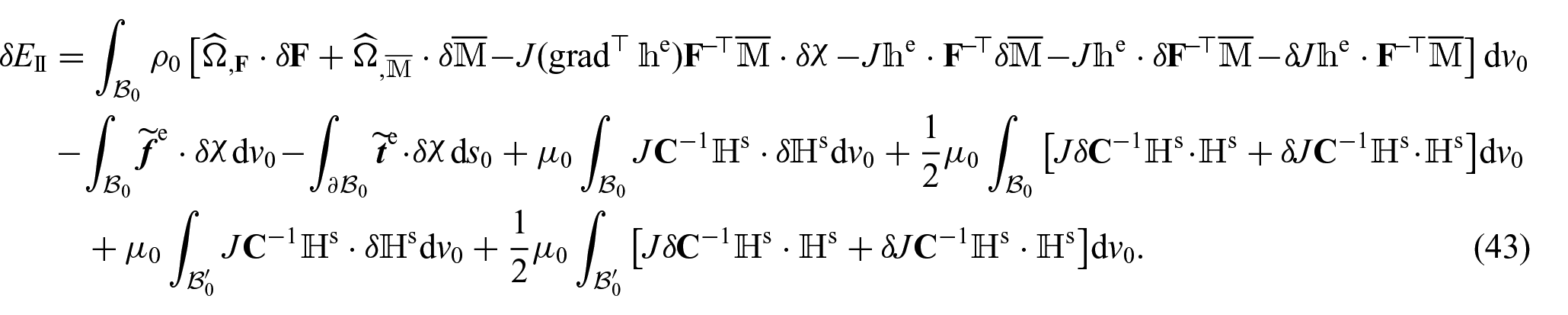
4.1. Equilibrium: first variation

On using the expressions for increments,

$$E_{\mathrm{II}}(\chi +\delta \chi ,\overline{\mathbb{M}}+\delta \overline{\mathbb{M}})-E_{\mathrm{II}}(\chi ,\overline{\mathbb{M}})=\delta E_{\mathrm{II}}(\chi ,\overline{\mathbb{M}})[\delta \chi ,\delta \overline{\mathbb{M}}]+\frac{1}{2}{\delta }^2{E}_{\mathrm{II}}(\chi ,\overline{\mathbb{M}})[\delta \chi ,\delta \overline{\mathbb{M}}]+o_2[\delta \chi ,\delta \overline{\mathbb{M}}],$$

(42)

where $o_2[\delta \chi ,\delta \overline{\mathbb{M}}]$ are the terms of order higher than two in $\delta \chi$ and $\delta \overline{\mathbb{M}}$ ; $\delta E_{\mathrm{II}}$ and ${\delta }^2{E}_{\mathrm{II}}$ are the first and the second variations of $E_{\mathrm{II}}$ , respectively.

The first variation $\delta E_{\mathrm{II}}[\delta \chi ,\delta \overline{\mathbb{M}}]$ , written simply as $\delta E_{\mathrm{II}}$ , is given by

$$\begin{array}{c}\delta E_{\mathrm{II}}={\int }_{{\mathcal{B}}_0}{\rho }_0[{\hat{\mathrm{\Omega }}}_{,\mathbf{F}}·\delta \mathbf{F}+{\hat{\mathrm{\Omega }}}_{,\overline{\mathbb{M}}}·\delta \overline{\mathbb{M}}-J(\mathrm{gra}{\mathrm{d}}^{\mathrm{T}}{\mathbb{h}}^{\mathrm{e}}){\mathbf{F}}^{-\mathrm{T}}\overline{\mathbb{M}}·\delta \chi -J{\mathbb{h}}^{\mathrm{e}}·{\mathbf{F}}^{-\mathrm{T}}\delta \overline{\mathbb{M}}-J{\mathbb{h}}^{\mathrm{e}}·\delta {\mathbf{F}}^{-\mathrm{T}}\overline{\mathbb{M}}-\delta J{\mathbb{h}}^{\mathrm{e}}·{\mathbf{F}}^{-\mathrm{T}}\overline{\mathbb{M}}]\mathrm{d}{v}_0\hfill \\ -{\int }_{{\mathcal{B}}_0}{\tilde{\mathit{f}}}^{\mathrm{e}}·\delta \chi \mathrm{d}{v}_0-{\int }_{\partial {\mathcal{B}}_0}{\tilde{\mathit{t}}}^{\mathrm{e}}·\delta \chi \mathrm{d}{s}_0+{\mu }_0{\int }_{{\mathcal{B}}_0}J{\mathbf{C}}^{-1}{\mathbb{H}}^{\mathrm{s}}·\delta {\mathbb{H}}^{\mathrm{s}}\mathrm{d}{v}_0+\frac{1}{2}{\mu }_0{\int }_{{\mathcal{B}}_0}[J\delta {\mathbf{C}}^{-1}{\mathbb{H}}^{\mathrm{s}}·{\mathbb{H}}^{\mathrm{s}}+\delta J{\mathbf{C}}^{-1}{\mathbb{H}}^{\mathrm{s}}·{\mathbb{H}}^{\mathrm{s}}]\mathrm{d}{v}_0\hfill \\ +{\mu }_0{\int }_{\mathcal{B}{\prime }_0}J{\mathbf{C}}^{-1}{\mathbb{H}}^{\mathrm{s}}·\delta {\mathbb{H}}^{\mathrm{s}}\mathrm{d}{v}_0+\frac{1}{2}{\mu }_0{\int }_{\mathcal{B}{\prime }_0}[J\delta {\mathbf{C}}^{-1}{\mathbb{H}}^{\mathrm{s}}·{\mathbb{H}}^{\mathrm{s}}+\delta J{\mathbf{C}}^{-1}{\mathbb{H}}^{\mathrm{s}}·{\mathbb{H}}^{\mathrm{s}}]\mathrm{d}{v}_0.\hfill \end{array}$$

(43)

Using the identities for variations of $\mathbf{C},J$ from Appendix B,

$$\frac{1}{2}{\mu }_0{\int }_{{\mathcal{B}}_0}[J\delta {\mathbf{C}}^{-1}{\mathbb{H}}^{\mathrm{s}}·{\mathbb{H}}^{\mathrm{s}}+\delta J{\mathbf{C}}^{-1}{\mathbb{H}}^{\mathrm{s}}·{\mathbb{H}}^{\mathrm{s}}]\mathrm{d}{v}_0={\int }_{{\mathcal{B}}_0}[-{\stackrel{⌣}{\mathbf{P}}}_m·\delta \mathbf{F}]\mathrm{d}{v}_0,$$

(44)

where

$${\stackrel{⌣}{\mathbf{P}}}_m:={\mu }_{0}J[{\mathbb{h}}^{\mathrm{s}}\otimes {\mathbb{h}}^{\mathrm{s}}-\frac{1}{2}[{\mathbb{h}}^{\mathrm{s}}·{\mathbb{h}}^{\mathrm{s}}]\mathbf{I}]{\mathbf{F}}^{-\mathrm{T}}.$$

(45)

Remark 9. ${\stackrel{⌣}{\mathbf{P}}}_m$ resembles the tensor ${\mathbf{P}}_m$ as defined in equation (22) in the region exterior to the body ${\mathcal{B}}_0$ . Indeed,

$$\frac{1}{2}{\mu }_0{\int }_{{\mathcal{B}\prime }_0}[J\delta {\mathbf{C}}^{-1}{\mathbb{H}}^{\mathrm{s}}·{\mathbb{H}}^{\mathrm{s}}+\delta J{\mathbf{C}}^{-1}{\mathbb{H}}^{\mathrm{s}}·{\mathbb{H}}^{\mathrm{s}}]\mathrm{d}{v}_0={\int }_{\mathcal{B}{\prime }_0}[-{\stackrel{⌣}{\mathbf{P}}}_m·\delta \mathbf{F}]\mathrm{d}{v}_0,$$

which leads to

$${\stackrel{⌣}{\mathbf{P}}}_m={\mu }_{0}J({\mathbb{h}}^{\mathrm{s}}\otimes {\mathbb{h}}^{\mathrm{s}}-\frac{1}{2}({\mathbb{h}}^{\mathrm{s}}·{\mathbb{h}}^{\mathrm{s}})\mathbf{I}){\mathbf{F}}^{-\mathrm{T}},$$

which can be compared with the Maxwell stress tensor

$${\mathbf{P}}_m={\mu }_{0}J(\mathbb{h}\otimes \mathbb{h}-\frac{1}{2}(\mathbb{h}·\mathbb{h})\mathbf{I}){\mathbf{F}}^{-\mathrm{T}}$$

from equation (22), exterior to the body ${\mathcal{B}}_0$ . Thus, it is not the same as that obtained by the other three formulations; in particular, ${\stackrel{⌣}{\mathbf{P}}}_m$ decays as $\parallel \mathit{X}\parallel \to \infty$ . This anomaly is due to the presence of an applied external field in infinite space, which corresponds to a non-vanishing ‘external’ Maxwell stress.

We write a first-order variation of the magnetic induction vector using the constitutive relation (equation (11)) (with $\mathbb{M}={\rho }_0\overline{\mathbb{M}}$ , $\delta {\mathbb{H}}^{\mathrm{s}}=-\mathrm{Grad}\delta {\mathrm{\Phi }}^{\mathrm{s}}$ ) as

$$\begin{array}{c}\delta {\mathbb{B}}^{\mathrm{s}}=\delta (J{\mathbf{C}}^{-1})({\mu }_0{\mathbb{H}}^{\mathrm{s}}+{\rho }_0\overline{\mathbb{M}})+J{\mathbf{C}}^{-1}\delta ({\mu }_0{\mathbb{H}}^{\mathrm{s}}+{\rho }_0\overline{\mathbb{M}})\hfill \\ =[[{\mathbf{F}}^{-\mathrm{T}}·\delta \mathbf{F}]\mathbf{I}-{\mathbf{C}}^{-1}\delta {\mathbf{F}}^{\mathrm{T}}\mathbf{F}-{\mathbf{F}}^{-1}\delta \mathbf{F}]{\mathbb{B}}^{\mathrm{s}}\hfill \\ -{\mu }_{0}J{\mathbf{C}}^{-1}\mathrm{Grad}\delta {\mathrm{\Phi }}^{\mathrm{s}}+{\rho }_{0}J{\mathbf{C}}^{-1}\delta \overline{\mathbb{M}}.\hfill \end{array}$$

(46)

We use the divergence theorem and use the condition from a variation of equation (7) that $\mathrm{Div}(\delta {\mathbb{B}}^{\mathrm{s}})=0$ to get

$$-{\int }_{{\mathcal{B}}_0}{\mathbb{H}}^{\mathrm{s}}·\delta {\mathbb{B}}^{\mathrm{s}}\mathrm{d}{v}_0={\int }_{\partial {\mathcal{B}}_0}{\mathit{n}}_0·{\mathrm{\Phi }}^{\mathrm{s}}\delta {\mathbb{B}}^{\mathrm{s}}\mathrm{d}{s}_0,$$

(47)

$$\begin{array}{c}-{\int }_{{\mathcal{B}\prime }_0}{\mathbb{H}}^{\mathrm{s}}·\delta {\mathbb{B}}^{\mathrm{s}}\mathrm{d}{v}_0={\int }_{\partial {\mathcal{B}\prime }_0}{\mathit{n}}_0·{\mathrm{\Phi }}^{\mathrm{s}}\delta {\mathbb{B}}^{\mathrm{s}}\mathrm{d}{s}_0\hfill \\ =-{\int }_{\partial {\mathcal{B}}_0}{\mathit{n}}_0·{\mathrm{\Phi }}^{\mathrm{s}}\delta {\mathbb{B}}^{\mathrm{s}}\mathrm{d}{s}_0.\hfill \end{array}$$

(48)

Also, owing to equation (46),

$$-{\mu }_0{\int }_{{\mathcal{B}}_0}J{\mathbf{C}}^{-1}{\mathbb{H}}^{\mathrm{s}}·\delta {\mathbb{H}}^{\mathrm{s}}\mathrm{d}{v}_0={\int }_{{\mathcal{B}}_0}-{\stackrel{°}{\mathbf{P}}}_m·\delta \mathbf{F}\mathrm{d}{v}_0+{\int }_{{\mathcal{B}}_0}{\mathbb{H}}^{\mathrm{s}}·({\rho }_{0}J{\mathbf{C}}^{-1}\delta \overline{\mathbb{M}}-\delta {\mathbb{B}}^{\mathrm{s}})\mathrm{d}{v}_0,$$

(49)

where ${\stackrel{°}{\mathbf{P}}}_m$ is defined by

$${\stackrel{°}{\mathbf{P}}}_m:=2{\stackrel{⌣}{\mathbf{P}}}_m+{\rho }_{0}J(-({\mathbf{C}}^{-1}\overline{\mathbb{M}}·{\mathbb{H}}^{\mathrm{s}})\mathbf{I}+({\mathbf{F}}^{-\mathrm{T}}\overline{\mathbb{M}})\otimes ({\mathbf{F}}^{-\mathrm{T}}{\mathbb{H}}^{\mathrm{s}})+({\mathbf{F}}^{-\mathrm{T}}{\mathbb{H}}^{\mathrm{s}})\otimes ({\mathbf{F}}^{-\mathrm{T}}\overline{\mathbb{M}})){\mathbf{F}}^{-\mathrm{T}}.$$

(50)

Similarly,

$$-{\mu }_0{\int }_{{\mathcal{B}\prime }_0}J{\mathbf{C}}^{-1}{\mathbb{H}}^{\mathrm{s}}·\delta {\mathbb{H}}^{\mathrm{s}}\mathrm{d}{v}_0={\int }_{{\mathcal{B}\prime }_0}-2{\stackrel{⌣}{\mathbf{P}}}_m·\delta \mathbf{F}\mathrm{d}{v}_0+{\int }_{\partial {\mathcal{B}\prime }_0}{\mathit{n}}_0·{\mathrm{\Phi }}^{\mathrm{s}}\delta {\mathbb{B}}^{\mathrm{s}}\mathrm{d}{s}_0,$$

(51)

where

$${\int }_{\partial {\mathcal{B}\prime }_0}{\mathit{n}}_0·{\mathrm{\Phi }}^{\mathrm{s}}\delta {\mathbb{B}}^{\mathrm{s}}\mathrm{d}{s}_0=-{\int }_{\partial {\mathcal{B}}_0}{\mathit{n}}_0·{\mathrm{\Phi }}^{\mathrm{s}}\delta {\mathbb{B}}^{\mathrm{s}}\mathrm{d}{s}_0.$$

On changing the derivatives from the current to the reference configuration, we get

$$\mathrm{grad}{\mathbb{h}}^{\mathrm{e}}=[\mathrm{Grad}{\mathbb{h}}^{\mathrm{e}}]{\mathbf{F}}^{-1}.$$

(52)

Using these expressions, the first variation $\delta E_{\mathrm{II}}$ can, therefore, be rewritten as

$$\begin{array}{c}\delta E_{\mathrm{II}}={\int }_{{\mathcal{B}}_0}{\rho }_0[{\hat{\mathrm{\Omega }}}_{,\mathbf{F}}·\delta \mathbf{F}+{\hat{\mathrm{\Omega }}}_{,\overline{\mathbb{M}}}·\delta \overline{\mathbb{M}}-J{\mathbf{F}}^{-\mathrm{T}}(\mathrm{Gra}{\mathrm{d}}^{\mathrm{T}}{\mathbb{h}}^{\mathrm{e}}){\mathbf{F}}^{-\mathrm{T}}\overline{\mathbb{M}}·\delta \chi \hfill \\ -J{\mathbb{h}}^{\mathrm{e}}·{\mathbf{F}}^{-\mathrm{T}}\delta \overline{\mathbb{M}}-J{\mathbb{h}}^{\mathrm{e}}·\delta {\mathbf{F}}^{-\mathrm{T}}\overline{\mathbb{M}}-\delta J{\mathbb{h}}^{\mathrm{e}}·{\mathbf{F}}^{-\mathrm{T}}\overline{\mathbb{M}}]\mathrm{d}{v}_0\hfill \\ -{\int }_{{\mathcal{B}}_0}{\tilde{\mathit{f}}}^{\mathrm{e}}·\delta \chi \mathrm{d}{v}_0-{\int }_{\partial {\mathcal{B}}_0}{\tilde{\mathit{t}}}^{\mathrm{e}}·\delta \chi \mathrm{d}{s}_0\hfill \\ +{\int }_{{\mathcal{B}}_0}(-{\stackrel{⌣}{\mathbf{P}}}_m·\delta \mathbf{F})\mathrm{d}{v}_0+{\int }_{\mathcal{B}{\prime }_0}(-{\stackrel{⌣}{\mathbf{P}}}_m·\delta \mathbf{F})\mathrm{d}{v}_0\hfill \\ +{\int }_{{\mathcal{B}}_0}{\stackrel{°}{\mathbf{P}}}_m·\delta \mathbf{F}\mathrm{d}{v}_0-{\int }_{{\mathcal{B}}_0}{\mathbb{H}}^{\mathrm{s}}·({\rho }_{0}J{\mathbf{C}}^{-1}\delta \overline{\mathbb{M}})\mathrm{d}{v}_0-{\int }_{\partial {\mathcal{B}}_0}{\mathit{n}}_0·{\mathrm{\Phi }}^{\mathrm{s}}\delta {\mathbb{B}}^{\mathrm{s}}\mathrm{d}{s}_0\hfill \\ +{\int }_{{\mathcal{B}\prime }_0}{\stackrel{°}{\mathbf{P}}}_m·\delta \mathbf{F}\mathrm{d}{v}_0+{\int }_{\partial {\mathcal{B}}_0}{\mathit{n}}_0·{\mathrm{\Phi }}^{\mathrm{s}}\delta {\mathbb{B}}^{\mathrm{s}}\mathrm{d}{s}_0.\hfill \end{array}$$

(53)

Assuming the continuity of ${\mathrm{\Phi }}^{\mathrm{s}}$ , i.e., ${\mathrm{\Phi }}^{\mathrm{s}}{|}_{+}-{\mathrm{\Phi }}^{\mathrm{s}}{|}_{-}$ on the boundary $\partial {\mathcal{B}}_0$ , the two terms involving ${\mathrm{\Phi }}^{\mathrm{s}}$ and $\delta {\mathbb{B}}^{\mathrm{s}}$ cancel; the latter is obtained by using the variation of the condition

$$\left[\left[{\mathbb{B}}^{\mathrm{s}}\right]\right]·{\mathit{n}}_0=0.$$

(54)

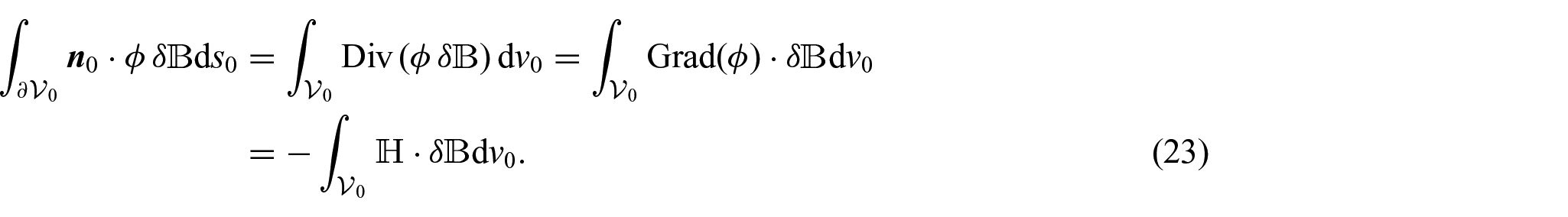
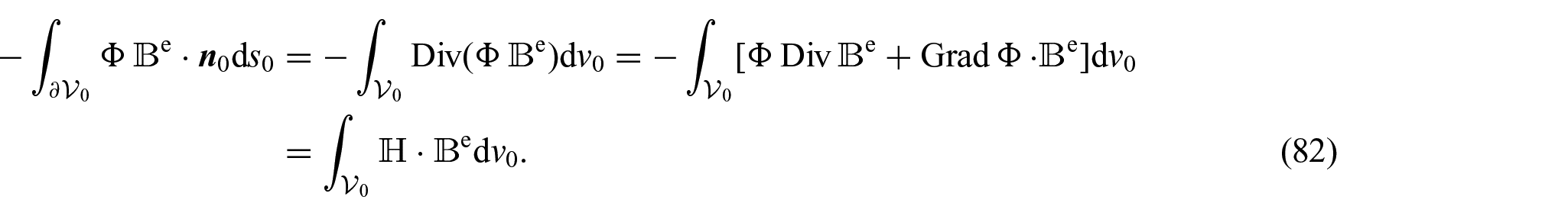
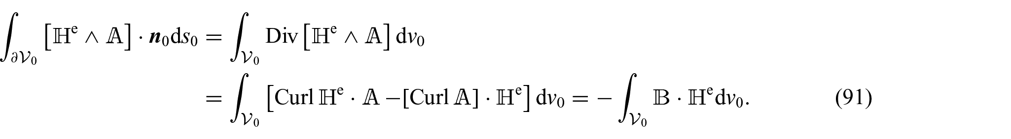
Apply the divergence theorem on the terms containing gradients of $\delta \chi$ to get

$$\begin{array}{c}\delta E_{\mathrm{II}}={\int }_{{\mathcal{B}}_0}(-(\mathrm{Div}({\rho }_0{\hat{\mathrm{\Omega }}}_{,\mathbf{F}}+{\overline{\mathbf{P}}}_m+{\stackrel{°}{\mathbf{P}}}_m-{\stackrel{⌣}{\mathbf{P}}}_m)+{\tilde{\mathit{f}}}^{\mathrm{e}}+{\rho }_{0}J{\mathbf{F}}^{-\mathrm{T}}(\mathrm{Gra}{\mathrm{d}}^{\mathrm{T}}{\mathbb{h}}^{\mathrm{e}}){\mathbf{F}}^{-\mathrm{T}}\overline{\mathbb{M}})·\delta \chi \hfill \\ +{\rho }_0({\hat{\mathrm{\Omega }}}_{,\overline{\mathbb{M}}}-J{\mathbf{F}}^{-1}{\mathbb{h}}^{\mathrm{e}}-J{\mathbf{F}}^{-1}{\mathbb{h}}^{\mathrm{s}})·\delta \overline{\mathbb{M}})\mathrm{d}{v}_0\hfill \\ +{\int }_{\partial {\mathcal{B}}_0}(({\rho }_0{\hat{\mathrm{\Omega }}}_{,\mathbf{F}}+{\overline{\mathbf{P}}}_m+{\stackrel{°}{\mathbf{P}}}_m-{\stackrel{⌣}{\mathbf{P}}}_m{)}_{-}{\mathit{n}}_0-({\stackrel{°}{\mathbf{P}}}_m-{\stackrel{⌣}{\mathbf{P}}}_m{)}_{+}{\mathit{n}}_0-{\tilde{\mathit{t}}}^{\mathrm{e}})·\delta \chi \mathrm{d}{s}_0\hfill \\ -{\int }_{\mathcal{B}{\prime }_0}\mathrm{Div}({\stackrel{°}{\mathbf{P}}}_m-{\stackrel{⌣}{\mathbf{P}}}_m)·\delta \chi \mathrm{d}{v}_0,\hfill \end{array}$$

(55)

where ${\overline{\mathbf{P}}}_m$ is defined by

$$\begin{array}{c}{\overline{\mathbf{P}}}_m:={\rho }_0(J{\mathbf{F}}^{-\mathrm{T}}\overline{\mathbb{M}}\otimes {\mathbb{h}}^{\mathrm{e}}-(J{\mathbf{F}}^{-\mathrm{T}}\overline{\mathbb{M}}·{\mathbb{h}}^{\mathrm{e}})\mathbf{I}){\mathbf{F}}^{-\mathrm{T}}\hfill \\ ={\rho }_0(J{\mathbf{F}}^{-\mathrm{T}}\overline{\mathbb{M}}\otimes {\mathbf{F}}^{-\mathrm{T}}{\mathbf{F}}^{\mathrm{T}}{\mathbb{h}}^{\mathrm{e}}-(J{\mathbf{F}}^{-1}{\mathbf{F}}^{-\mathrm{T}}\overline{\mathbb{M}}·{\mathbf{F}}^{\mathrm{T}}{\mathbb{h}}^{\mathrm{e}})\mathbf{I}){\mathbf{F}}^{-\mathrm{T}},\hfill \end{array}$$

(56)

and we have used the assumptions that $\chi$ and $\delta \chi$ are continuous across $\partial {\mathcal{B}}_0$ ; and ${\mathbb{h}}^{\mathrm{s}}\to 0$ as $\parallel \mathit{X}\parallel \to \infty$ . Note that

$$\begin{array}{c}{\stackrel{°}{\mathbf{P}}}_m+{\overline{\mathbf{P}}}_m=2{\stackrel{⌣}{\mathbf{P}}}_m+{\rho }_{0}J(-({\mathbf{C}}^{-1}\overline{\mathbb{M}}·{\mathbf{F}}^{\mathrm{T}}({\mathbb{h}}^{\mathrm{s}}+{\mathbb{h}}^e))\mathbf{I}+({\mathbf{F}}^{-\mathrm{T}}\overline{\mathbb{M}})\otimes {\mathbf{F}}^{-\mathrm{T}}{\mathbf{F}}^{\mathrm{T}}({\mathbb{h}}^{\mathrm{s}}+{\mathbb{h}}^e)\hfill \\ +({\mathbf{F}}^{-\mathrm{T}}{\mathbb{H}}^{\mathrm{s}})\otimes ({\mathbf{F}}^{-\mathrm{T}}\overline{\mathbb{M}})){\mathbf{F}}^{-\mathrm{T}}.\hfill \end{array}$$

(57)

In vacuum, $\overline{\mathbb{M}}=0$ , which leads to

$${\stackrel{°}{\mathbf{P}}}_m+{\overline{\mathbf{P}}}_m={\stackrel{°}{\mathbf{P}}}_m=2{\stackrel{⌣}{\mathbf{P}}}_m.$$

With the defining expression

$$\mathbf{P}={\rho }_0{\hat{\mathrm{\Omega }}}_{,\mathbf{F}}+{\overline{\mathbf{P}}}_m+{\stackrel{°}{\mathbf{P}}}_m-{\stackrel{⌣}{\mathbf{P}}}_m,$$

(58)

the tensor $\mathbf{P}$ can be identified as the total first Piola–Kirchhoff stress tensor and ${\mathbf{P}}^{★}=\mathbf{P}={\stackrel{⌣}{\mathbf{P}}}_m$ can be identified as the Maxwell stress tensor in vacuum.

Corresponding to the equilibrium condition of vanishing of the first variation $\delta E_{\mathrm{II}}$ of the potential energy $E_{\mathrm{II}}$ , using the classical methods in the calculus of variations [36], i.e.,

$$\delta E_{\mathrm{II}}(\chi ,\overline{\mathbb{M}})[\delta \chi ,\delta \overline{\mathbb{M}}]=0,$$

(59)

since the increment $\delta \overline{\mathbb{M}}$ is arbitrary, we arrive at the constitutive relation

$${\hat{\mathrm{\Omega }}}_{,\overline{\mathbb{M}}}=J{\mathbf{F}}^{-1}[{\mathbb{h}}^{\mathrm{s}}+{\mathbb{h}}^{\mathrm{e}}]=J{\mathbf{C}}^{-1}[{\mathbb{H}}^{\mathrm{s}}+{\mathbb{H}}^{\mathrm{e}}],$$

(60)

which is, remarkably, the same as equation (28).

Remark 10. In particular, inside the body $\mathbf{P}$ is given by (as $\mathbb{h}=J^{-1}\mathbf{F}{\hat{\mathrm{\Omega }}}_{,\overline{\mathbb{M}}}$ )

$$\begin{array}{c}\mathbf{P}={\rho }_0{\hat{\mathrm{\Omega }}}_{,\mathbf{F}}+{\rho }_{0}J(-({\mathbf{C}}^{-1}\overline{\mathbb{M}}·{\mathbf{F}}^{\mathrm{T}}\mathbb{h})\mathbf{I}+({\mathbf{F}}^{-\mathrm{T}}\overline{\mathbb{M}})\otimes {\mathbf{F}}^{-\mathrm{T}}{\mathbf{F}}^{\mathrm{T}}\mathbb{h}+{\mathbb{h}}^{\mathrm{s}}\otimes ({\mathbf{F}}^{-\mathrm{T}}\overline{\mathbb{M}})){\mathbf{F}}^{-\mathrm{T}}\hfill \\ +[{\mu }_{0}J{\mathbb{h}}^{\mathrm{s}}\otimes {\mathbb{h}}^{\mathrm{s}}-\frac{{\mu }_{0}J}{2}[{\mathbb{h}}^{\mathrm{s}}·{\mathbb{h}}^{\mathrm{s}}]\mathbf{I}]{\mathbf{F}}^{-\mathrm{T}}\hfill \\ ={\rho }_0{\hat{\mathrm{\Omega }}}_{,\mathbf{F}}+{\mu }_0{J}^{-1}[-\frac{J^2}{2}[{\mathbb{h}}^{\mathrm{s}}·{\mathbb{h}}^{\mathrm{s}}]\mathbf{I}+J^2{\mathbb{h}}^{\mathrm{s}}\otimes {\mathbb{h}}^{\mathrm{s}}]{\mathbf{F}}^{-\mathrm{T}}\hfill \\ +{\rho }_0[-(\overline{\mathbb{M}}·{\hat{\mathrm{\Omega }}}_{,\overline{\mathbb{M}}})\mathbf{I}+({\mathbf{F}}^{-\mathrm{T}}\overline{\mathbb{M}})\otimes \mathbf{F}{\hat{\mathrm{\Omega }}}_{,\overline{\mathbb{M}}}+J{\mathbb{h}}^{\mathrm{s}}\otimes ({\mathbf{F}}^{-\mathrm{T}}\overline{\mathbb{M}})]{\mathbf{F}}^{-\mathrm{T}},\hfill \end{array}$$

(61)

which differs from equation (30) by the following term:

$$\begin{array}{c}{\mathbf{P}}^N={\mu }_{0}J[-\frac{1}{2}[{\mathbb{h}}^{\mathrm{e}}·{\mathbb{h}}^{\mathrm{e}}]\mathbf{I}+{\mathbb{h}}^{\mathrm{e}}\otimes {\mathbb{h}}^{\mathrm{e}}]{\mathbf{F}}^{-\mathrm{T}}+{\mu }_{0}J[-[{\mathbb{h}}^{\mathrm{s}}·{\mathbb{h}}^{\mathrm{e}}]\mathbf{I}+{\mathbb{h}}^{\mathrm{s}}\otimes {\mathbb{h}}^{\mathrm{e}}+{\mathbb{h}}^{\mathrm{e}}\otimes {\mathbb{h}}^{\mathrm{s}}]{\mathbf{F}}^{-\mathrm{T}}\hfill \\ +{\rho }_{0}J{\mathbb{h}}^{\mathrm{e}}\otimes ({\mathbf{F}}^{-\mathrm{T}}\overline{\mathbb{M}}){\mathbf{F}}^{-\mathrm{T}}.\hfill \end{array}$$

(62)

With

$$\psi (a)=-\frac{1}{2}(a·a)\mathbf{I}+a\otimes a,$$

the first and second line in ${\mathbf{P}}^N$ can be written as $\psi ({\mathbb{h}}^{\mathrm{e}}+{\mathbb{h}}^{\mathrm{s}})-\psi ({\mathbb{h}}^{\mathrm{s}})$ . The difference between the two definitions of the stress tensor is not surprising. It is known that these could be different expressions, yet physically equivalent, as they depend on the formulation, see for example Hutter and van de Ven [39], who presented this aspect of the Maxwell stress tensor while analysing several formulations of electromagnetism in the theory of deformable media.

Since the increment $\delta \chi$ is arbitrary, we arrive at the following equations of equilibrium in magnetoelastostatics (for a system of a magnetoelastic body and its surrounding vacuum):

$$\mathrm{Div}\mathbf{P}+{\tilde{\mathit{f}}}^{\mathrm{e}}+{\rho }_{0}J{\mathbf{F}}^{-\mathrm{T}}[\mathrm{Gra}{\mathrm{d}}^{\mathrm{T}}{\mathbb{h}}^{\mathrm{e}}]{\mathbf{F}}^{-\mathrm{T}}\overline{\mathbb{M}}=0\mathrm{in}{\mathcal{B}}_0,$$

(63a)

$$\mathrm{Div}{\stackrel{⌣}{\mathbf{P}}}_m=0\mathrm{in}\mathcal{B}{\prime }_0$$

(63b)

$$[\mathbf{P}-{\stackrel{⌣}{\mathbf{P}}}_m]{\mathit{n}}_0={\tilde{\mathit{t}}}^{\mathrm{e}}\mathrm{on}p\partial {\mathcal{B}}_0.$$

(63c)

4.2. Perturbation of equilibrium equation at critical point

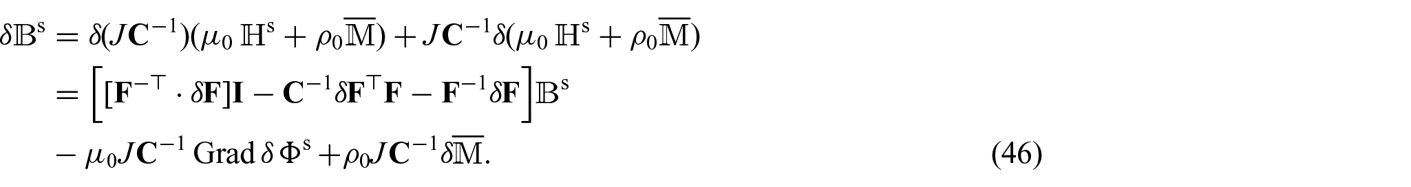
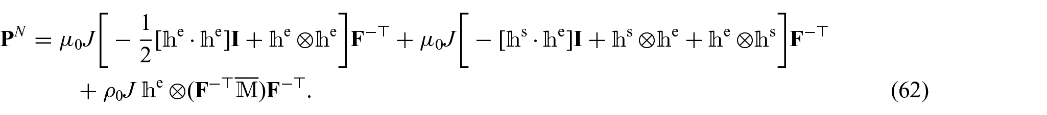
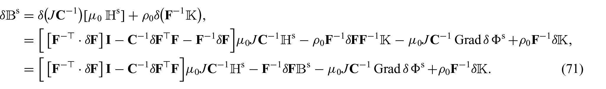
For the analysis of the critical point $(\chi ,\overline{\mathbb{M}})$ , the perturbations $\mathrm{\Delta }\chi$ and $\delta \overline{\mathbb{M}}$ in the equilibrium state need to satisfy certain incremental equations and boundary conditions. They are derived by a perturbation of equation (4.1) and are stated next. Recalling from equation (60) that ${\mathbb{h}}^{\mathrm{s}}=J^{-1}\mathbf{F}{\hat{\mathrm{\Omega }}}_{,\overline{\mathbb{M}}}-{\mathbb{h}}^{\mathrm{e}}$ , perturbation in the first Piola–Kirchhoff stress can be written using equation (61) as

$$\begin{array}{c}\mathrm{\Delta }\mathbf{P}={\rho }_0[{\hat{\mathrm{\Omega }}}_{,\mathbf{FF}}\mathrm{\Delta }\mathbf{F}+\frac{1}{2}[{\hat{\mathrm{\Omega }}}_{,\mathbf{F}\overline{\mathbb{M}}}+{\hat{\mathrm{\Omega }}}_{\mathbf{F}\overline{\mathbb{M}}}^{*}]\mathrm{\Delta }\overline{\mathbb{M}}]-{\mu }_0{J}^{-1}[{\mathbf{F}}^{-\mathrm{T}}·\mathrm{\Delta }\mathbf{F}][-\frac{J^2}{2}[{\mathbb{h}}^{\mathrm{s}}·{\mathbb{h}}^{\mathrm{s}}]\mathbf{I}+J^2{\mathbb{h}}^{\mathrm{s}}\otimes {\mathbb{h}}^{\mathrm{s}}]{\mathbf{F}}^{-\mathrm{T}}\hfill \\ +{\mu }_0{J}^{-1}[-J^2[[{\mathbf{F}}^{-\mathrm{T}}·\mathrm{\Delta }\mathbf{F}][{\mathbb{h}}^{\mathrm{s}}·{\mathbb{h}}^{\mathrm{s}}]+{\mathbb{h}}^{\mathrm{s}}·\mathrm{\Delta }{\mathbb{h}}^{\mathrm{s}}]\mathbf{I}+2J^2[{\mathbf{F}}^{-\mathrm{T}}·\mathrm{\Delta }\mathbf{F}]{\mathbb{h}}^{\mathrm{s}}\otimes {\mathbb{h}}^{\mathrm{s}}\hfill \\ +J^2[\mathrm{\Delta }{\mathbb{h}}^{\mathrm{s}}\otimes {\mathbb{h}}^{\mathrm{s}}+{\mathbb{h}}^{\mathrm{s}}\otimes \mathrm{\Delta }{\mathbb{h}}^{\mathrm{s}}]]{\mathbf{F}}^{-\mathrm{T}}\hfill \\ -{\mu }_0{J}^{-1}[-\frac{J^2}{2}[{\mathbb{h}}^{\mathrm{s}}·{\mathbb{h}}^{\mathrm{s}}]\mathbf{I}+J^2{\mathbb{h}}^{\mathrm{s}}\otimes {\mathbb{h}}^{\mathrm{s}}]{\mathbf{F}}^{-\mathrm{T}}[\mathrm{\Delta }\mathbf{F}{]}^{\mathrm{T}}{\mathbf{F}}^{-\mathrm{T}}\hfill \\ +{\rho }_0[-[\mathrm{\Delta }\overline{\mathbb{M}}·{\hat{\mathrm{\Omega }}}_{,\overline{\mathbb{M}}}+\overline{\mathbb{M}}·[\frac{1}{2}[{\hat{\mathrm{\Omega }}}_{,\overline{\mathbb{M}}\mathbf{F}}+{\hat{\mathrm{\Omega }}}_{\overline{\mathbb{M}}\mathbf{F}}^{*}]\mathrm{\Delta }\mathbf{F}+{\hat{\mathrm{\Omega }}}_{,\overline{\mathbb{M}}\overline{\mathbb{M}}}\mathrm{\Delta }\overline{\mathbb{M}}]]\mathbf{I}\hfill \\ +[-{\mathbf{F}}^{-\mathrm{T}}\mathrm{\Delta }\mathbf{F}{\mathbf{F}}^{-\mathrm{T}}\overline{\mathbb{M}}+{\mathbf{F}}^{-\mathrm{T}}\mathrm{\Delta }\overline{\mathbb{M}}]\otimes \mathbf{F}{\hat{\mathrm{\Omega }}}_{,\overline{\mathbb{M}}}\hfill \\ +{\mathbf{F}}^{-\mathrm{T}}\overline{\mathbb{M}}\otimes [\mathrm{\Delta }\mathbf{F}{\hat{\mathrm{\Omega }}}_{,\overline{\mathbb{M}}}+\frac{1}{2}\mathbf{F}[{\hat{\mathrm{\Omega }}}_{,\overline{\mathbb{M}}\mathbf{F}}+{\hat{\mathrm{\Omega }}}_{\overline{\mathbb{M}}\mathbf{F}}^{*}]\mathrm{\Delta }\mathbf{F}+\mathbf{F}{\hat{\mathrm{\Omega }}}_{,\overline{\mathbb{M}}\overline{\mathbb{M}}}\mathrm{\Delta }\overline{\mathbb{M}}]\hfill \\ +[J[{\mathbf{F}}^{-\mathrm{T}}·\mathrm{\Delta }\mathbf{F}]{\mathbb{h}}^{\mathrm{s}}+J\mathrm{\Delta }{\mathbb{h}}^{\mathrm{s}}]\otimes [{\mathbf{F}}^{-\mathrm{T}}\overline{\mathbb{M}}]+J{\mathbb{h}}^{\mathrm{s}}\otimes [{\mathbf{F}}^{-\mathrm{T}}\mathrm{\Delta }\overline{\mathbb{M}}-{\mathbf{F}}^{-\mathrm{T}}{[\mathrm{\Delta }\mathbf{F}]}^{\mathrm{T}}{\mathbf{F}}^{-\mathrm{T}}]]{\mathbf{F}}^{-\mathrm{T}}\hfill \\ -{\rho }_0[-(\overline{\mathbb{M}}·{\hat{\mathrm{\Omega }}}_{,\overline{\mathbb{M}}})\mathbf{I}+({\mathbf{F}}^{-\mathrm{T}}\overline{\mathbb{M}})\otimes \mathbf{F}{\hat{\mathrm{\Omega }}}_{,\overline{\mathbb{M}}}+J{\mathbb{h}}^{\mathrm{s}}\otimes ({\mathbf{F}}^{-\mathrm{T}}\overline{\mathbb{M}})]{\mathbf{F}}^{-\mathrm{T}}[\mathrm{\Delta }\mathbf{F}{]}^{\mathrm{T}}{\mathbf{F}}^{-\mathrm{T}},\hfill \end{array}$$

(64)

where we can obtain the expression for $\mathrm{\Delta }{\mathbb{h}}^{\mathrm{s}}$ from equation (60) as

$$\mathrm{\Delta }{\mathbb{h}}^{\mathrm{s}}=J^{-1}\mathbf{F}[{\hat{\mathrm{\Omega }}}_{,\overline{\mathbb{M}}\mathbf{F}}\mathrm{\Delta }\mathbf{F}+{\hat{\mathrm{\Omega }}}_{,\overline{\mathbb{M}}\overline{\mathbb{M}}}\mathrm{\Delta }\overline{\mathbb{M}}]-J^{-1}[{\mathbf{F}}^{-\mathrm{T}}·\mathrm{\Delta }\mathbf{F}]\mathbf{F}{\hat{\mathrm{\Omega }}}_{,\overline{\mathbb{M}}}+J^{-1}\mathrm{\Delta }\mathbf{F}{\hat{\mathrm{\Omega }}}_{,\overline{\mathbb{M}}}.$$

(65)

We have also introduced two second-order tensors ${\hat{\mathrm{\Omega }}}_{\overline{\mathbb{M}}\mathbf{F}}^{*}$ and ${\hat{\mathrm{\Omega }}}_{\mathbf{F}\overline{\mathbb{M}}}^{*}$ with the property

$$[{\hat{\mathrm{\Omega }}}_{\overline{\mathbb{M}}\mathbf{F}}^{*}\mathbf{U}]\mathit{u}=[{\hat{\mathrm{\Omega }}}_{,\mathbf{F}\overline{\mathbb{M}}}\mathit{u}]·\mathbf{U},[{\hat{\mathrm{\Omega }}}_{\mathbf{F}\overline{\mathbb{M}}}^{*}\mathit{u}]·\mathbf{U}=[{\hat{\mathrm{\Omega }}}_{,\overline{\mathbb{M}}\mathbf{F}}\mathbf{U}]·\mathit{u}.$$

(66)

for arbitrary vector $\mathit{u}$ and arbitrary second-order tensor $\mathbf{U}$ . The expression for $\mathrm{\Delta }{\stackrel{⌣}{\mathbf{P}}}_m$ is obtained from equation (45) as

$$\begin{array}{c}\mathrm{\Delta }{\stackrel{⌣}{\mathbf{P}}}_m={\mu }_{0}J[{\mathbf{F}}^{-\mathrm{T}}·\mathrm{\Delta }\mathbf{F}][{\mathbb{h}}^{\mathrm{s}}\otimes {\mathbb{h}}^{\mathrm{s}}-\frac{1}{2}[{\mathbb{h}}^{\mathrm{s}}·{\mathbb{h}}^{\mathrm{s}}]\mathbf{I}]{\mathbf{F}}^{-\mathrm{T}}+{\mu }_{0}J[{\mathbb{h}}^{\mathrm{s}}\otimes \mathrm{\Delta }{\mathbb{h}}^{\mathrm{s}}+\mathrm{\Delta }{\mathbb{h}}^{\mathrm{s}}\otimes {\mathbb{h}}^{\mathrm{s}}-[{\mathbb{h}}^{\mathrm{s}}·\mathrm{\Delta }{\mathbb{h}}^{\mathrm{s}}]\mathbf{I}]{\mathbf{F}}^{-\mathrm{T}}\hfill \\ -{\mu }_{0}J[{\mathbb{h}}^{\mathrm{s}}\otimes {\mathbb{h}}^{\mathrm{s}}-\frac{1}{2}[{\mathbb{h}}^{\mathrm{s}}·{\mathbb{h}}^{\mathrm{s}}]\mathbf{I}]{\mathbf{F}}^{-\mathrm{T}}[\mathrm{\Delta }\mathbf{F}{]}^{\mathrm{T}}{\mathbf{F}}^{-\mathrm{T}}.\hfill \end{array}$$

(67)

Finally, this leads to the following partial differential equations and boundary conditions:

$$\begin{array}{c}\mathrm{Div}\mathrm{\Delta }\mathbf{P}+{\rho }_{0}J{\mathbf{F}}^{-\mathrm{T}}[\mathrm{Gra}{\mathrm{d}}^{\mathrm{T}}{\mathbb{h}}^{\mathrm{e}}]{\mathbf{F}}^{-\mathrm{T}}\mathrm{\Delta }\overline{\mathbb{M}}\hfill \\ +{\rho }_{0}J[{\mathbf{F}}^{-\mathrm{T}}·\mathrm{\Delta }\mathbf{F}]{\mathbf{F}}^{-\mathrm{T}}[\mathrm{Gra}{\mathrm{d}}^{\mathrm{T}}{\mathbb{h}}^{\mathrm{e}}]{\mathbf{F}}^{-\mathrm{T}}\overline{\mathbb{M}}\hfill \\ -{\rho }_{0}J{\mathbf{F}}^{-\mathrm{T}}[\mathrm{\Delta }\mathbf{F}{]}^{\mathrm{T}}{\mathbf{F}}^{-\mathrm{T}}[\mathrm{Gra}{\mathrm{d}}^{\mathrm{T}}{\mathbb{h}}^{\mathrm{e}}]{\mathbf{F}}^{-\mathrm{T}}\overline{\mathbb{M}}\hfill \\ -{\rho }_{0}J{\mathbf{F}}^{-\mathrm{T}}[\mathrm{Gra}{\mathrm{d}}^{\mathrm{T}}{\mathbb{h}}^{\mathrm{e}}]{\mathbf{F}}^{-\mathrm{T}}[\mathrm{\Delta }\mathbf{F}{]}^{\mathrm{T}}{\mathbf{F}}^{-\mathrm{T}}\overline{\mathbb{M}}=0\mathrm{in}{\mathcal{B}}_0,\hfill \end{array}$$

(68a)

$$\mathrm{Div}\mathrm{\Delta }{\stackrel{⌣}{\mathbf{P}}}_m=0\mathrm{in}\mathcal{B}{\prime }_0$$

(68b)

$$[\mathrm{\Delta }\mathbf{P}-\mathrm{\Delta }{\stackrel{⌣}{\mathbf{P}}}_m]{\mathit{n}}_0=0\mathrm{on}\partial {\mathcal{B}}_0.$$

(68c)

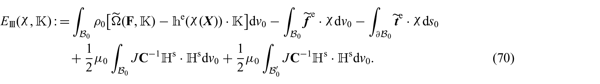
5. Third formulation based on magnetisation

In the backdrop of the two formulations provided thus far based on the magnetisation, we investigate in this section the expressions provided by [13], which also assume that the stored energy density depends on the magnetisation as the additional field besides the deformation gradient. Following [13], in this case, the magnetisation per unit mass pulled back to the reference configuration (recall equation (9)), i.e.,

$$\mathbb{K}(\mathit{X}):=\overline{\mathbb{m}}(\mathit{x})=J(\mathit{X}){\mathbf{F}}^{-\mathrm{T}}(\mathit{X})\overline{\mathbb{M}}(\mathit{X}),\mathit{X}\in {\mathcal{B}}_0,$$

(69)

is itself treated as a material field. In particular, note that the direction of the referential vector field $\mathbb{K}$ on ${\mathcal{B}}_0$ is the same as that of the spatial vector field $\overline{\mathbb{m}}$ on $\mathcal{B}$ , while it differs from the choice of the referential field $\overline{\mathbb{M}}$ , owing to the presence of the cofactor map for $\mathbf{F}$ (Nanson’s relation). The total potential energy of the system is written as

$$\begin{array}{c}{E}_{\mathrm{III}}(\chi ,\mathbb{K}):={\int }_{{\mathcal{B}}_0}{\rho }_0[\tilde{\mathrm{\Omega }}(\mathbf{F},\mathbb{K})-{\mathbb{h}}^{\mathrm{e}}(\chi (\mathit{X}))·\mathbb{K}]\mathrm{d}{v}_0-{\int }_{{\mathcal{B}}_0}{\tilde{\mathit{f}}}^{\mathrm{e}}·\chi \mathrm{d}{v}_0-{\int }_{\partial {\mathcal{B}}_0}{\tilde{\mathit{t}}}^{\mathrm{e}}·\chi \mathrm{d}{s}_0\hfill \\ +\frac{1}{2}{\mu }_0{\int }_{{\mathcal{B}}_0}J{\mathbf{C}}^{-1}{\mathbb{H}}^{\mathrm{s}}·{\mathbb{H}}^{\mathrm{s}}\mathrm{d}{v}_0+\frac{1}{2}{\mu }_0{\int }_{\mathcal{B}{\prime }_0}J{\mathbf{C}}^{-1}{\mathbb{H}}^{\mathrm{s}}·{\mathbb{H}}^{\mathrm{s}}\mathrm{d}{v}_0.\hfill \end{array}$$

(70)

Here, $\widetilde{{\mathit{f}}^{\mathrm{e}}}$ represents the body force (per unit volume) and ${\tilde{\mathit{t}}}^{\mathrm{e}}$ denotes the mechanical traction. In contrast to equation (37), the term corresponding to the Zeeman energy is written differently. Note from equation (17) that $J^{-1}\mathbf{F}{\mathbb{B}}^{\mathrm{s}}={\mu }_0{\mathbf{F}}^{-\mathrm{T}}{\mathbb{H}}^{\mathrm{s}}+\rho \mathbb{K},$ i.e., ${\mathbb{B}}^{\mathrm{s}}={\mu }_{0}J{\mathbf{C}}^{-1}{\mathbb{H}}^{\mathrm{s}}+{\rho }_0{\mathbf{F}}^{-1}\mathbb{K}$ , so that

$$\begin{array}{c}\delta {\mathbb{B}}^{\mathrm{s}}=\delta (J{\mathbf{C}}^{-1})[{\mu }_0{\mathbb{H}}^{\mathrm{s}}]+{\rho }_0\delta ({\mathbf{F}}^{-1}\mathbb{K}),\hfill \\ =[[{\mathbf{F}}^{-\mathrm{T}}·\delta \mathbf{F}]\mathbf{I}-{\mathbf{C}}^{-1}\delta {\mathbf{F}}^{\mathrm{T}}\mathbf{F}-{\mathbf{F}}^{-1}\delta \mathbf{F}]{\mu }_{0}J{\mathbf{C}}^{-1}{\mathbb{H}}^{\mathrm{s}}-{\rho }_0{\mathbf{F}}^{-1}\delta \mathbf{F}{\mathbf{F}}^{-1}\mathbb{K}-{\mu }_{0}J{\mathbf{C}}^{-1}\mathrm{Grad}\delta {\mathrm{\Phi }}^{\mathrm{s}}+{\rho }_0{\mathbf{F}}^{-1}\delta \mathbb{K},\hfill \\ =[[{\mathbf{F}}^{-\mathrm{T}}·\delta \mathbf{F}]\mathbf{I}-{\mathbf{C}}^{-1}\delta {\mathbf{F}}^{\mathrm{T}}\mathbf{F}]{\mu }_{0}J{\mathbf{C}}^{-1}{\mathbb{H}}^{\mathrm{s}}-{\mathbf{F}}^{-1}\delta \mathbf{F}{\mathbb{B}}^{\mathrm{s}}-{\mu }_{0}J{\mathbf{C}}^{-1}\mathrm{Grad}\delta {\mathrm{\Phi }}^{\mathrm{s}}+{\rho }_0{\mathbf{F}}^{-1}\delta \mathbb{K}.\hfill \end{array}$$

(71)

Using this relation, we can rewrite the following integral, which occurs in the first variation of potential energy:

$$-{\mu }_0{\int }_{{\mathcal{B}}_0}J{\mathbf{C}}^{-1}{\mathbb{H}}^{\mathrm{s}}·\delta {\mathbb{H}}^{\mathrm{s}}\mathrm{d}{v}_0={\int }_{{\mathcal{B}}_0}-{\tilde{\mathbf{P}}}_m·\delta \mathbf{F}\mathrm{d}{v}_0+{\int }_{{\mathcal{B}}_0}{\mathbb{H}}^{\mathrm{s}}·({\rho }_0{\mathbf{F}}^{-1}\delta \mathbb{K}-\delta {\mathbb{B}}^{\mathrm{s}})\mathrm{d}{v}_0,$$

(72)

where the integrand of the first term on the right-hand side, i.e., $-{\tilde{\mathbf{P}}}_m·\delta \mathbf{F}$ , can be expanded as

$$\begin{array}{c}-{\tilde{\mathbf{P}}}_m·\delta \mathbf{F}={\mu }_{0}J({\mathbf{F}}^{-\mathrm{T}}·\delta \mathbf{F}){\mathbf{C}}^{-1}{\mathbb{H}}^{\mathrm{s}}·{\mathbb{H}}^{\mathrm{s}}-{\mu }_{0}J{\mathbf{C}}^{-1}\delta {\mathbf{F}}^{\mathrm{T}}\mathbf{F}{\mathbf{C}}^{-1}{\mathbb{H}}^{\mathrm{s}}·{\mathbb{H}}^{\mathrm{s}}-{\mathbf{F}}^{-\mathrm{T}}{\mathbb{H}}^{\mathrm{s}}\otimes {\mathbb{B}}^{\mathrm{s}}·\delta \mathbf{F}\hfill \\ =(-2{\stackrel{⌣}{\mathbf{P}}}_m-{\rho }_0{\mathbb{h}}^{\mathrm{s}}\otimes \mathbb{K}{\mathbf{F}}^{-\mathrm{T}})·\delta \mathbf{F}.\hfill \end{array}$$

(73)

Thus,

$${\tilde{\mathbf{P}}}_m-{\stackrel{⌣}{\mathbf{P}}}_m={\stackrel{⌣}{\mathbf{P}}}_m+{\rho }_0{\mathbb{h}}^{\mathrm{s}}\otimes \mathbb{K}{\mathbf{F}}^{-\mathrm{T}}={\stackrel{⌣}{\mathbf{P}}}_m+J{\mathbb{h}}^{\mathrm{s}}\otimes \mathbb{m}{\mathbf{F}}^{-\mathrm{T}}.$$

(74)

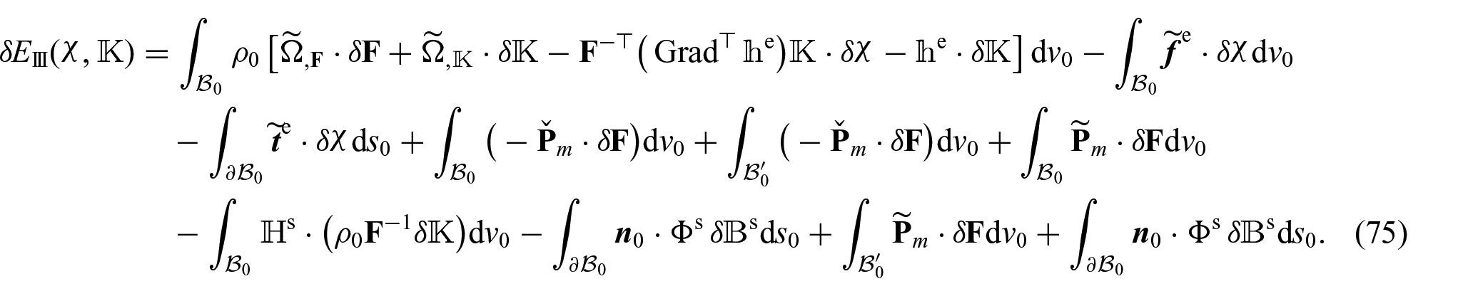
From equation (44), we already know a part of the expression of the first variation of the stray field energy term. Therefore, we write the first variation of the potential energy (equation (70)) as

$$\begin{array}{l}\delta E_{\mathrm{III}}(\chi ,\mathbb{K})={\int }_{{ℬ}_0}{\rho }_0\left[{\tilde{\mathrm{\Omega }}}_{,\mathbf{F}}\cdot \delta \mathbf{F}+{\tilde{\mathrm{\Omega }}}_{,\mathbb{K}}\cdot \delta \mathbb{K}-{\mathbf{F}}^{-{\rm T}}({\mathrm{Grad}}^{{\rm T}}{\mathrm{h}}^{\mathrm{e}})\mathbb{K}\cdot \delta \chi -{\mathrm{h}}^{\mathrm{e}}\cdot \delta \mathbb{K}\right]\mathrm{d}{v}_0-{\int }_{{ℬ}_0}{\tilde{\mathit{f}}}^{\mathrm{e}}\cdot \delta \chi \mathrm{d}{v}_0\\ -{\int }_{\partial {ℬ}_0}{\tilde{\mathit{t}}}^{\mathrm{e}}\cdot \delta \chi \mathrm{d}{s}_0+{\int }_{{ℬ}_0}(-{\stackrel{⌣}{\mathbf{P}}}_m\cdot \delta \mathbf{F})\mathrm{d}{v}_0+{\int }_{{ℬ\prime }_0}(-{\stackrel{⌣}{\mathbf{P}}}_m\cdot \delta \mathbf{F})\mathrm{d}{v}_0+{\int }_{{ℬ}_0}{\tilde{\mathbf{P}}}_m\cdot \delta \mathbf{F}\mathrm{d}{v}_0\\ -{\int }_{{ℬ}_0}{\mathbb{H}}^{\mathrm{s}}\cdot ({\rho }_0{\mathbf{F}}^{-1}\delta \mathbb{K})\mathrm{d}{v}_0-{\int }_{\partial {ℬ}_0}{\mathit{n}}_0\cdot {\mathrm{\Phi }}^{\mathrm{s}}\delta {\mathbb{B}}^{\mathrm{s}}\mathrm{d}{s}_0+{\int }_{{ℬ}_{0^{\prime }}}{\tilde{\mathbf{P}}}_m\cdot \delta \mathbf{F}\mathrm{d}{v}_0+{\int }_{\partial {ℬ}_0}{\mathit{n}}_0\cdot {\mathrm{\Phi }}^{\mathrm{s}}\delta {\mathbb{B}}^{\mathrm{s}}\mathrm{d}{s}_0.\end{array}$$

(75)

On applying the divergence theorem on the terms containing the gradient of $\delta \chi$ , we get

$$\begin{array}{l}\delta E_{\mathrm{III}}={\int }_{{ℬ}_0}\left(-\left[\mathrm{Div}({\rho }_0{\tilde{\mathrm{\Omega }}}_{,\mathbf{F}}+{\tilde{\mathbf{P}}}_m-{\stackrel{⌣}{\mathbf{P}}}_m)+{\tilde{\mathit{f}}}^{\mathrm{e}}+{\rho }_0{\mathbf{F}}^{-{\rm T}}({\mathrm{Grad}}^{{\rm T}}{\mathrm{h}}^{\mathrm{e}})\mathbb{K}\right]\cdot \delta \chi +{\rho }_0[{\tilde{\mathrm{\Omega }}}_{,\mathbb{K}}-{\mathrm{h}}^{\mathrm{e}}-{\mathrm{h}}^{\mathrm{s}}]\cdot \delta \mathbb{K}\right)\mathrm{d}{v}_0\\ +{\int }_{\partial {ℬ}_0}\left({({\rho }_0{\tilde{\mathrm{\Omega }}}_{,\mathbf{F}}+{\tilde{\mathbf{P}}}_m-{\stackrel{⌣}{\mathbf{P}}}_m)}_{-}{\mathit{n}}_0-{({\tilde{\mathbf{P}}}_m-{\stackrel{⌣}{\mathbf{P}}}_m)}_{+}{\mathit{n}}_0-{\tilde{\mathit{t}}}^{\mathrm{e}}\right)\cdot \delta \chi \mathrm{d}{s}_0-{\int }_{{ℬ\prime }_0}\mathrm{Div}({\tilde{\mathbf{P}}}_m-{\stackrel{⌣}{\mathbf{P}}}_m)\cdot \delta \chi \mathrm{d}{v}_0.\end{array}$$

(76)

Since the increments $\delta \chi$ and $\delta \mathbb{K}$ are arbitrary, we arrive at the following Euler–Lagrange equations for this variational problem:

$$\mathrm{Div}\mathbf{P}+{\tilde{\mathit{f}}}^{\mathrm{e}}+{\rho }_0{\mathbf{F}}^{-\mathrm{T}}(\mathrm{Gra}{\mathrm{d}}^{\mathrm{T}}{\mathbb{h}}^{\mathrm{e}})\mathbb{K}=0\mathrm{in}{\mathcal{B}}_0,$$

(77a)

$$\left[\left[\mathbf{P}\right]\right]{\mathit{n}}_0+{\tilde{\mathit{t}}}^{\mathrm{e}}=0\mathrm{on}\partial {\mathcal{B}}_0,$$

(77b)

$$\mathrm{Div}\mathbf{P}=0\mathrm{in}\mathcal{B}{\prime }_0$$

(77c)

$$\mathbb{h}={\tilde{\mathrm{\Omega }}}_{,\mathbb{K}}\mathrm{in}{\mathcal{B}}_0,$$

(77d)

where we have recognised the total first Piola–Kirchhoff stress tensor in the body and in vacuum as

$$\mathbf{P}={\rho }_0{\tilde{\mathrm{\Omega }}}_{,\mathbf{F}}+{\tilde{\mathbf{P}}}_m-{\stackrel{⌣}{\mathbf{P}}}_m\mathrm{in}{\mathcal{B}}_0,$$

(78a)

$$\mathbf{P}={\tilde{\mathbf{P}}}_m-{\stackrel{⌣}{\mathbf{P}}}_m\mathrm{in}\mathcal{B}{\prime }_0.$$

(78b)

Remark 11. From equations (45) and (74) (recall Remark 4), we can write the total Cauchy stress on $\mathcal{B}$ as

$$\sigma =J^{-1}\mathbf{P}{\mathbf{F}}^{\mathrm{T}}=\rho {\tilde{\mathrm{\Omega }}}_{,\mathbf{F}}{\mathbf{F}}^{\mathrm{T}}+{\mathbb{h}}^{\mathrm{s}}\otimes {\mathbb{b}}^{\mathrm{s}}-\frac{1}{2}{\mu }_0({\mathbb{h}}^{\mathrm{s}}·{\mathbb{h}}^{\mathrm{s}})\mathbf{I}.$$

(79)

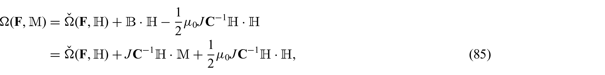
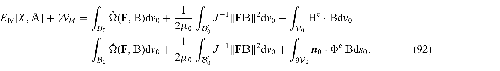
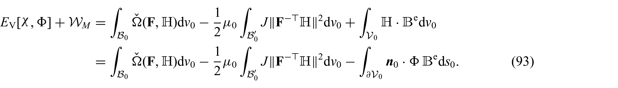
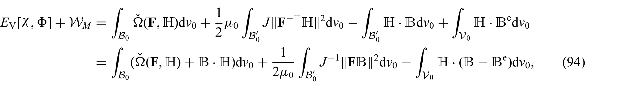
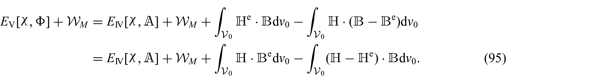
6. Correspondence between variational principles

Thus far, we have presented three different magnetisation-based formulations, where the difference between these variational principles occurs as a result of the choice of particular magnetisation field. In addition to these, we also present two other formulations in Appendices C and D, where, in place of the magnetisation field, the stored energy density depends on $\mathbb{B}$ and $\mathbb{H}$ , respectively. Since the mechanical work terms involving the body force and the surface traction are the same in all these formulations (in the referential description), i.e.,

$${\mathcal{W}}_M:=-{\int }_{{\mathcal{B}}_0}{\tilde{\mathit{f}}}^{\mathrm{e}}·\chi \mathrm{d}{v}_0-{\int }_{\partial {\mathcal{B}}_0}{\tilde{\mathit{t}}}^{\mathrm{e}}·\chi \mathrm{d}{s}_0,$$

(which also equals its spatial description $-{\int }_{\mathcal{B}}\rho {\mathit{f}}^{\mathrm{e}}·\chi \mathrm{d}v-{\int }_{\partial \mathcal{B}}{\mathit{t}}^{\mathrm{e}}·\chi \mathrm{d}s$ ), we sometimes compare only the remaining terms. Using the constitutive relation (equation (11)) and the fact that $\mathbb{M}$ vanishes outside the body ${\mathcal{B}}_0$ , we get

$$\frac{1}{2}{\mu }_0{\int }_{{\mathcal{V}}_0}J\parallel {\mathbf{F}}^{-\mathrm{T}}\mathbb{H}{\parallel }^2\mathrm{d}{v}_0-{\int }_{{\mathcal{V}}_0}\mathbb{H}·\mathbb{B}\mathrm{d}{v}_0=-\frac{1}{2}{\mu }_0{\int }_{{\mathcal{V}}_0}J\parallel {\mathbf{F}}^{-\mathrm{T}}\mathbb{H}{\parallel }^2\mathrm{d}{v}_0-{\int }_{{\mathcal{B}}_0}J{\mathbf{C}}^{-1}\mathbb{M}·\mathbb{H}\mathrm{d}{v}_0.$$

(80)

In a similar manner, we find that

$$\frac{1}{2}{\mu }_0{\int }_{\mathcal{B}{\prime }_0}J\parallel {\mathbf{F}}^{-\mathrm{T}}\mathbb{H}{\parallel }^2\mathrm{d}{v}_0-{\int }_{\mathcal{B}{\prime }_0}\mathbb{H}·\mathbb{B}\mathrm{d}{v}_0=-\frac{1}{2}{\mu }_0{\int }_{\mathcal{B}{\prime }_0}J\parallel {\mathbf{F}}^{-\mathrm{T}}\mathbb{H}{\parallel }^2\mathrm{d}{v}_0.$$

(81)

At this point, it is useful to recall Remark 2. Using equations (7) and (8),

$$\begin{array}{c}-{\int }_{\partial {\mathcal{V}}_0}\mathrm{\Phi }{\mathbb{B}}^{\mathrm{e}}·{\mathit{n}}_0\mathrm{d}{s}_0=-{\int }_{{\mathcal{V}}_0}\mathrm{Div}(\mathrm{\Phi }{\mathbb{B}}^{\mathrm{e}})\mathrm{d}{v}_0=-{\int }_{{\mathcal{V}}_0}[\mathrm{\Phi }\mathrm{Div}{\mathbb{B}}^{\mathrm{e}}+\mathrm{Grad}\mathrm{\Phi }·{\mathbb{B}}^{\mathrm{e}}]\mathrm{d}{v}_0\hfill \\ ={\int }_{{\mathcal{V}}_0}\mathbb{H}·{\mathbb{B}}^{\mathrm{e}}\mathrm{d}{v}_0.\hfill \end{array}$$

(82)

In general, we have

$$\begin{array}{c}{\int }_{{\mathcal{V}}_0}\mathbb{H}·\mathbb{B}\mathrm{d}{v}_0=-{\int }_{\partial {\mathcal{V}}_0}{\mathit{n}}_0·\mathrm{\Phi }\mathbb{B}\mathrm{d}{s}_0,\hfill \\ {\int }_{{\mathcal{V}}_0}\mathbb{H}·{\mathbb{B}}^{\mathrm{e}}\mathrm{d}{v}_0=-{\int }_{\partial {\mathcal{V}}_0}{\mathit{n}}_0·\mathrm{\Phi }{\mathbb{B}}^{\mathrm{e}}\mathrm{d}{s}_0,\hfill \\ {\int }_{{\mathcal{V}}_0}{\mathbb{H}}^{\mathrm{e}}·\mathbb{B}\mathrm{d}{v}_0=-{\int }_{\partial {\mathcal{V}}_0}{\mathit{n}}_0·{\mathrm{\Phi }}^{\mathrm{e}}\mathbb{B}\mathrm{d}{s}_0.\hfill \end{array}$$

(83)

Also, these relations can be rewritten further, for example,

$${\int }_{{\mathcal{V}}_0}\mathbb{H}·{\mathbb{B}}^{\mathrm{e}}\mathrm{d}{v}_0=-{\int }_{\partial {\mathcal{V}}_0}{\mathit{n}}_0·\mathrm{\Phi }{\mathbb{B}}^{\mathrm{e}}\mathrm{d}{s}_0=-{\mu }_0{\int }_{\partial {\mathcal{V}}_0}{\mathit{n}}_0·\mathrm{\Phi }J{\mathbf{C}}^{-1}{\mathbb{H}}^{\mathrm{e}}\mathrm{d}{s}_0.$$

6.1. Potential energy functionals based on $\mathbb{M}$ , $\mathbb{B}$ and $\mathbb{H}$

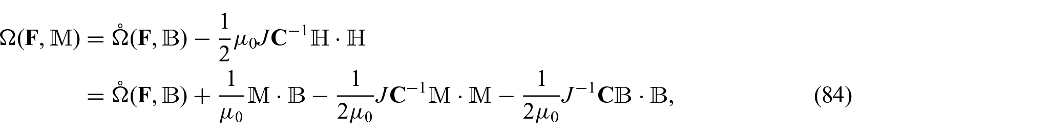
The variational formulations based on $\mathbb{B}$ and $\mathbb{H}$ can be related by applying a Legendre-type transform on the energy functions $\stackrel{°}{\mathrm{\Omega }}$ and $\stackrel{⌣}{\mathrm{\Omega }}$ as $\stackrel{°}{\mathrm{\Omega }}(\mathbf{F},\mathbb{B})=\stackrel{⌣}{\mathrm{\Omega }}(\mathbf{F},\mathbb{H})+\mathbb{B}·\mathbb{H}$ [14]. Moreover, we note that the three variational formulations based on $\mathbb{M}$ , $\mathbb{B}$ and $\mathbb{H}$ can be mutually related by a set of Legendre-type transforms on the stored energy density functions $\mathrm{\Omega },\stackrel{°}{\mathrm{\Omega }}$ and $\stackrel{⌣}{\mathrm{\Omega }}$ , respectively, so that

$$\begin{array}{c}\mathrm{\Omega }(\mathbf{F},\mathbb{M})=\stackrel{°}{\mathrm{\Omega }}(\mathbf{F},\mathbb{B})-\frac{1}{2}{\mu }_{0}J{\mathbf{C}}^{-1}\mathbb{H}·\mathbb{H}\hfill \\ =\stackrel{°}{\mathrm{\Omega }}(\mathbf{F},\mathbb{B})+\frac{1}{{\mu }_0}\mathbb{M}·\mathbb{B}-\frac{1}{2{\mu }_0}J{\mathbf{C}}^{-1}\mathbb{M}·\mathbb{M}-\frac{1}{2{\mu }_0}{J}^{-1}\mathbf{C}\mathbb{B}·\mathbb{B},\hfill \end{array}$$

(84)

$$\begin{array}{c}\mathrm{\Omega }(\mathbf{F},\mathbb{M})=\stackrel{⌣}{\mathrm{\Omega }}(\mathbf{F},\mathbb{H})+\mathbb{B}·\mathbb{H}-\frac{1}{2}{\mu }_{0}J{\mathbf{C}}^{-1}\mathbb{H}·\mathbb{H}\hfill \\ =\stackrel{⌣}{\mathrm{\Omega }}(\mathbf{F},\mathbb{H})+J{\mathbf{C}}^{-1}\mathbb{H}·\mathbb{M}+\frac{1}{2}{\mu }_{0}J{\mathbf{C}}^{-1}\mathbb{H}·\mathbb{H},\hfill \end{array}$$

(85)

$$\stackrel{°}{\mathrm{\Omega }}(\mathbf{F},\mathbb{B})=\stackrel{⌣}{\mathrm{\Omega }}(\mathbf{F},\mathbb{H})+\mathbb{B}·\mathbb{H}.$$

(86)

By a direct calculation, it can be verified that these relations result in the magnetic constitutive relations (equations (126), (143) and (28)); in particular,

$${\stackrel{°}{\mathrm{\Omega }}}_{,\mathbb{B}}=\mathbb{H},{\stackrel{⌣}{\mathrm{\Omega }}}_{,\mathbb{H}}=-\mathbb{B},{\mathrm{\Omega }}_{,\mathbb{M}}=J{\mathbf{C}}^{-1}\mathbb{H}\mathrm{in}{\mathcal{B}}_0.$$

As such, these relations lead to different convexity properties for $\stackrel{°}{\mathrm{\Omega }}(\mathbf{F},\mathbb{B})$ , $\stackrel{⌣}{\mathrm{\Omega }}(\mathbf{F},\mathbb{H})$ and $\mathrm{\Omega }(\mathbf{F},\mathbb{M})$ in general.

As a consequence, it is natural to establish the relationship between the three variational formulations based on $\mathbb{B}$ , $\mathbb{H}$ and $\mathbb{M}$ . Recall that the total potential energy (equation (18)) is a functional of the deformation $\chi$ (equations (1) (2)) and the referential magnetisation $\mathbb{M}$ (equation (12)). Indeed, the variational formulation (equation (18)) can be expressed as

$$\begin{array}{c}{E}_{\mathrm{I}}[\chi ,\mathbb{M}]+{\mathcal{W}}_M={\int }_{{\mathcal{B}}_0}\mathrm{\Omega }(\mathbf{F},\mathbb{M})\mathrm{d}{v}_0+\frac{1}{2}{\mu }_0{\int }_{{\mathcal{V}}_0}J\parallel {\mathbf{F}}^{-\mathrm{T}}\mathrm{Grad}\mathrm{\Phi }{\parallel }^2\mathrm{d}{v}_0+{\int }_{\partial {\mathcal{V}}_0}{\mathrm{\Phi }}^{\mathrm{e}}{\mathit{n}}_0·\mathbb{B}\mathrm{d}{s}_0\hfill \\ ={\int }_{{\mathcal{B}}_0}\mathrm{\Omega }(\mathbf{F},\mathbb{M})\mathrm{d}{v}_0+\frac{1}{2}{\mu }_0{\int }_{{\mathcal{V}}_0}J\parallel {\mathbf{F}}^{-\mathrm{T}}\mathbb{H}{\parallel }^2\mathrm{d}{v}_0-{\int }_{{\mathcal{V}}_0}{\mathbb{H}}^{\mathrm{e}}·\mathbb{B}\mathrm{d}{v}_0\hfill \\ =[{\int }_{{\mathcal{B}}_0}\mathrm{\Omega }(\mathbf{F},\mathbb{M})\mathrm{d}{v}_0+\frac{1}{2}{\mu }_0{\int }_{{\mathcal{B}}_0}J\parallel {\mathbf{F}}^{-\mathrm{T}}\mathbb{H}{\parallel }^2\mathrm{d}{v}_0]+\frac{1}{2}{\mu }_0{\int }_{\mathcal{B}{\prime }_0}J\parallel {\mathbf{F}}^{-\mathrm{T}}\mathbb{H}{\parallel }^2\mathrm{d}{v}_0-{\int }_{{\mathcal{V}}_0}{\mathbb{H}}^{\mathrm{e}}·\mathbb{B}\mathrm{d}{v}_0,\hfill \end{array}$$

(87)

which can be written as

$$E_{\mathrm{I}}[\chi ,\mathbb{M}]+{\mathcal{W}}_M=E_{\mathrm{IV}}[\chi ,\mathbb{A}]+{\mathcal{W}}_M.$$

(88)

This is the exact relationship between the variational principles analysed in Section 3 and Appendix C. Recall that the total potential energy (equation (119)) is a functional of the deformation $\chi$ (equations (1) and (2)) and the referential counterpart $\mathbb{B}$ of $\mathbb{b}$ (via the referential magnetic vector potential $\mathbb{A}$ (equation (8))). Also,

$$\frac{1}{2}{\mu }_0{\int }_{{\mathcal{V}}_0}J\parallel {\mathbf{F}}^{-\mathrm{T}}\mathbb{H}{\parallel }^2\mathrm{d}{v}_0-{\int }_{{\mathcal{V}}_0}\mathbb{H}·\mathbb{B}\mathrm{d}{v}_0=-\frac{1}{2}{\mu }_0{\int }_{{\mathcal{V}}_0}J\parallel {\mathbf{F}}^{-\mathrm{T}}\mathbb{H}{\parallel }^2\mathrm{d}{v}_0-{\int }_{{\mathcal{B}}_0}J{\mathbf{C}}^{-1}\mathbb{M}·\mathbb{H}\mathrm{d}{v}_0,$$

so that

$$\begin{array}{c}{E}_{\mathrm{I}}[\chi ,\mathbb{M}]+{\mathcal{W}}_M={\int }_{{\mathcal{B}}_0}\mathrm{\Omega }(\mathbf{F},\mathbb{M})\mathrm{d}{v}_0-\frac{1}{2}{\mu }_0{\int }_{{\mathcal{V}}_0}J\parallel {\mathbf{F}}^{-\mathrm{T}}\mathbb{H}{\parallel }^2\mathrm{d}{v}_0+{\int }_{{\mathcal{V}}_0}(\mathbb{H}-{\mathbb{H}}^{\mathrm{e}})·\mathbb{B}\mathrm{d}{v}_0-{\int }_{{\mathcal{B}}_0}J{\mathbf{C}}^{-1}\mathbb{M}·\mathbb{H}\mathrm{d}{v}_0\hfill \\ ={\int }_{{\mathcal{B}}_0}(\mathrm{\Omega }(\mathbf{F},\mathbb{M})-J{\mathbf{C}}^{-1}\mathbb{H}·\mathbb{M}-\frac{1}{2}{\mu }_{0}J\parallel {\mathbf{F}}^{-\mathrm{T}}\mathbb{H}{\parallel }^2)\mathrm{d}{v}_0-\frac{1}{2}{\mu }_0{\int }_{\mathcal{B}{\prime }_0}J\parallel {\mathbf{F}}^{-\mathrm{T}}\mathbb{H}{\parallel }^2\mathrm{d}{v}_0\hfill \\ +{\int }_{{\mathcal{V}}_0}(\mathbb{H}-{\mathbb{H}}^{\mathrm{e}})·\mathbb{B}\mathrm{d}{v}_0.\hfill \end{array}$$

(89)

Hence, equation (87) can be written as

$$E_{\mathrm{I}}[\chi ,\mathbb{M}]+{\mathcal{W}}_M=E_{\mathrm{V}}[\chi ,\mathrm{\Phi }]+{\mathcal{W}}_M-{\int }_{{\mathcal{V}}_0}\mathbb{H}·{\mathbb{B}}^{\mathrm{e}}\mathrm{d}{v}_0+{\int }_{{\mathcal{V}}_0}(\mathbb{H}-{\mathbb{H}}^{\mathrm{e}})·\mathbb{B}\mathrm{d}{v}_0,$$

(90)

which is the relationship between the variational principles analysed in Section 3 and Appendix D. Here, we recall that the total potential energy (equation (141)) is a functional of the deformation $\chi$ (equations (1) and (2)) and the referential magnetic field vector $\mathbb{H}$ (via the referential magnetic scalar potential $\mathrm{\Phi }$ (equation (8))).

Remark 12. On using equations (122), (7) and (8), we can write

$$\begin{array}{c}{\int }_{\partial {\mathcal{V}}_0}[{\mathbb{H}}^{\mathrm{e}}\wedge \mathbb{A}]·{\mathit{n}}_0\mathrm{d}{s}_0={\int }_{{\mathcal{V}}_0}\mathrm{Div}[{\mathbb{H}}^{\mathrm{e}}\wedge \mathbb{A}]\mathrm{d}{v}_0\hfill \\ ={\int }_{{\mathcal{V}}_0}[\mathrm{Curl}{\mathbb{H}}^{\mathrm{e}}·\mathbb{A}-[\mathrm{Curl}\mathbb{A}]·{\mathbb{H}}^{\mathrm{e}}]\mathrm{d}{v}_0=-{\int }_{{\mathcal{V}}_0}\mathbb{B}·{\mathbb{H}}^{\mathrm{e}}\mathrm{d}{v}_0.\hfill \end{array}$$

(91)

Hence, the total potential energy functional (equation (119)) can be rewritten as

$$\begin{array}{c}{E}_{\mathrm{IV}}[\chi ,\mathbb{A}]+{\mathcal{W}}_M={\int }_{{\mathcal{B}}_0}\stackrel{°}{\mathrm{\Omega }}(\mathbf{F},\mathbb{B})\mathrm{d}{v}_0+\frac{1}{2{\mu }_0}{\int }_{\mathcal{B}{\prime }_0}{J}^{-1}\parallel \mathbf{F}\mathbb{B}{\parallel }^2\mathrm{d}{v}_0-{\int }_{{\mathcal{V}}_0}{\mathbb{H}}^{\mathrm{e}}·\mathbb{B}\mathrm{d}{v}_0\hfill \\ ={\int }_{{\mathcal{B}}_0}\stackrel{°}{\mathrm{\Omega }}(\mathbf{F},\mathbb{B})\mathrm{d}{v}_0+\frac{1}{2{\mu }_0}{\int }_{\mathcal{B}{\prime }_0}{J}^{-1}\parallel \mathbf{F}\mathbb{B}{\parallel }^2\mathrm{d}{v}_0+{\int }_{\partial {\mathcal{V}}_0}{\mathit{n}}_0·{\mathrm{\Phi }}^{\mathrm{e}}\mathbb{B}\mathrm{d}{s}_0.\hfill \end{array}$$

(92)

In the variational formulation for the total potential energy functional (equation (141)), we have

$$\begin{array}{c}{E}_{\mathrm{V}}[\chi ,\mathrm{\Phi }]+{\mathcal{W}}_M={\int }_{{\mathcal{B}}_0}\stackrel{⌣}{\mathrm{\Omega }}(\mathbf{F},\mathbb{H})\mathrm{d}{v}_0-\frac{1}{2}{\mu }_0{\int }_{\mathcal{B}{\prime }_0}J\parallel {\mathbf{F}}^{-\mathrm{T}}\mathbb{H}{\parallel }^2\mathrm{d}{v}_0+{\int }_{{\mathcal{V}}_0}\mathbb{H}·{\mathbb{B}}^{\mathrm{e}}\mathrm{d}{v}_0\hfill \\ ={\int }_{{\mathcal{B}}_0}\stackrel{⌣}{\mathrm{\Omega }}(\mathbf{F},\mathbb{H})\mathrm{d}{v}_0-\frac{1}{2}{\mu }_0{\int }_{\mathcal{B}{\prime }_0}J\parallel {\mathbf{F}}^{-\mathrm{T}}\mathbb{H}{\parallel }^2\mathrm{d}{v}_0-{\int }_{\partial {\mathcal{V}}_0}{\mathit{n}}_0·\mathrm{\Phi }{\mathbb{B}}^{\mathrm{e}}\mathrm{d}{s}_0.\hfill \end{array}$$

(93)

Hence,

$$\begin{array}{c}{E}_{\mathrm{V}}[\chi ,\mathrm{\Phi }]+{\mathcal{W}}_M={\int }_{{\mathcal{B}}_0}\stackrel{⌣}{\mathrm{\Omega }}(\mathbf{F},\mathbb{H})\mathrm{d}{v}_0+\frac{1}{2}{\mu }_0{\int }_{\mathcal{B}{\prime }_0}J\parallel {\mathbf{F}}^{-\mathrm{T}}\mathbb{H}{\parallel }^2\mathrm{d}{v}_0-{\int }_{\mathcal{B}{\prime }_0}\mathbb{H}·\mathbb{B}\mathrm{d}{v}_0+{\int }_{{\mathcal{V}}_0}\mathbb{H}·{\mathbb{B}}^{\mathrm{e}}\mathrm{d}{v}_0\hfill \\ ={\int }_{{\mathcal{B}}_0}(\stackrel{⌣}{\mathrm{\Omega }}(\mathbf{F},\mathbb{H})+\mathbb{B}·\mathbb{H})\mathrm{d}{v}_0+\frac{1}{2{\mu }_0}{\int }_{\mathcal{B}{\prime }_0}{J}^{-1}\parallel \mathbf{F}\mathbb{B}{\parallel }^2\mathrm{d}{v}_0-{\int }_{{\mathcal{V}}_0}\mathbb{H}·(\mathbb{B}-{\mathbb{B}}^{\mathrm{e}})\mathrm{d}{v}_0,\hfill \end{array}$$

(94)

which can be written as

$$\begin{array}{c}{E}_{\mathrm{V}}[\chi ,\mathrm{\Phi }]+{\mathcal{W}}_M=E_{\mathrm{IV}}[\chi ,\mathbb{A}]+{\mathcal{W}}_M+{\int }_{{\mathcal{V}}_0}{\mathbb{H}}^{\mathrm{e}}·\mathbb{B}\mathrm{d}{v}_0-{\int }_{{\mathcal{V}}_0}\mathbb{H}·(\mathbb{B}-{\mathbb{B}}^{\mathrm{e}})\mathrm{d}{v}_0\hfill \\ =E_{\mathrm{IV}}[\chi ,\mathbb{A}]+{\mathcal{W}}_M+{\int }_{{\mathcal{V}}_0}\mathbb{H}·{\mathbb{B}}^{\mathrm{e}}\mathrm{d}{v}_0-{\int }_{{\mathcal{V}}_0}(\mathbb{H}-{\mathbb{H}}^{\mathrm{e}})·\mathbb{B}\mathrm{d}{v}_0.\hfill \end{array}$$

(95)

Also,

$$\begin{array}{c}{\int }_{{\mathcal{V}}_0}\mathbb{H}·{\mathbb{B}}^{\mathrm{e}}\mathrm{d}{v}_0={\mu }_0{\int }_{{\mathcal{V}}_0}\mathbb{H}·J{\mathbf{C}}^{-1}{\mathbb{H}}^{\mathrm{e}}\mathrm{d}{v}_0\hfill \\ ={\int }_{{\mathcal{V}}_0}(J^{-1}\mathbf{C}\mathbb{B}-\mathbb{M}{\mathbb{1}}_{{\mathcal{B}}_0})·J{\mathbf{C}}^{-1}{\mathbb{H}}^{\mathrm{e}}\mathrm{d}{v}_0\hfill \\ ={\int }_{{\mathcal{V}}_0}(\mathbb{B}-J{\mathbf{C}}^{-1}\mathbb{M}{\mathbb{1}}_{{\mathcal{B}}_0})·{\mathbb{H}}^{\mathrm{e}}\mathrm{d}{v}_0\hfill \\ ={\int }_{{\mathcal{V}}_0}{\mathbb{H}}^{\mathrm{e}}·\mathbb{B}\mathrm{d}{v}_0-{\int }_{{\mathcal{B}}_0}J{\mathbf{F}}^{-\mathrm{T}}\mathbb{M}·{\mathbf{F}}^{-\mathrm{T}}{\mathbb{H}}^{\mathrm{e}}\mathrm{d}{v}_0.\hfill \end{array}$$

(96)

Hence,

$$\begin{array}{c}{E}_{\mathrm{V}}[\chi ,\mathrm{\Phi }]+{\mathcal{W}}_M={\int }_{{\mathcal{B}}_0}(\stackrel{⌣}{\mathrm{\Omega }}(\mathbf{F},\mathbb{H})+\mathbb{B}·\mathbb{H})\mathrm{d}{v}_0+\frac{1}{2{\mu }_0}{\int }_{\mathcal{B}{\prime }_0}{J}^{-1}\parallel \mathbf{F}\mathbb{B}{\parallel }^2\mathrm{d}{v}_0-{\int }_{{\mathcal{V}}_0}(\mathbb{H}-{\mathbb{H}}^{\mathrm{e}})·\mathbb{B}\mathrm{d}{v}_0\hfill \\ -{\int }_{{\mathcal{B}}_0}{\mathbf{F}}^{-\mathrm{T}}{\mathbb{H}}^{\mathrm{e}}·J{\mathbf{F}}^{-\mathrm{T}}\mathbb{M}\mathrm{d}{v}_0.\hfill \end{array}$$

(97)

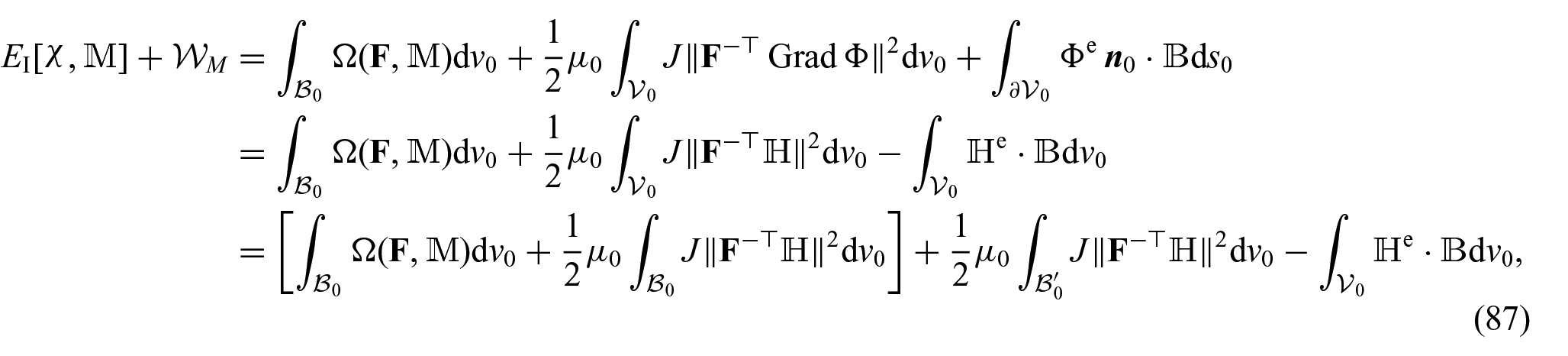
6.2. Potential energy functionals based on $\mathbb{M},\overline{\mathbb{M}}$ and $\mathbb{K}$

Following the arguments in Section 4, we assumed that

$$\mathcal{V}={\mathcal{V}}_0={\mathbb{R}}^3,$$

(98)

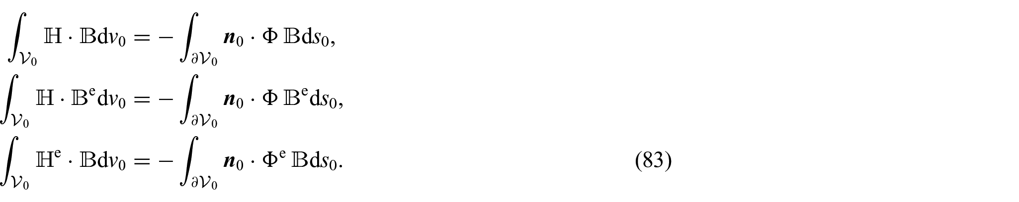
for the formulation presented in Section 3. This needed some changes in equation (18). Clearly, the only term that needs to be rewritten is the last term in equation (18). Using the nature of a magnetic field in vacuum we have, by equation (83),

$${\int }_{\partial {\mathcal{V}}_0}{\varphi }^{\mathrm{e}}{\mathit{n}}_0·\mathbb{B}\mathrm{d}{s}_0=-{\int }_{{\mathcal{V}}_0}{\mathbb{H}}^{\mathrm{e}}·\mathbb{B}\mathrm{d}{v}_0.$$

Hence, based on equations (18) and (41), we get

$$\begin{array}{c}{E}_{\mathrm{I}}-E_{\mathrm{II}}=E_{\mathrm{I}}[\chi ,\mathbb{M}]-E_{\mathrm{II}}[\chi ,\overline{\mathbb{M}}]\hfill \\ ={\int }_{{\mathcal{B}}_0}[\mathrm{\Omega }(\mathbf{F},\mathbb{M})-{\rho }_0\hat{\mathrm{\Omega }}(\mathbf{F},\overline{\mathbb{M}})+{\rho }_{0}J{\mathbb{h}}^{\mathrm{e}}(\chi (\mathit{X}))·{\mathbf{F}}^{-\mathrm{T}}\overline{\mathbb{M}}]\mathrm{d}{v}_0+\frac{{\mu }_0}{2}{\int }_{{\mathcal{V}}_0}J{\mathbf{C}}^{-1}\mathbb{H}·\mathbb{H}\mathrm{d}{v}_0-{\int }_{{\mathcal{V}}_0}{\mathbb{H}}^{\mathrm{e}}·\mathbb{B}\mathrm{d}{v}_0\hfill \\ -\frac{1}{2}{\mu }_0{\int }_{{\mathcal{B}}_0}J{\mathbf{C}}^{-1}{\mathbb{H}}^{\mathrm{s}}·{\mathbb{H}}^{\mathrm{s}}\mathrm{d}{v}_0-\frac{1}{2}{\mu }_0{\int }_{\mathcal{B}{\prime }_0}J{\mathbf{C}}^{-1}{\mathbb{H}}^{\mathrm{s}}·{\mathbb{H}}^{\mathrm{s}}\mathrm{d}{v}_0.\hfill \end{array}$$

(99)

The first term in the second line can be rewritten in view of equation (16) as

$$\frac{{\mu }_0}{2}{\int }_{{\mathcal{V}}_0}J{\mathbf{C}}^{-1}\mathbb{H}·\mathbb{H}\mathrm{d}{v}_0=\frac{{\mu }_0}{2}{\int }_{{\mathcal{V}}_0}J{\mathbf{C}}^{-1}[{\mathbb{H}}^{\mathrm{e}}·{\mathbb{H}}^{\mathrm{e}}+2{\mathbb{H}}^{\mathrm{e}}·{\mathbb{H}}^{\mathrm{s}}+{\mathbb{H}}^{\mathrm{s}}·{\mathbb{H}}^{\mathrm{s}}]\mathrm{d}{v}_0.$$

(100)

On substituting this back into equation (99), we get

$$\begin{array}{c}{E}_{\mathrm{I}}-E_{\mathrm{II}}={\int }_{{\mathcal{B}}_0}[\mathrm{\Omega }(\mathbf{F},\mathbb{M})-{\rho }_0\hat{\mathrm{\Omega }}(\mathbf{F},\overline{\mathbb{M}})+{\rho }_{0}J{\mathbb{h}}^{\mathrm{e}}(\chi (\mathit{X}))·{\mathbf{F}}^{-\mathrm{T}}\overline{\mathbb{M}}]\mathrm{d}{v}_0+{\mu }_0{\int }_{{\mathcal{V}}_0}J{\mathbf{C}}^{-1}{\mathbb{H}}^{\mathrm{e}}·{\mathbb{H}}^{\mathrm{s}}\mathrm{d}{v}_0\hfill \\ +\frac{{\mu }_0}{2}{\int }_{{\mathcal{V}}_0}J{\mathbf{C}}^{-1}{\mathbb{H}}^{\mathrm{e}}·{\mathbb{H}}^{\mathrm{e}}\mathrm{d}{v}_0-{\int }_{{\mathcal{V}}_0}{\mathbb{H}}^{\mathrm{e}}·{\mathbb{B}}^{\mathrm{s}}\mathrm{d}{v}_0-{\mu }_0{\int }_{{\mathcal{V}}_0}J{\mathbf{C}}^{-1}{\mathbb{H}}^{\mathrm{e}}·{\mathbb{H}}^{\mathrm{e}}\mathrm{d}{v}_0\hfill \end{array}$$

(101)

$$\begin{array}{c}={\int }_{{\mathcal{B}}_0}[\mathrm{\Omega }(\mathbf{F},\mathbb{M})-{\rho }_0\hat{\mathrm{\Omega }}(\mathbf{F},\overline{\mathbb{M}})+{\rho }_{0}J{\mathbb{h}}^{\mathrm{e}}(\chi (\mathit{X}))·{\mathbf{F}}^{-\mathrm{T}}\overline{\mathbb{M}}]\mathrm{d}{v}_0-{\int }_{{\mathcal{B}}_0}J{\mathbf{C}}^{-1}{\mathbb{H}}^{\mathrm{e}}·\mathbb{M}\mathrm{d}{v}_0\hfill \\ -\frac{{\mu }_0}{2}{\int }_{{\mathcal{V}}_0}J{\mathbf{C}}^{-1}{\mathbb{H}}^{\mathrm{e}}·{\mathbb{H}}^{\mathrm{e}}\mathrm{d}{v}_0.\hfill \end{array}$$

(102)

Since $\mathbb{M}={\rho }_0\overline{\mathbb{M}}$ and ${\mathbb{H}}^{\mathrm{e}}={\mathbf{F}}^{\mathrm{T}}{\mathbb{h}}^{\mathrm{e}}$ , this can be rewritten as

$$E_{\mathrm{I}}-E_{\mathrm{II}}={\int }_{{\mathcal{B}}_0}[\mathrm{\Omega }(\mathbf{F},\mathbb{M})-{\rho }_0\hat{\mathrm{\Omega }}(\mathbf{F},\overline{\mathbb{M}})]\mathrm{d}{v}_0-\frac{{\mu }_0}{2}{\int }_{{\mathcal{V}}_0}J{\mathbf{C}}^{-1}{\mathbb{H}}^{\mathrm{e}}·{\mathbb{H}}^{\mathrm{e}}\mathrm{d}{v}_0.$$

(103)

Thus, the two potential energies differ not only by the definition of the respective stored energy density functions but also by an extra term; the latter term, clearly, is a constant term, though it could be infinite for ${\mathbb{H}}^{\mathrm{e}}\ne 0$ while the former can be made zero by naturally identifying the stored energy density functions.

From equations (41) and (70) (using equation (69)), we get

$$E_{\mathrm{II}}[\chi ,\overline{\mathbb{M}}]-E_{\mathrm{III}}[\chi ,\mathbb{K}]={\int }_{{\mathcal{B}}_0}{\rho }_0[\hat{\mathrm{\Omega }}(\mathbf{F},\overline{\mathbb{M}})-\tilde{\mathrm{\Omega }}(\mathbf{F},\mathbb{K})]\mathrm{d}{v}_0.$$

(104)

These two potential energies differ only by the definition of the respective stored energy density functions, which can be naturally identified to achieve an equivalence.

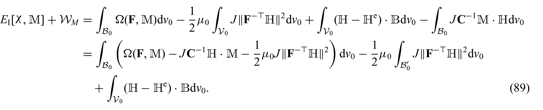
6.3. Comparison with the expressions provided by [13] using a modified potential energy functional

Since ${\mathbb{h}}^{\mathrm{e}}$ is the gradient of a potential, and in view of equation (15), by a direct calculation, we have ${\int }_{{\mathbb{R}}^3}{\mathbb{h}}^{\mathrm{e}}·{\mathbb{b}}^{\mathrm{s}}\mathrm{d}v=0$ , as a result of which we get

$${\int }_{{\mathcal{B}}_0}{\rho }_0{\mathbb{h}}^{\mathrm{e}}·\mathbb{K}\mathrm{d}{v}_0={\int }_{\mathcal{B}}{\mathbb{h}}^{\mathrm{e}}·\mathrm{md}v={\int }_{{\mathbb{R}}^3}{\mathbb{h}}^{\mathrm{e}}·({\mathbb{b}}^{\mathrm{s}}-{\mu }_0{\mathbb{h}}^{\mathrm{s}})\mathrm{d}v=-{\mu }_0{\int }_{{\mathbb{R}}^3}{\mathbb{h}}^{\mathrm{e}}·{\mathbb{h}}^{\mathrm{s}}\mathrm{d}v.$$

(105)

Note that ${\mu }_0{\int }_{{\mathbb{R}}^3}{\mathbb{h}}^{\mathrm{e}}·{\mathbb{h}}^{\mathrm{s}}\mathrm{d}v$ is nonzero; indeed, with ${\mathbb{h}}^{\mathrm{s}}=-\mathrm{grad}{\varphi }^{\mathrm{s}}$ , ${\mu }_0{\mathbb{h}}^{\mathrm{e}}={\mathbb{b}}^{\mathrm{e}}$ and $B_r\subset {\mathbb{R}}^3$ as a ball of radius $r$ , we find it to be equal to

$$-{\int }_{{\mathbb{R}}^3}{\mathbb{b}}^{\mathrm{e}}·\mathrm{grad}{\varphi }^{\mathrm{s}}\mathrm{d}v=\underset{r\to \infty }{lim}[{\int }_{B_r}\mathrm{div}{\mathbb{b}}^{\mathrm{e}}{\varphi }^{\mathrm{s}}\mathrm{d}v-{\int }_{\partial B_r}{\varphi }^{\mathrm{s}}{\mathbb{b}}^{\mathrm{e}}·{\mathit{n}}_0\mathrm{d}s],$$

where $\mathrm{div}{\mathbb{b}}^{\mathrm{e}}=0$ in the first term but ${\varphi }^{\mathrm{s}}$ may not necessarily go to zero in the second term as $r=\parallel \mathit{x}\parallel \to \infty$ . Thus, an equivalent potential energy functional is

$$E_{\mathrm{III}}(\chi ,\mathbb{K})+{\int }_{{\mathcal{B}}_0}{\rho }_0{\mathbb{h}}^{\mathrm{e}}·\mathbb{K}\mathrm{d}{v}_0+{\mu }_0{\int }_{{\mathbb{R}}^3}{\mathbb{h}}^{\mathrm{e}}·{\mathbb{h}}^{\mathrm{s}}\mathrm{d}v,$$

in addition to which by including the constant term $\frac{1}{2}{\mu }_0{\int }_{{\mathbb{R}}^3}{\mathbb{h}}^{\mathrm{e}}·{\mathbb{h}}^{\mathrm{e}}\mathrm{d}v$ too, we get (recall equation (36))

$$\overline{E_{\mathrm{III}}}(\chi ,\overline{\mathbb{m}})={\int }_{\mathcal{B}}\rho \hat{\mathrm{\Omega }}(\mathbf{F},\overline{\mathbb{m}})\mathrm{d}v+{\mathcal{W}}_M+\frac{1}{2}{\mu }_0{\int }_{\mathcal{B}}\mathbb{h}·\mathrm{hd}v+\frac{1}{2}{\mu }_0{\int }_{\mathcal{B}\prime }\mathbb{h}·\mathrm{hd}v,$$

(106)

with its referential form (to be compared with equation (70)) as

$$\widehat{E_{\mathrm{III}}}(\chi ,\mathbb{K})={\int }_{{\mathcal{B}}_0}{\rho }_0\tilde{\mathrm{\Omega }}(\mathbf{F},\mathbb{K})\mathrm{d}{v}_0+{\mathcal{W}}_M+\frac{1}{2}{\mu }_0{\int }_{{\mathcal{B}}_0}J{\mathbf{C}}^{-1}\mathbb{H}·\mathbb{H}\mathrm{d}{v}_0+\frac{1}{2}{\mu }_0{\int }_{\mathcal{B}{\prime }_0}J{\mathbf{C}}^{-1}\mathbb{H}·\mathbb{H}\mathrm{d}{v}_0.$$

(107)

This expression coincides with the potential energy functional of equation (18) except for the last term (which is absent in the present scenario as $\mathcal{V}={\mathbb{R}}^3$ ) and, more importantly, a different measure of magnetisation; note that

$$\mathbb{K}(\mathit{X})=\overline{\mathbb{m}}(\mathit{x})={\rho }^{-1}(\mathit{x}){\mathbf{F}}^{-\mathrm{T}}(\mathit{X})\mathbb{M}(\mathit{X})$$

by equations (12) and (13). Like equation (71), we have

$$\delta \mathbb{B}=[[{\mathbf{F}}^{-\mathrm{T}}·\delta \mathbf{F}]\mathbf{I}-{\mathbf{C}}^{-1}\delta {\mathbf{F}}^{\mathrm{T}}\mathbf{F}]{\mu }_{0}J{\mathbf{C}}^{-1}\mathbb{H}-{\mathbf{F}}^{-1}\delta \mathbf{F}\mathbb{B}-{\mu }_{0}J{\mathbf{C}}^{-1}\mathrm{Grad}\delta \mathrm{\Phi }+{\rho }_0{\mathbf{F}}^{-1}\delta \mathbb{K},$$

(108)

and like equation (48) we have (with $B_R\subset {\mathbb{R}}^3$ as a ball of radius $R$ )

$$\begin{array}{c}-{\int }_{{\mathcal{B}\prime }_0}\mathbb{H}·\delta \mathbb{B}\mathrm{d}{v}_0={\int }_{{\mathcal{B}\prime }_0}\mathrm{Grad}\mathrm{\Phi }·\delta \mathbb{B}\mathrm{d}{v}_0\hfill \\ =\underset{R\to \infty }{lim}({\int }_{\partial B_R}\mathrm{\Phi }{\mathit{n}}_0·\delta \mathbb{B}\mathrm{d}{s}_0-{\int }_{B_R}\mathrm{\Phi }\mathrm{div}\delta \mathbb{B}\mathrm{d}{v}_0)-{\int }_{\partial {\mathcal{B}}_0}{\mathit{n}}_0·\mathrm{\Phi }\delta \mathbb{B}\mathrm{d}{s}_0\hfill \\ =-{\int }_{\partial {\mathcal{B}}_0}{\mathit{n}}_0·\mathrm{\Phi }\delta \mathbb{B}\mathrm{d}{s}_0,\hfill \end{array}$$

(109)

assuming that $\delta \mathbb{B}·{\mathit{n}}_0$ vanishes as $R=\parallel \mathit{X}\parallel \to \infty$ in a suitable manner. By carrying out the first variation analysis, similar to that presented earlier in this section, we get

$$\begin{array}{c}\delta \widehat{E_{\mathrm{III}}}(\chi ,\mathbb{K})={\int }_{{\mathcal{B}}_0}{\rho }_0[{\tilde{\mathrm{\Omega }}}_{,\mathbf{F}}·\delta \mathbf{F}+{\tilde{\mathrm{\Omega }}}_{,\mathbb{K}}·\delta \mathbb{K}]\mathrm{d}{v}_0-{\int }_{{\mathcal{B}}_0}{\tilde{\mathit{f}}}^{\mathrm{e}}·\delta \chi \mathrm{d}{v}_0-{\int }_{\partial {\mathcal{B}}_0}{\tilde{\mathit{t}}}^{\mathrm{e}}·\delta \chi \mathrm{d}{s}_0+{\int }_{{\mathcal{B}}_0}(-{\hat{\mathbf{P}}}_m·\delta \mathbf{F})\mathrm{d}{v}_0\hfill \\ +{\int }_{\mathcal{B}{\prime }_0}(-{\hat{\mathbf{P}}}_m·\delta \mathbf{F})\mathrm{d}{v}_0+{\int }_{{\mathcal{B}}_0}{\stackrel{°}{\mathbf{P}}}_m·\delta \mathbf{F}\mathrm{d}{v}_0-{\int }_{{\mathcal{B}}_0}{\mathbb{H}}^{\mathrm{s}}·({\rho }_0{\mathbf{F}}^{-1}\delta \mathbb{K})\mathrm{d}{v}_0-{\int }_{\partial {\mathcal{B}}_0}{\mathit{n}}_0·{\mathrm{\Phi }}^{\mathrm{s}}\delta {\mathbb{B}}^{\mathrm{s}}\mathrm{d}{s}_0\hfill \\ +{\int }_{{\mathcal{B}\prime }_0}{\stackrel{°}{\mathbf{P}}}_m·\delta \mathbf{F}\mathrm{d}{v}_0+{\int }_{\partial {\mathcal{B}}_0}{\mathit{n}}_0·{\mathrm{\Phi }}^{\mathrm{s}}\delta {\mathbb{B}}^{\mathrm{s}}\mathrm{d}{s}_0,\hfill \end{array}$$

(110)

where ${\hat{\mathbf{P}}}_m$ is defined by equation (21) and ${\stackrel{°}{\mathbf{P}}}_m$ is defined by equation (26). The Euler–Lagrange equations by setting $\delta \widehat{E_{\mathrm{III}}}=0$ are derived as

$$\mathrm{Div}\left(\mathbf{P}\right)+{\tilde{\mathit{f}}}^{\mathrm{e}}=0\mathrm{in}{\mathcal{B}}_0,$$

(111a)

$$\left[\left[\mathbf{P}\right]\right]{\mathit{n}}_0+{\tilde{\mathit{t}}}^{\mathrm{e}}=0\mathrm{on}\partial {\mathcal{B}}_0,$$

(111b)

$$\mathrm{Div}\left(\mathbf{P}\right)=0\mathrm{in}\mathcal{B}{\prime }_0,$$

(111c)

$$\mathbf{F}{\mathbb{H}}^{\mathrm{s}}={\tilde{\mathrm{\Omega }}}_{,\mathbb{K}}\mathrm{in}{\mathcal{B}}_0,$$

(111d)

by recognising that, for this potential energy functional, the first Piola–Kirchhoff stress is given by

$$\mathbf{P}={\rho }_0{\tilde{\mathrm{\Omega }}}_{,\mathbf{F}}+{\stackrel{°}{\mathbf{P}}}_m-{\hat{\mathbf{P}}}_m\mathrm{in}{\mathcal{B}}_0,$$

(112a)

$$\mathbf{P}={\stackrel{°}{\mathbf{P}}}_m-{\hat{\mathbf{P}}}_m\mathrm{in}\mathcal{B}{\prime }_0.$$

(112b)

On a direct comparison of these equations with equations (77) and (78), we note that, owing to the inclusion of extra terms with ${\mathbb{h}}^{\mathrm{e}}$ , the expressions for first Piola–Kirchhoff stress and the Maxwell stress in vacuum are different. This leads to the vanishing of the equivalent of electromagnetic body force term in equation (111a) and a modified constitutive equation (equation (111d)).

7. Concluding remarks

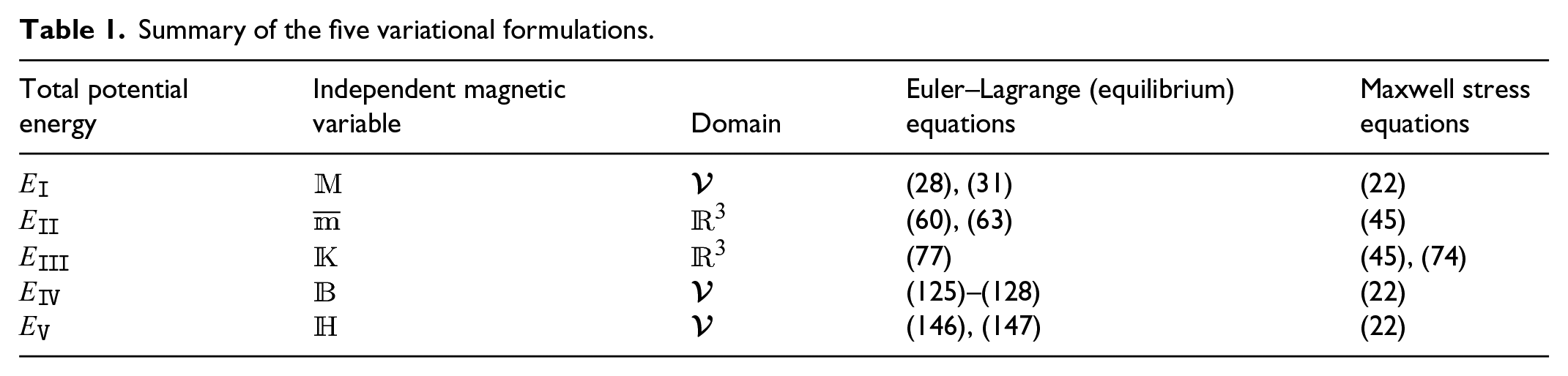
In this paper, we present five variational formulations of nonlinear magnetoelastostatics that differ from each other with respect to the independent field variable for the magnetic effect. The formulations based on the magnetic field $\mathbb{H}$ , the magnetic induction $\mathbb{B}$ and the referential magnetisation vector per unit volume $\mathbb{M}$ are analogous to the variational formulations of electroelastostatics presented by Saxena and Sharma [33]. Variational formulation based on referential magnetisation per unit mass $\overline{\mathbb{M}}$ was originally postulated by Brown [32] and that based on a pull-back of the magnetisation per unit mass to reference configuration $\mathbb{K}$ was given by Kankanala and Triantafyllidis [13]. A direct equivalence between all five principles by means of the Legendre transform and the properties of Maxwell equations is the highlight of Section 6 of this paper.

The principles can broadly be divided into two categories. For the first kind, based on $\mathbb{H},\mathbb{B}$ and $\mathbb{M}$ , the total energy is defined over a bounded domain $\mathcal{V}$ , with the external magnetic loading being specified by means of the potential on the boundary $\partial \mathcal{V}$ . For the second kind, based on $\overline{\mathbb{M}}$ and $\mathbb{K}$ , the integral is defined over an infinite space and the notion of an external field becomes necessary to supply external loading. The choice to include this (constant) external field in the total energy can lead to a different definition of the Maxwell stress, and result in changes in the body force and traction terms. A summary of these principles is presented in Table 1 for easy reference. Our analysis suggests caution with the choice of variational principle appropriate to the physical problem and control variables.

Table 1.

Summary of the five variational formulations.

Total potential energy	Independent magnetic variable	Domain	Euler–Lagrange (equilibrium) equations	Maxwell stress equations
$E_{\mathrm{I}}$	$\mathbb{M}$	$\mathcal{V}$	(28), (31)	(22)
$E_{\mathrm{II}}$	$\overline{\mathbb{m}}$	${\mathbb{R}}^3$	(60), (63)	(45)
$E_{\mathrm{III}}$	$\mathbb{K}$	${\mathbb{R}}^3$	(77)	(45), (74)
$E_{\mathrm{IV}}$	$\mathbb{B}$	$\mathcal{V}$	(125)–(128)	(22)
$E_{\mathrm{V}}$	$\mathbb{H}$	$\mathcal{V}$	(146), (147)	(22)

The analysis presented in this paper can be easily extended to the special case of incompressibility. For this purpose, see Remark 4 in the recent exposition and formulation for the electroelastic counterpart [33]. Further extension of the present analysis to include mixed boundary conditions and discontinuities in the magnetoelastic body or free space can shed further light on the issues around correspondences between the five principles. Inclusion of kinetic energy and the effect of time-dependent boundaries is another possible interesting area for extension of the analysis presented here. We have restricted our analysis to nonlinear deformation and coupling. A linearised analysis to study deformation close to the reference configuration may lead to simplifications and influence the equivalence analysis presented in Section 6. These avenues are currently under investigation and shall appear in suitable form elsewhere.