
Abstract
Input–output partial feedback linearisation is experimentally implemented on a non-smooth nonlinear system without the necessity of a conventional system matrix model for the first time. The experimental rig consists of three lumped masses connected and supported by springs with low damping. The input and output are at the first degree of freedom with a non-smooth clearance-type nonlinearity at the third degree of freedom. Feedback linearisation has the effect of separating the system into two parts: one linear and controllable and the other nonlinear and uncontrollable. When control is applied to the former, the latter must be shown to be stable if the complete system is to be stable with the desired dynamic behaviour.
1. Introduction
The classical feedback linearisation method, well-known through text books such as [1–3], requires the use of a numerical model of the system. It is generally applicable to under-actuated systems and, by an application of a linear transformation, the system is separated into two parts. An artificial input is applied to the first part that renders it linear and enables classical linear control methods, such as pole placement, to be applied. The second part generally remains nonlinear and is rendered uncontrollable by the transformation. The stability of the second part is guaranteed when the zero dynamics (i.e. the second part with the controlled coordinates set to zero and subject to arbitrary disturbance) are stable. The method of receptances is an active control method that makes use of measurements acquired directly from the test structure and therefore eliminates the necessity of evaluating the system mass, damping and stiffness matrices
Classical feedback linearisation has found application in several areas. In the field of aeroelasticity, a series of papers [6–11] demonstrated theoretical and experimental application of the method to successfully control a pitch-plunge aeroelastic system. A recent publication by Jiffri et al. [12] followed a similar control approach, but with the inclusion of a real-time embedded tuned numerical model of the aeroelastic system in the control scheme. More recently, Castillo-Berrio and Feliu-Batlle [13] applied feedback linearisation experimentally to achieve precise beam-tip position control in a nonlinear two degrees of freedom flexible-beam sensor. A similar position control application was presented in [14], where Nanos and Papadopoulos applied feedback linearisation to ensure accurate path following of a space manipulator in the presence of joint flexibilities, which also had the effect of mitigating vibrations transmitted to the spacecraft supporting the manipulator. Choi and Ahn [15] experimentally implemented a feedback linearisation based controller for successful position and attitude control of a quadcopter. Alonge et al. [16] presented the theoretical development of a feedback linearisation based controller for the control of linear induction motor (LIM) drives with dynamic end effects which give rise to significant nonlinear behaviour. These results were later validated through experimental tests [17], which showed significant improvements when feedback linearisation was applied adaptively.
The application of classical input-output partial feedback linearisation was extended to systems with non-smooth nonlinearities by Jiffri et al. [18]. Experimental application of the method to the three degrees of freedom system discussed in this paper was successfully achieved by the present authors [19, 20], but significant effort was required to tune the numerical model to an adequate level of accuracy, in both the linear and nonlinear parameters, to successfully achieve the desired closed-loop dynamics. A special case was considered by Lisitano et al. [19] whereby control was applied to the same degree of freedom as the nonlinearity. In such a case, the system is linearised completely and the problem of determining the zero dynamics is trivialised to a check that the system is minimum phase. Lisitano et al. [20] considered the case when the nonlinearity was located at a different position, requiring a detailed and complex analysis to be carried out to establish the zero dynamics. The stability of the zero dynamics can alternatively be verified using the receptance method with a describing function (DF) approach [21], either using an analytical DF (as in the present case) or by carrying out a series of slow-sweep amplitude-controlled sine-excitation tests. An exposition of the theory of feedback linearisation by the receptance method was recently presented by Zhen et al. [22], and the purpose of the present paper is to demonstrate experimentally their findings, using the approach presented in that paper to replicate the closed-loop results already obtained for the three degrees of freedom test-rig with classical feedback linearisation by Lisitano et al. [20].
The subject of friction and impact in non-smooth nonlinear mechanical systems has long been studied by engineering scientists. For example, in 1995 Canudas de Wit et al. [23] combined the Dahl and Stribeck effects in a single model to represent both the effects of ‘stiction’ and decreasing friction with increasing velocity. They used the model to construct a friction observer and to carry out friction compensation in a tracking controller. More recently Giorgio and Scerrato [24] developed a multi-scale model, consisting of macro-, meso- and micro-scales, to represent rate-dependent internal friction in concrete. At the micro-scale, the model was of the Lu-Gre type that accounts for Coulomb friction and includes the Stribeck effect. Andreaus et al. [25] considered the dynamics of a cantilever beam that made contact with an obstacle in the form of a spring and viscous damper. Rather than an instantaneous impact, their model allowed for contact forces of finite duration governed by Heaviside functions, a single Heaviside function for the contact stiffness and double Heaviside functions for the contact damping. The resulting nonlinear differential equations were integrated numerically and validated by experiments. The same authors considered the microcantilever dynamics in tapping mode atomic force microscopy [26] including the van-der-Waals and Derjaguin–Muller–Toporov (DMT) contact forces.
In the present work, the form of the non-smooth nonlinearity is a piecewise stiffness (and damping) nonlinearity formed by the closure and opening of two gaps on either side of a linear spring. The stiffness is increased when the gap closes on one side and between the gaps the stiffness is linear. Friction is present during the periods that either gap is closed; its effect is represented by a Coulomb-type damping force proportional to the absolute stiffness force and directed in opposition to velocity. The effects of an instantaneous impact are neglected.
This paper is organised as follows. The experimental arrangement of the three degrees of freedom non-smooth nonlinear system is described in section 2 together with its actuation and sensors. In section 3, the system model, based on measured receptance data, and the complex DF with stiffness and damping terms is presented. Feedback linearisation theory is briefly described in section 4. In section 5 the results of preliminary tests are presented, showing inverse receptance terms, required by the theory, and the eigenvalues of the zero dynamics for different amplitudes of sinusoidal displacement. Finally, in section 6, the results of experimental implementation of the receptance-based feedback linearisation method are presented, both in the frequency and time domains.
2. Experimental arrangement
The experimental system shown in Figure 1 consists of three masses, degrees of freedom 1, 2 and 3 from left to right, supported and connected by thin plate-like springs. The system includes a non-smooth structural nonlinearity in the form of a piecewise-linear spring arrangement located at the third degree of freedom. This is achieved by adding two springs, known as setting springs, mounted on either side of the third mass with continuously adjustable separation (gaps
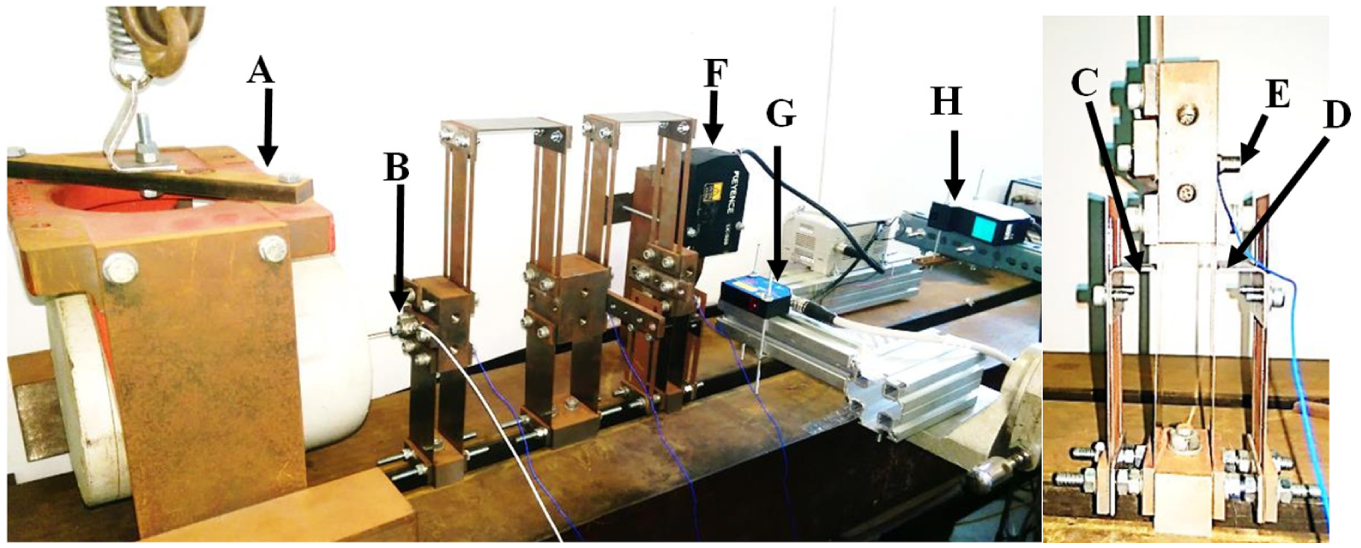
Non-smooth nonlinear system experimental setup. A: Suspended Shaker. B: Load cell. C: Left gap g1. D: Right gap g2. E:Accelerometers. F: Laser q1. G: Laser q2. H: Laser q3.
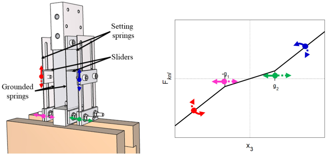
Nonlinear spring model (left), nonlinear spring characteristic (right).
Excitation could be applied either by an instrumented hammer (PCB 086C03) or the suspended shaker (LDS V406) with the LDS PA100 amplifier. Load cell PCB 208C02 was used to measure the force applied by the shaker with PCB 442C04 ICP signal conditioner. Laser displacement measurements (Keyence LK-500 and LK-G402, and microepsilon OptoNCDT 1402-100) were available and acceleration sensors (K-Shear 8728A500) were mounted on each of the three masses with PCB 442C04 ICP signal conditioners. Displacements and velocities were used in control experiments with velocities determined by numerical differentiation of laser displacement measurements.
Hammer excitation and accelerometers were used with a Siemens LMS Test.Lab system for the determination of receptances for the underlying linear system (i.e. with the setting springs removed) and for the partially linearised closed-loop system. The closed-loop control force was applied using the shaker, and implemented using dSPACE (10 kHz sampling speed) within a nested controller, as shown in Figure 3. The inner PD loop is present to ensure that the desired control force has indeed been applied, this being necessary because the shaker is current controlled and therefore its force is not proportional to the dSPACE command voltage. A Butterworth filter with a cut-off frequency of 21 Hz was used to remove high frequency noise and the saturator shown in the figure was present to prevent damage that might otherwise be caused to the shaker should the armature hit the end stops.
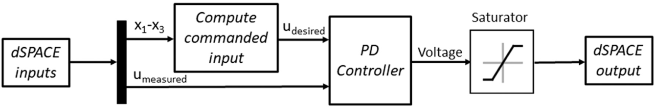
Nested controller.
3. Receptance-based model
The system may be represented as shown in Figure 4, as a three degrees of freedom arrangement of lumped masses connected by springs and light dampers. It is seen that one of the two springs labelled
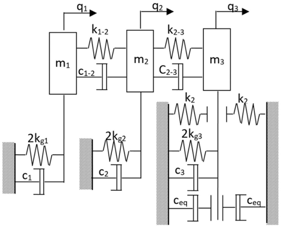
Schematic of the three degrees of freedom non-smooth nonlinear system.
One advantage of the receptance method is that a mathematical model of the usual

and, in the Laplace ‘s’ domain by modal synthesis
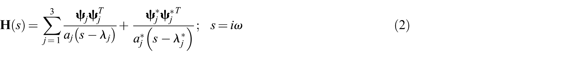
where
If the displacement of

where

and the sweep rate, Ω, is very low in comparison to the natural frequencies of the system.
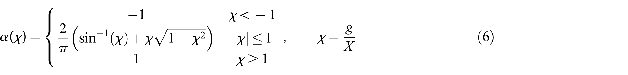
Equations (3) and (4) are the equivalent of the DF representation of stiffness

where
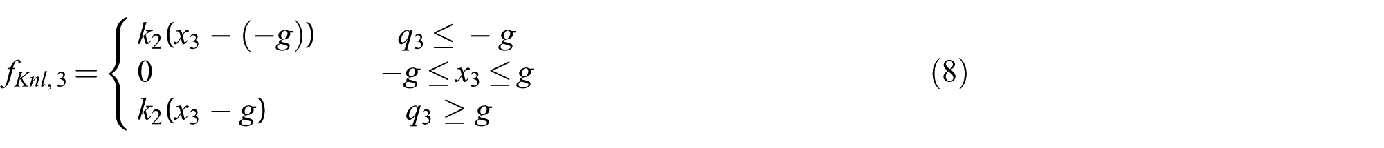
The nonlinear damper force was represented using a Coulomb model by the present authors as

where
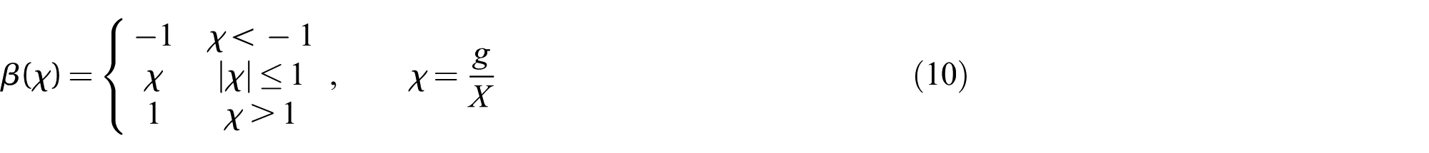
The DF for the nonlinear damper is developed in the Appendix and given here as

where
Thus. the total DF, including stiffness and damping is

or, when written in the Laplace ‘s’ domain,

If the linear receptance matrix, equation (1) is available and the DF known, then the amplitude-dependent receptance, equation (3), may be computed by using the Sherman–Morrison formula [27, 28]

where
4. Feedback linearisation by the method of receptances
The theory of feedback linearisation by the receptance method is given in detail by Zhen et al. [22]. A summary is provided here for purposes of completeness. To begin, equation (1) may be re-written in the form

where

and the output is given by

A coordinate transformation is then defined with the purpose of separating the system into two parts, controllable and uncontrollable, known as the normal form. Thus

where

In the case of the three degrees of freedom system shown in Figure 4, the terms in equations (17) and (18) are given by,
Then, in transformed coordinates and using partitioning consistent with that in equations (15) and (17),

where

Inverting equation (19) leads to
and, if the control input is chosen, as

then the first row of equation (21) is linearised and may be written as

where
A pole

and control gains

For the system to be stable, not only must the poles of the controllable part be stable, but also the so-called zero dynamics must be stable. The zero dynamics are those of the uncontrollable system (known as the internal dynamics) when the controlled degrees of freedom are set to zero. Zhen et al. [22] showed that the zero dynamics were stable if, and only if, the poles of the transfer function

are stable for the range of all amplitudes
5. Preliminary tests
Experimental and synthesised frequency response functions (using equation (2)) of the underlying linear system are presented in Figure 5, where very close agreement can be observed.
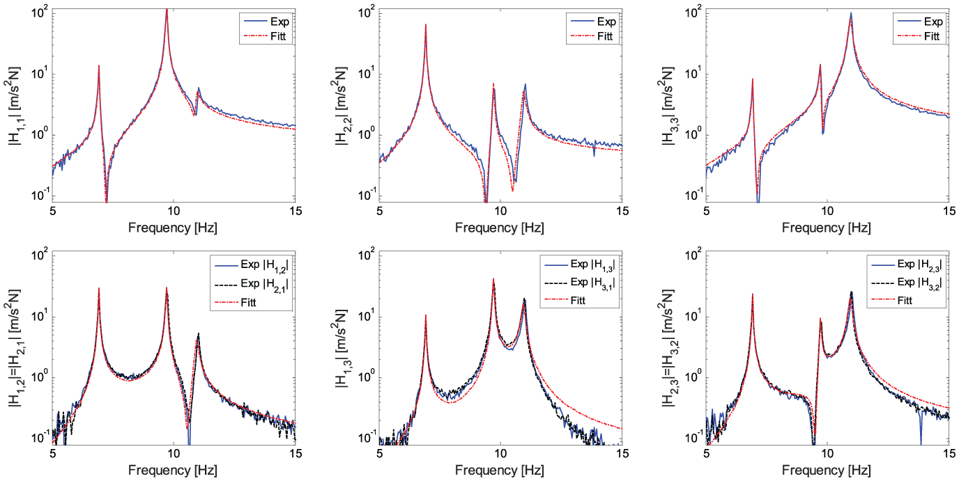
Experimental and synthesised FRFs.
Elements of the inverse receptance matrix (i.e. the experimental dynamic stiffness matrix) are required in equations (22) and (26) and shown in Figure 6, where inversion of both the measured and synthesised FRFs are shown to be in almost perfect agreement.
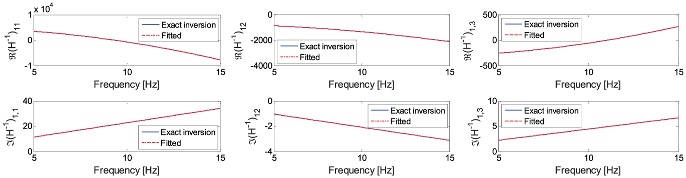
Inverse receptance terms (dynamic stiffness).
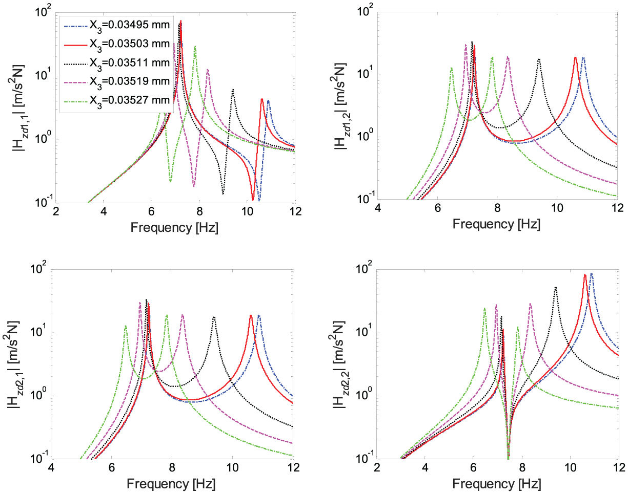
The nonlinear receptances obtained from equation (13) for different values of
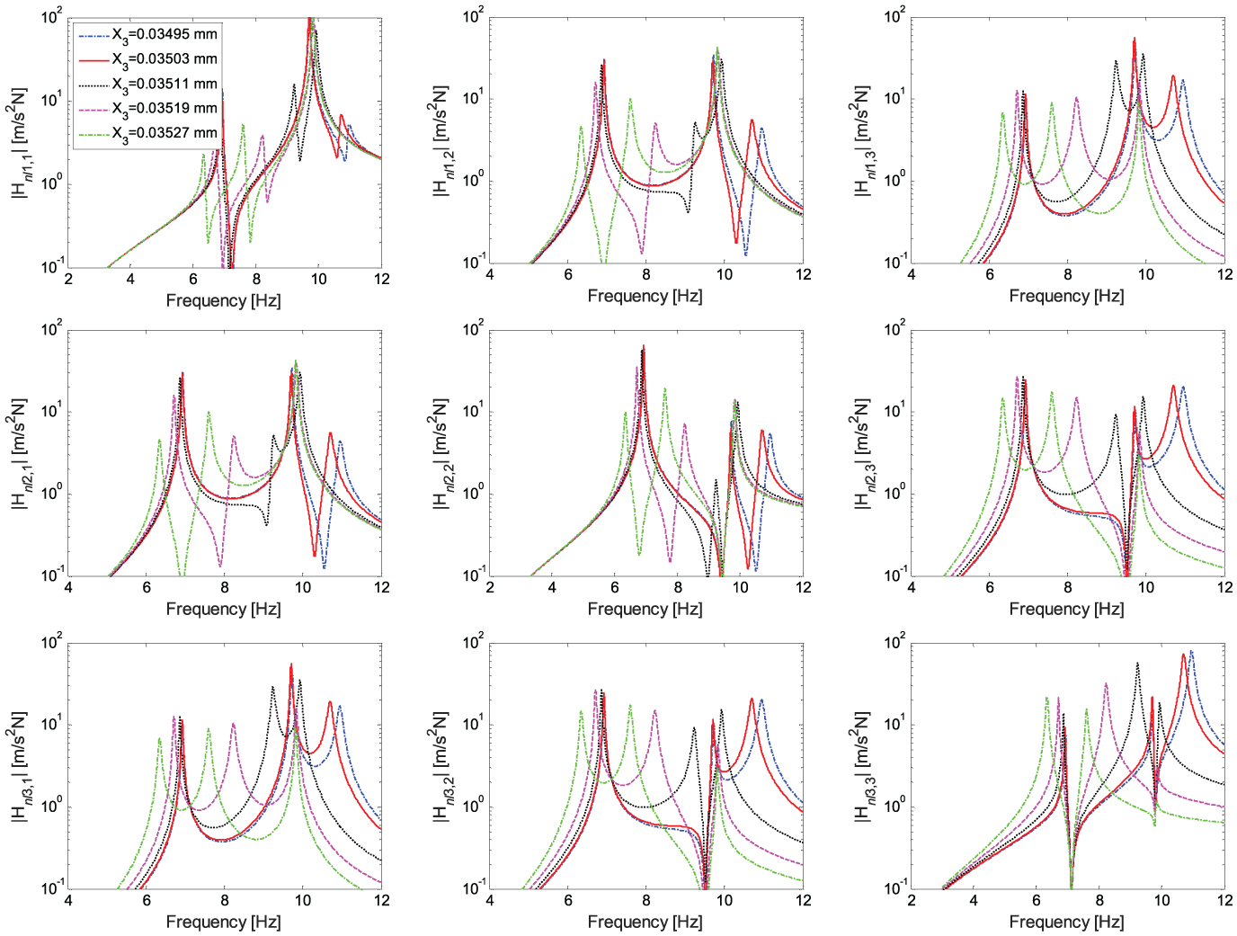
FRF matrix of the nonlinear system, changing amplitude.
The transfer function matrix of the zero dynamics determined by using the amplitude-dependent receptances in equation (26) are shown in Figure 8. The loci of the zero dynamics poles, extracted by using rational fractional polynomials, are shown in Figure 9, and Figure 10 shows an enlarged view close to the gap at X=0.035 mm.
Zero dynamics FRF changing
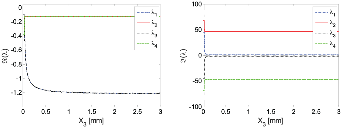
Poles of the zero dynamics: real part (left), imaginary part (right).
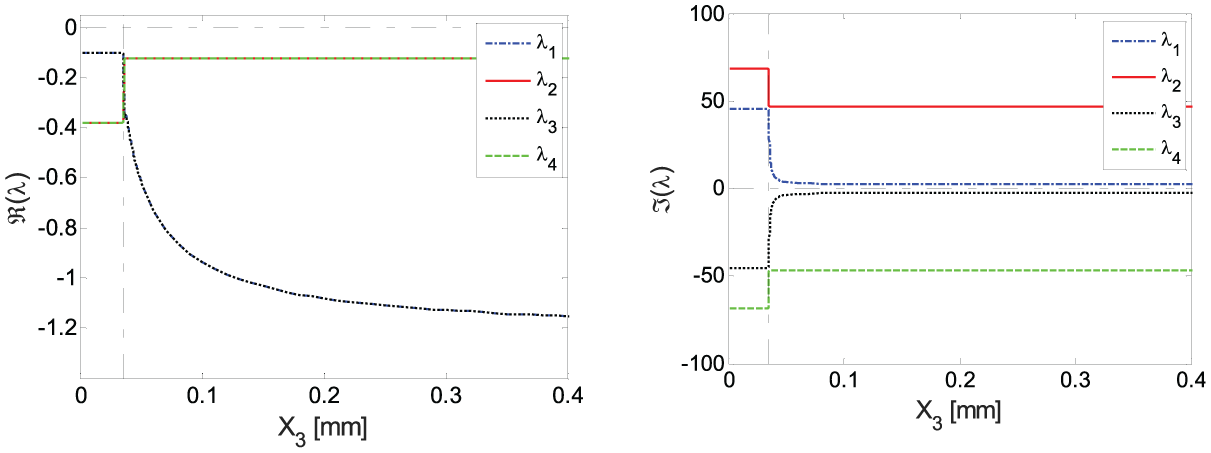
Zoomed view of poles: real part (left), imaginary part (right).
Having established that the zero dynamics are stable, pole placement may be carried out as described in the following section.
6. Results from the closed-loop system
In this section, experimental results produced by the receptance-based partial feedback linearisation approach described in section 4 are presented and compared to numerically-produced results from a
Experiments and numerical simulations were repeated for three different values of assigned natural frequencies,
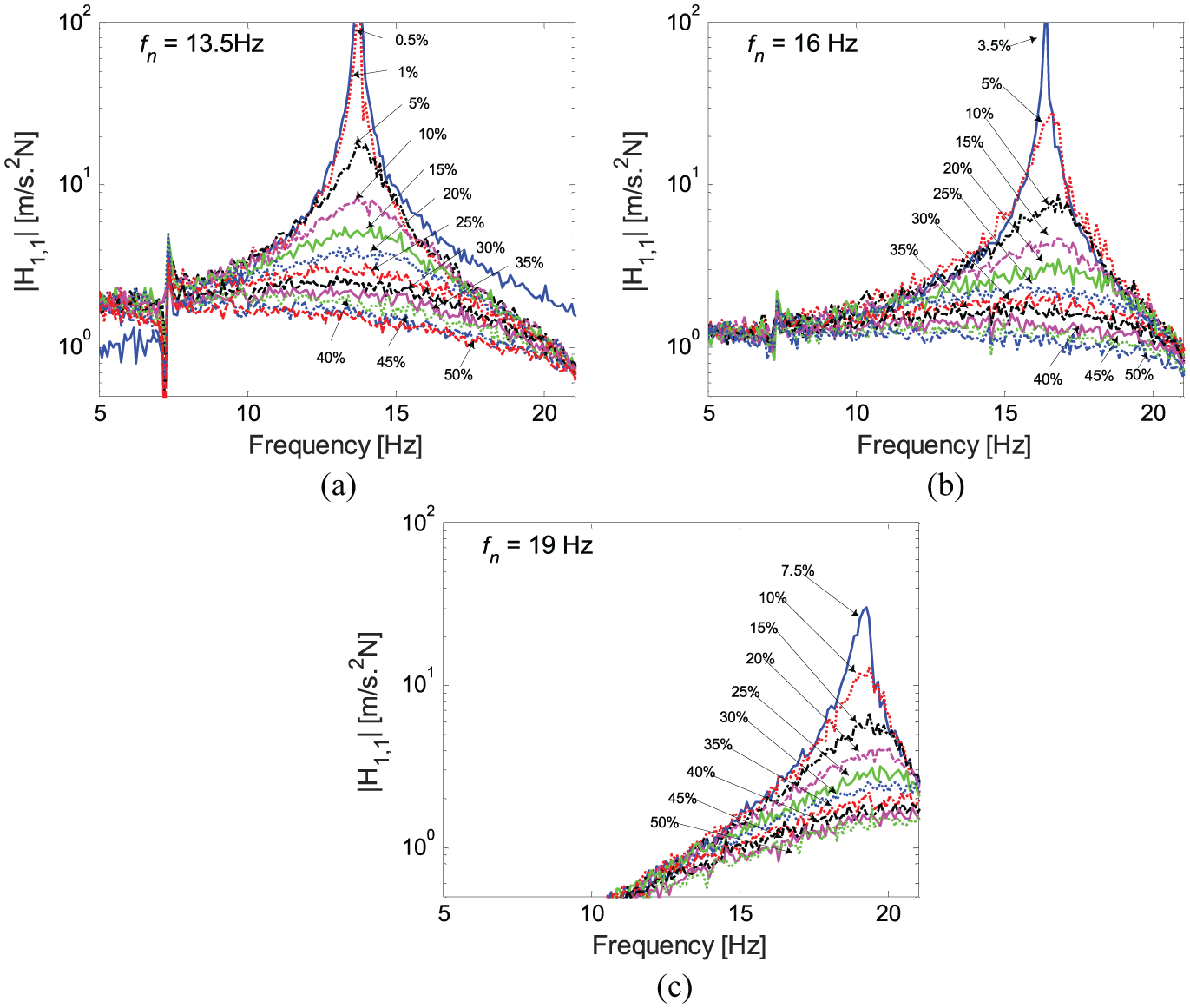
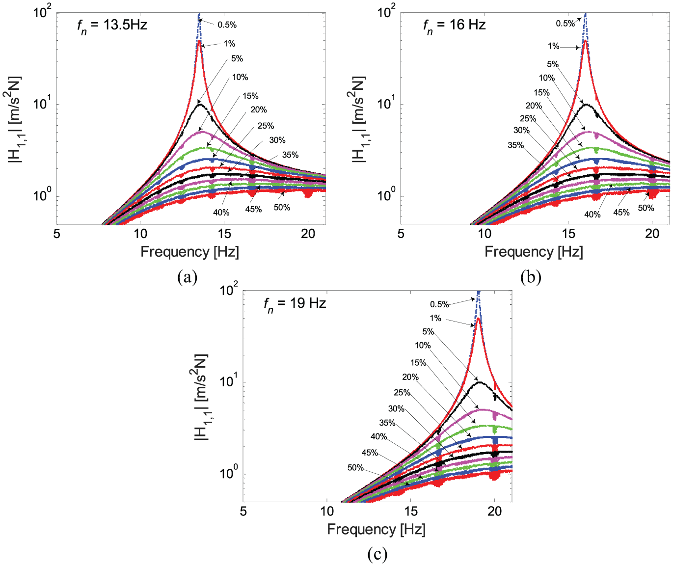
Experimental closed-loop FRFs.
Numerical closed-loop FRFs.
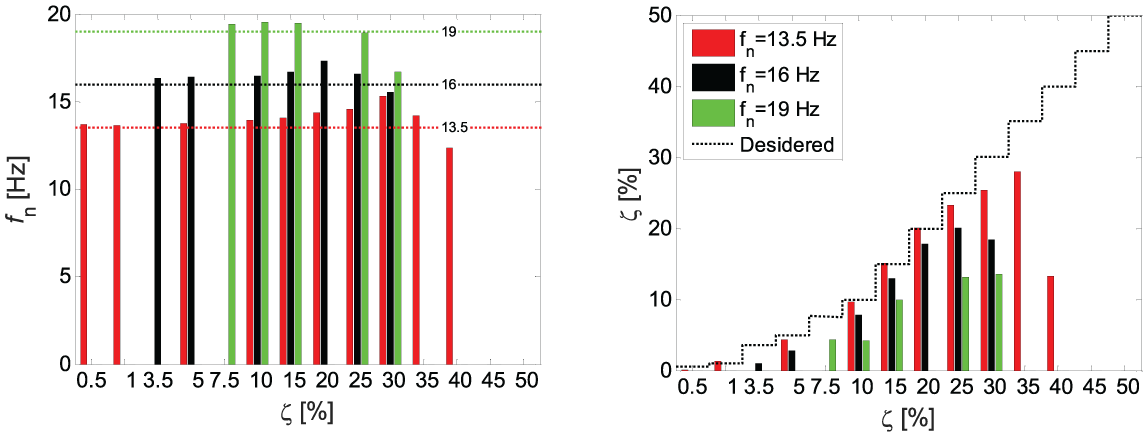
The natural frequencies and damping ratios of the closed-loop system are compared to assigned values in Figure 13. The poles are correctly identified until ζn = 30–35% in the closed-loop FRFs. For very high levels of damping ratio, the identification is no longer feasible, although from the experimental FRFs it is clear that the damping is increasing. Successful assignment of the desired natural frequency through feedback linearisation is possible in almost all the cases in which a pole is identified. When the assigned natural frequency is
Feedback linearisation
Analysing the phases of the linearised degree of freedom, the assigned natural frequencies are located very close to the −90° phase point, as in Figure 14. The slope of the phase decreases with increasing damping ratio, thereby confirming the expected increased damping.
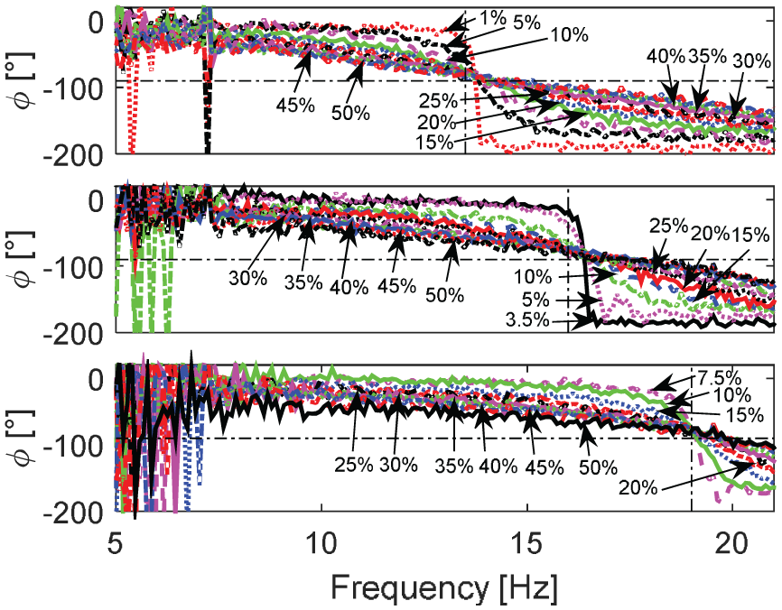
Experimental closed-loop FRF phases.
The experimental time domain responses of the controlled (
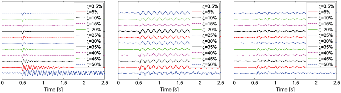
Time domain responses for
Although the first degree of freedom is linearised by the controller, the internal dynamics (second and third degrees of freedom) remains nonlinear. The FRFs pertaining to the third degree of freedom for the various values of natural frequencies and damping ratios assigned to the first (controlled) degree of freedom are shown in Figures 16 and 17 for the numerical and experimental cases, respectively. The expected multi-mode dynamic behaviour is evident from these plots; there are two fixed resonances at natural frequencies corresponding to the first and third open-loop modes, and a third peak corresponding to the dynamics assigned to the first degree of freedom. The clearly visible jump in the numerical simulations of H1,3 is not visible in the experimental results because the FRFs were obtained from hammer tests.
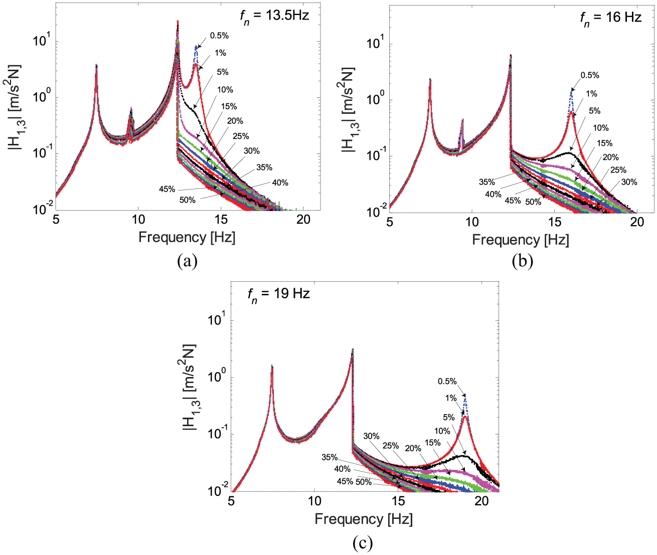
Numerical closed-loop internal dynamics H1,3.
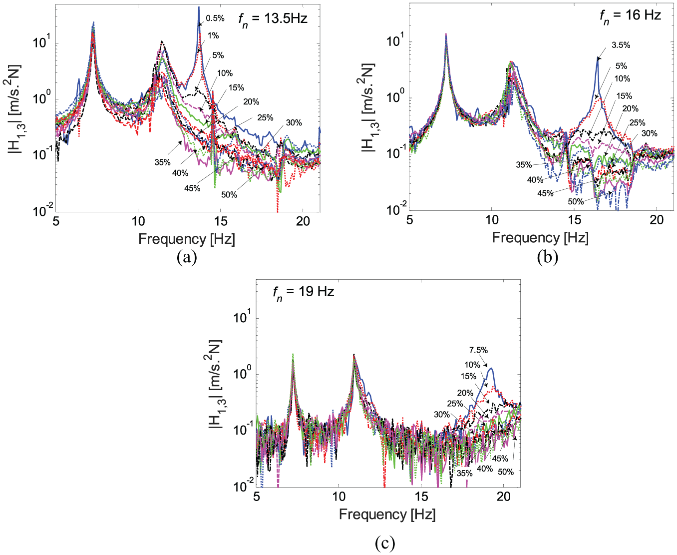
Experimental closed-loop internal dynamics H1,3.
The
7. Conclusion
The application of a new control approach that combines partial feedback linearisation with the receptance method, previously studied theoretically and in simulation, is experimentally investigated in this paper. The new method is able to linearise the system without the necessity of a system model, thereby eliminating errors due to inaccuracies in the numerical representation of the system. The controller is implemented on a three degree of freedom nonlinear system with a piecewise-linear stiffness characteristic. With the input and output at the first degree of freedom, the nonlinearity is located at the third degree of freedom. The control configuration results in the internal dynamics being non-smooth, and its stability is studied using a receptance-based method. Partial feedback linearisation is successfully achieved, with the linearised (first) degree of freedom displaying a single mode at the assigned natural frequency while the other modes are almost completely cancelled out, except for small discrepancies when the assigned natural frequency is low. The agreement between desired and actual values of natural frequencies and damping ratios is very good, except for a few cases when a pole cannot be identified or the shaker saturates.
Footnotes
Appendix
The nonlinear damping force, as given in equation 7, is represented in the F-x plane as shown in Figure 18. The DF is defined as
Because in this case the force is a dissipative force, the cycle is in the counter-clockwise direction.
As this is a non-conservative (dissipative) force, the in phase term is expected to be zero.
Defining the switching point
Applying the definition in equations (28) and separating those regions within the integral when the gaps are either open or closed (so the k2 is active)
Simplifying the regions in which the force is null
The ‘signum’ function may be eliminated by casting the above equation as follows
Computing the integrals, one finds that
The term in quadrature is computed by applying equation (29). Simplifying the region in which the integrand function is zero results in
Eliminating the ‘signum’ function as before
Computing all the integrals, the in-quadrature term becomes
The DF for the nonlinear damping force when
The complete formulation can be written as
where
Acknowledgements
The research described in this paper was carried out during a visit to the University of Liverpool by the first author, Domenico Lisitano.
Funding
Domenico Lisitano wishes to acknowledge support provided by an Erasmus+Traineeship funded by the European Commission.