Sage Journals: Discover world-class research

Abstract

The increasing complexity of driving functions at the overall vehicle level leads to high requirements for validating them. To shorten this process, it is necessary to validate the overall vehicle properties at the hardware level of the subsystem, which becomes a cyberphysical prototype in a hardware-in-the-loop (HiL) environment. With a focus on the longitudinal vehicle shuffle characteristics, the influence of the side shafts and tires is particularly dominant. The latter can be represented by a large number of available tire models, which are known through full-simulative vehicle approaches. However, a comprehensive overview of their use and scientific analysis of the influences on the cyberphysical specimen and the measurement results is lacking. These are fundamental as a basis for enabling validation of the powertrain subsystem. To evaluate this influence of tire models on the cyberphysical specimen on the HiL, various models with different degrees of abstraction are run, with the focus on full vehicle shuffle characteristics. The results show a significant influence of the tire models on the damping behaviour of the oscillation. Increasing slip values results in a higher damping influence of the longitudinal vehicle shuffle. The natural vehicle shuffle frequency is only insignificantly influenced. The impacts on the shuffle align with the findings from the literature, taking into account a real full vehicle. Further investigations are needed to determine the latency of signal transmission between the HiL and vehicle simulation for highly dynamic manoeuvres, aiming to obtain more stable speed signals and thus achieve better quality results.

Keywords

driveability electrical powertrain hardware-in-the-loop vehicle shuffle frequency coupled vehicle simulation

Introduction

The vehicle development process can be described by the V-model, named after its shape, which consists of system design and system integration. At the macro level, the V-model comprises three levels: system, subsystem, and component levels. Property verification and validation are conducted continuously at each stage of the development process. The complexity of the systems increases during the ongoing validation process (Düser, 2010).

Validating an increasing number of driving functions means an increase in the complexity of the validation process (Düser, 2010). By combining a specimen with a (cyber-) physical complete vehicle environment, a system can be created in which the real hardware behaves in the same way as if it were implemented in a real vehicle. The results of the device under test (DUT) directly influence the calculations of the coupled simulation. This approach is generally referred to as hardware-in-the-loop. The result of the test rig is strongly dependent on the test rig itself, the DUT, the degree of abstraction of the coupled simulations, and their real-time capability (Andert et al., 2018; dos Santos et al., 2018; Brayanov and Stoynova, 2019).

Depending on which driving function or vehicle characteristic is to be analysed, different challenges arise for the validation process. One characteristic vehicle property is longitudinal vehicle body oscillation, also known as longitudinal vehicle shuffle. This phenomenon is due to the first natural frequency of the powertrain and can be perceived as unpleasant by the occupants, making it an important factor in driving comfort. (Fan, 1994).

Oscillations up to 30 Hz can be categorised as relevant for driveability. Humans perceive frequencies up to 10–12 Hz as particularly unpleasant, due to their perception of vibrations. The frequency range collides with the longitudinal vibration of the vehicle, emphasising the importance of driveability tests (Schmidt et al., 2023; Verein Deutscher Ingenieure, 2017).

The literature research in Hübner and Prokop (2025) shows that the validation of the overall vehicle characteristic of longitudinal vehicle shuffle frequency is not yet being carried out at the subsystem level. The significant influence of the side shafts and tire properties on the position and vibration behaviour of the longitudinal vehicle shuffle is known from the literature, primarily referring to results from simulations or tests with complete vehicles or powertrains with real tire-road contact (Fan, 1994; Figel et al., 2019; Hülsmann, 2007; Lukac et al., 2016; Pillas, 2017; Sorniotti, 2008). The side shafts essentially influence the frequency, and the tire slip influences the damping behaviour. A significant analysis of this correlation using a HiL with the DUT and coupled full vehicle simulation, including tire-road contact, is missing. These are fundamental as a basis to enable driveability validation on the powertrain subsystem.

Since the real side shafts are used in this test rig application, their influence is recorded and taken as given. However, the road contact and the coupled simulation models represent slip. The influence of the tire model abstraction on the resulting longitudinal vehicle acceleration is to be investigated.

Therefore, this article will examine the influence of different known commercial tire models on the longitudinal vehicle shuffle to address the following questions:

- How do the vibrations affect the cyberphysical system, and can the tire models be used at the user level?

- What influence does the tire simulation of the coupled vehicle simulation (tire-road contact, vibration behaviour) have on the virtual longitudinal vehicle shuffle?

This article is organised as follows: first, the mechanism behind vehicle shuffling and different tire models is shown. In the next step, the test rig used for the investigations and the manoeuvres performed are presented. In the following, the measurements are analysed and the results are presented. Finally, a conclusion is drawn regarding the influence of tire models on the cyberphysical specimen and vehicle shuffle, as well as the challenges that still exist for the application in HiL.

Tire models

Many common tire models can be integrated into CarMaker. For example, these models can feature a flexible tire belt, allowing them to map more complex tire modes and thus higher frequency ranges (FTire). Due to their high complexity, these tire models also result in higher demands on computing time, and therefore, a real-time capability is required. That’s the reason why FTire is only available in CarMaker Office and not in CarMaker Testbed for HiL applications (IPG Automotive GmbH, 2023b).

Coupling individual tire models is also feasible and should therefore be considered, depending on the application.

In addition, the model used must always be based on consistent and valid parameters to generate plausible and transferable results. As the complexity of the tire model increases, so do the demands on the parameterisation method and, consequently, the costs.

With a focus on real-time capability and the frequency range of driveability to be considered, IPG CarMaker’s tire model ‘RealTime Tire’ and the very common MF-Tyre, respectively. MF-SWIFT model are considered. The main theoretical principles underlying the selected tire models are presented below.

RealTime Tire

The RealTime Tire model is the real-time version of the IPGTire model and the default tire model in CarMaker. It is based on tire measurements:

- Longitudinal force (F_x) and slip (s) $\to F_{x} = f u n c t i o n (F_{z}, s)$

- Lateral force (F_y) and slip angle (α) $\to F_{y} = f u n c t i o n (F_{z}, α)$

- Self-aligning torque (M_z) and slip angle $\to M_{z} = f u n c t i o n (F_{z}, α)$

and is therefore an empirical model. The tire measurement data points are approximated using CarMaker through a combination of exponential and cubic splines, which provides flexibility for the input data. During simulation, this interpolated function is used (IPG Automotive GmbH, 2023a).

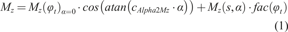
The RealTime tire also takes into account a standstill mode and the relaxation length, whereby the parking torque in a standstill is described as follows:

M_{z} = M_{z} {(φ_{t})}_{α = 0} \cdot c o s (a t a n (c_{Alpha2Mz} \cdot α)) + M_{z} (s, α) \cdot f a c (φ_{t})

(1)

with φ_t as the turn slip and c_Alpha2Mz as a decline coefficient of the pure turn slip aligning torque, depending on the side slip angle. The factory settings can be optionally adjusted. (IPG Automotive GmbH, 2023a; 2023b)

MF-Tyre

The semi-empirical Magic Formula (MF-Tyre) tire model is a widely used method for calculating tire forces and torques in static and quasi-static applications (Pacejka, 2012).

The input and output behaviour of the wheel-road contact is described purely mathematically. The aim is to analytically link the lateral forces, the circumferential forces, and the self-aligning torques with the tire slip. To this end, these relationships are first measured and then approximated using mathematical functions. (Schramm et al., 2013).

The general equation of the Magic Formula is defined in Pacejka (2012) for given wheel loads and camber angles:

\begin{align} y & = D \cdot s i n (C \cdot a r c t a n (B x - E \cdot (B x - a r c t a n (B x))) \end{align}

(2)

\begin{align} Y (X) & = y (x) + S_{V} and x = X + S_{H} \end{align}

(3)

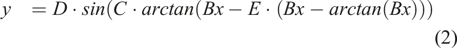
The variables used are defined as follows, according to Pacejka:

- Y describes either the longitudinal force F_x or the lateral force F_y or the aligning torque M_z,

- X describes either the longitudinal slip s or the slip angle α,

- B is a stiffness factor, C is a shape factor, D is the maximum value, E is a curvature factor, and S_V or S_H are vertical or horizontal displacements concerning the zero crossing of the curve.

Further information on determining the influencing factors and their effects on the characteristic curve can be found in Pacejka (2012).

MF-SWIFT

The structure of the short wavelength intermediate frequency tire (SWIFT) model is shown in Figure 1 and can be divided into five parts according to Pacejka (2012):

(1) The mechanical replacement model of the tire, whereby a rigid ring replaces the inertia of the tire belt. It describes the tire dynamics up to approximately 60 Hz.

(2) The residual stiffnesses in longitudinal, lateral, vertical and yaw direction, which must be introduced to describe the overall static stiffnesses of the tire and to capture the vibration capacity of the belt. They are placed between the ring and the road surface. The overall stiffness consists of the partial stiffnesses of the carcass, the tread and the residual stiffness.

(3) The brush model, which represents the contact area and takes into account the running surface compliance and sliding components. This model approximates the contact surface dimension and considers the input wavelengths from 10 cm.

(4) The ground contact model describes the enveloping behaviour of the tire on the uneven, three-dimensional road surface using the following parameters: the effective tread height, the effective forward and lateral inclination of the road surface and the effective road curvature, which influences the effective rolling radius.

(5) The MF-Tyre model is used to calculate non-linear slip forces and torques.

Overall, the SWIFT model can be divided into three submodels: the slip model, the vibration model, and the ground contact model. According to Pacejka, the range of validity must be limited to wavelengths of approximately 10 cm or smaller, individual obstacles, excitation frequencies below 80 Hz, and large slip states.

Figure 1.

Schematic representation of the SWIFT model with two translational and one rotational spring-damper element according to Zegelaar (1998).

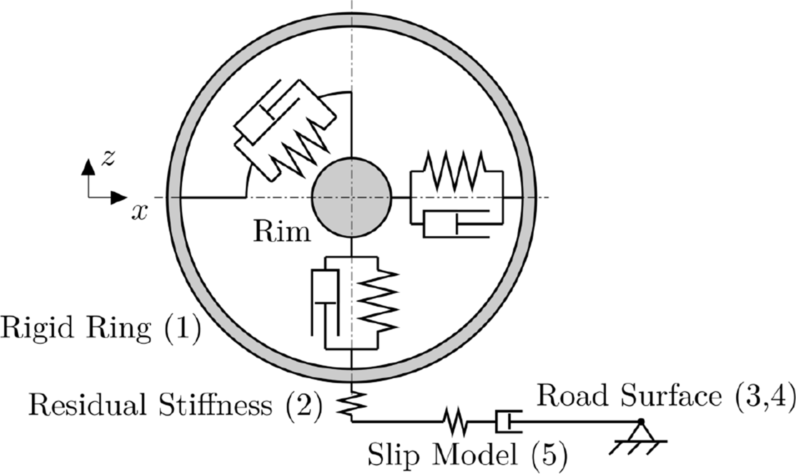
The ground contact model of the SWIFT model serves as a low-pass filter for unevenness in the road surface. This geometric filtering describes the enveloping behaviour of small obstacles and takes place in the contact area. According to Pacejka, a slow pass over small obstacles results in changes in both longitudinal and vertical forces, as well as a change in angular velocity, due to a change in the rolling radius. The radius increases briefly when the tire hits the obstacle due to tire inertia (Pacejka, 2012). Due to ideal, flat road surfaces, the ground contact model will not be considered in more detail in the following section.

HiL application for driveability investigation

HiL setup

Figure 2 shows the schematic structure of the test rig used. An electrical drive unit (EDU), consisting of an inverter, motor control unit, permanent magnet synchronous machine, gear stages and side shafts, represents the DUT. The power supply is provided by a battery emulator, which replaces the vehicle battery. The CAN communication between the test rig and EDU runs at 100 Hz, which only affects the torque demand signal. The load machines are each supplied and controlled by a frequency converter, which enables operation in four quadrants.

Figure 2.

Powertrain test bed with applied electrical drive unit and coupled full vehicle simulation (Hübner and Prokop, 2025).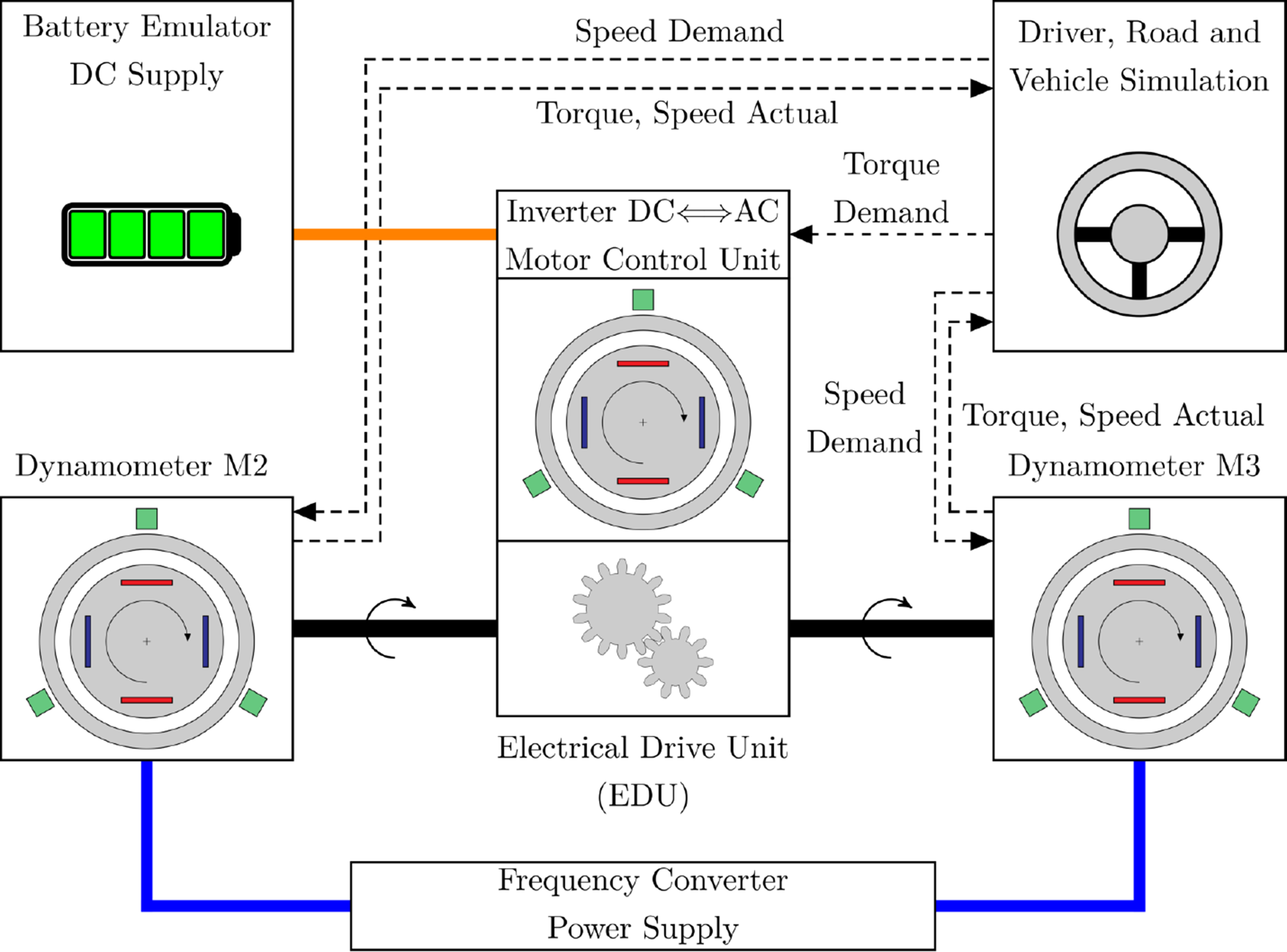

The coupled overall vehicle simulation is executed on a real-time computer and connected to the test rig at a rate of 1 kHz via User Datagram Protocol (UDP). It is the default transmission frequency set by IPG and is therefore considered a given for the user initially. Depending on the manoeuvre or the frequency range under consideration, the mapping quality of possible phenomena by the transmission frequency must be checked. There are various regulations on the ratio of transmission frequency to event frequency to avoid aliasing, at least a factor of 2 to greater than 20 is recommended (Lunze, 2020). With a given transmission rate of 1 ms, frequencies of at least 50 Hz can therefore be transmitted. Focusing on vibration phenomena of driveability (Schmidt et al., 2023) and the rigid ring modes of tires, this frequency range can be considered sufficient. When examining phenomena such as noise and harshness, flexible tire belt properties, or the influence of electrical engine characteristics like torque ripple, the transmission range must be considered critically.

Note that the load machines are in a closed control loop, while the DUT is only controlled in an open control loop due to the lack of feedback sensors. The main specifications of the test rig are summarised in Table 4.

Tire model settings

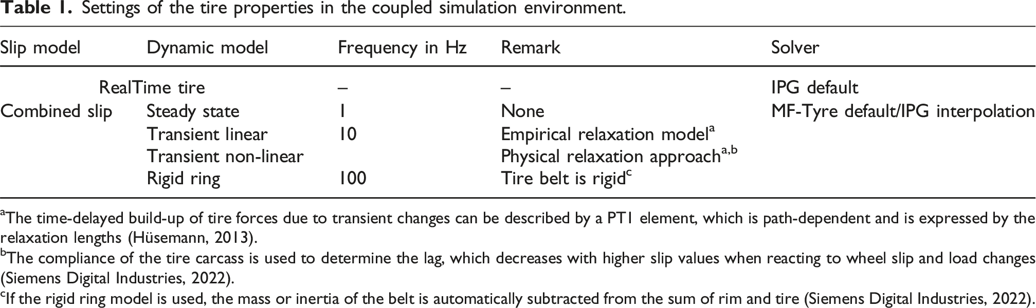
A distinction is made between five variants for the variation of the tire model, which are summarised in Table 1. The dimensions of the tire can be found in Table 4. The CarMaker standard model RealTime Tire is used in the default variant. The SWIFT model can be customised in the tire options in CarMaker. The following properties have been defined and are not varied:

(1) Tire Side: Automatic,

(2) Contact Method: Smooth Road,

(3) Slip Forces: Combined,

(4) Temperature and Velocity: Disabled.

Table 1.

Settings of the tire properties in the coupled simulation environment.

Slip model	Dynamic model	Frequency in Hz	Remark	Solver
RealTime tire		–	–	IPG default
Combined slip	Steady state	1	None	MF-Tyre default/IPG interpolation
	Transient linear	10	Empirical relaxation model^a
	Transient non-linear	10	Physical relaxation approach^a,b
	Rigid ring	100	Tire belt is rigid^c

^aThe time-delayed build-up of tire forces due to transient changes can be described by a PT1 element, which is path-dependent and is expressed by the relaxation lengths (Hüsemann, 2013).

^bThe compliance of the tire carcass is used to determine the lag, which decreases with higher slip values when reacting to wheel slip and load changes (Siemens Digital Industries, 2022).

^cIf the rigid ring model is used, the mass or inertia of the belt is automatically subtracted from the sum of rim and tire (Siemens Digital Industries, 2022).

Regarding the slip model, several calculation options are available for selection. In terms of use on a HiL and the safety of the EDU, the following options are considered unsuitable:

- MF-Tyre is deactivated, there are no slip forces (only F_z) and therefore no force transmission. The tires or load machines are accelerated, as the EDU provides torque to achieve the required vehicle velocity, but the vehicle does not move. The load machines drive up to the speed limit of the EDU, and an emergency shutdown of the HiL system occurs, along with deactivation of the connection between the simulation and test rig.

- Only longitudinal slip forces and torques are calculated. The required velocity can be adjusted accordingly, and then the virtual vehicle drives. Due to oscillation in the speed and torque signals of the load machines, the longitudinal forces in the vehicle simulation are not identical at the rear axle, resulting in a yaw moment. As no lateral forces are calculated, the yaw movement cannot be compensated, and the vehicle drives off the carriageway, resulting in the simulation being cancelled and the HiL going to idle.

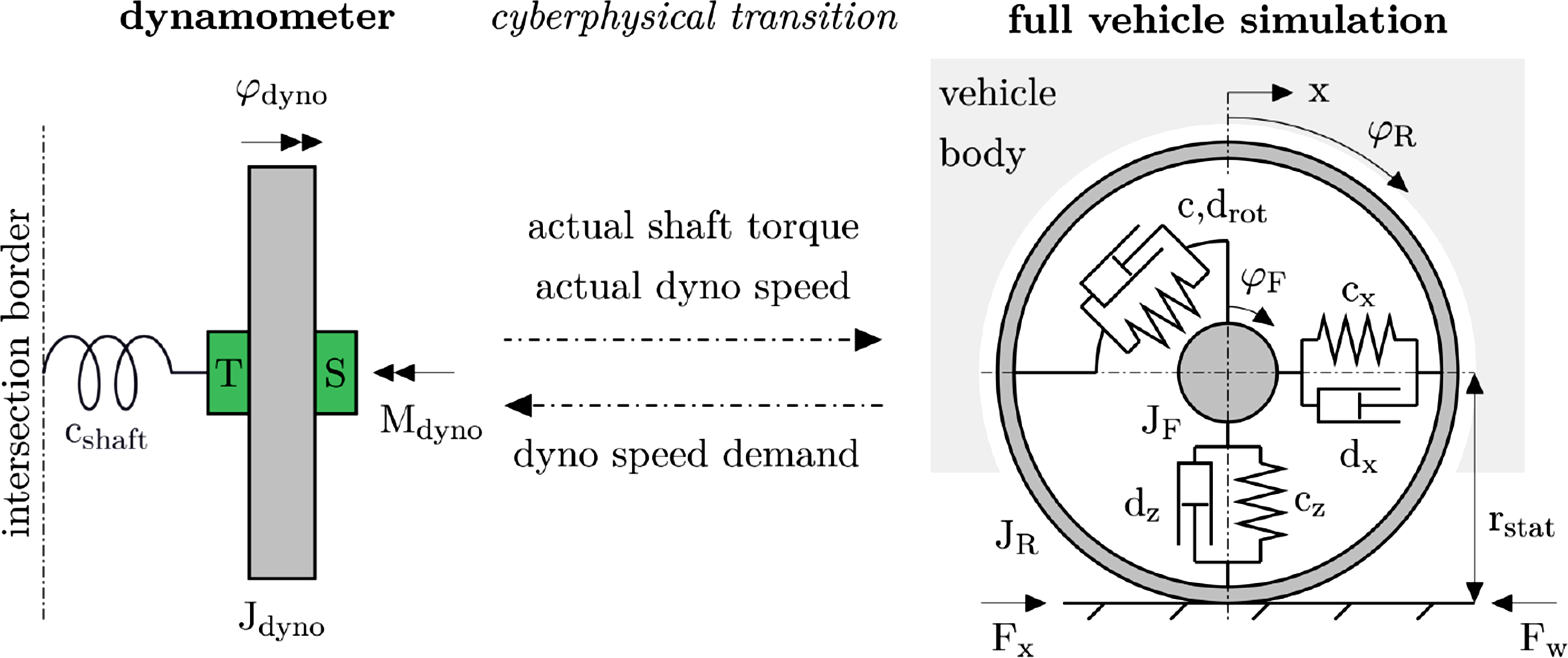
The use of the combined slip model with the calculation of F_x,y,z and M_x,y,z is therefore preferable for the application (IPG Automotive GmbH, 2023b). As shown in Table 1, the solver of the MF-SWIFT model can also be customised. The default solver calculates with a step rate of 1 kHz and passes on the last result, if queried with a higher frequency, until the next calculation step (Siemens Digital Industries, 2022).The relationship between physical load machine/virtual wheel speed and longitudinal acceleration of the virtual vehicle body can be explained in a simplified way, neglecting the influence of the rotating translational dampers. Using the representation in Figure 3, the equations of motion can be found in equations (4)–(8) (cf. (Fan, 1994)), taking into account the slip definition:

\begin{align} F_{x} \cdot r_{stat} & = F_{w} \cdot r_{stat} + m_{vehicle} \cdot \ddot{x} \cdot r_{stat} \end{align}

(4)

\begin{align} F_{x} \cdot r_{stat} & = J_{R} \cdot {\ddot{φ}}_{R} + F_{w} \cdot r_{stat} + c_{rot} (φ_{R} - φ_{F}) + d_{rot} ({\dot{φ}}_{R} - {\dot{φ}}_{F}) \end{align}

(5)

\begin{align} M_{shaft,virt} & = J_{F} \cdot {\ddot{φ}}_{F} + c (φ_{F} - φ_{R}) + d_{rot} ({\dot{φ}}_{F} - {\dot{φ}}_{R}) \end{align}

(6)

\begin{align} \ddot{x} & = {\dot{ω}}_{tire} \cdot r_{dyn} \cdot (1 - s) \end{align}

(7)

Figure 3.

Transition of cyberphysical system with a dynamometer (Sensors for speed (S) and torque (T) in green) and the coupled full vehicle simulation with tire-road-contact, simplified illustration.

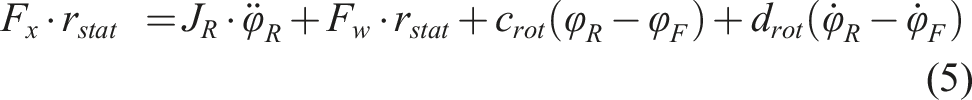
The equation for the simplified model of the load machine on the test rig side is as follows:

M_{shaft,real} = J_{dyno} \cdot {\ddot{φ}}_{dyno} + M_{dyno}

(8)

With F_x as the driving tire force, r_stat,dyn as the static or dynamic tire radius, F_w as the force of the driving resistances (air, gradient and rolling resistance), m_vehicle as the vehicle body mass, x as the translational coordinate in the longitudinal direction of the car, ω_tire as the tire angular velocity, s as longitudinal slip, c_{rot, shaft} as the rotational stiffness and d_rot as damping coefficient. The torque transmitted from the real EDU via the side shaft to the test rig load machine is labelled M_{shaft, real}, and the equivalent torque taken into account for the simulation is labelled M_{shaft, virt}.

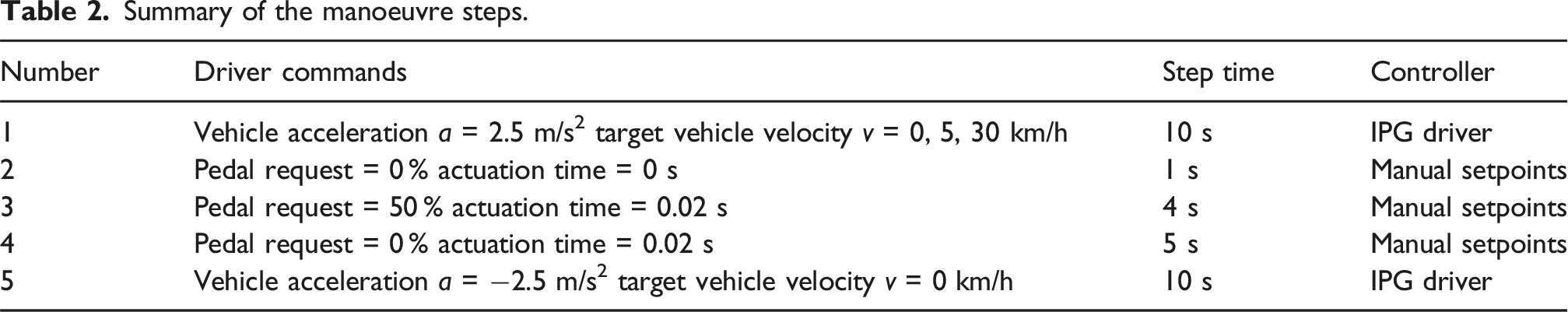
Manoeuvre definition

A step function in the setpoint specification is suitable for characterising the first natural frequency of the powertrain in the HiL system. It allows conclusions to be drawn about the step response, the frequency response, and the first torsional natural frequency (Schmidt and Prokop, 2023).

To analyse the significant characteristics of driveability, the following manoeuvres are specified in the CarMaker Testbed environment and are listed in Table 2. Each manoeuvre is performed once on a dry road and once on a wet road (μ = 1, resp. 0.5) and driven three times; the total number of measurements is 90. With the specification of the coefficient of friction, the transmissible longitudinal and lateral force also changes, taking into account the wheel contact force, resulting in different slip curves.

Table 2.

Summary of the manoeuvre steps.

Number	Driver commands	Step time	Controller
1	Vehicle acceleration a = 2.5 m/s² target vehicle velocity v = 0, 5, 30 km/h	10 s	IPG driver
2	Pedal request = 0 % actuation time = 0 s	1 s	Manual setpoints
3	Pedal request = 50 % actuation time = 0.02 s	4 s	Manual setpoints
4	Pedal request = 0 % actuation time = 0.02 s	5 s	Manual setpoints
5	Vehicle acceleration a = −2.5 m/s² target vehicle velocity v = 0 km/h	10 s	IPG driver

Analysis of measurements

Solver analysing

The Default MF-Solver leads to oscillations in the speed signal, which occur particularly with the transient linear and rigid ring dynamic models. This phenomenon is particularly significant at low velocities and during initialisation. Figure 4 shows the speed demands and measured feedback values for the operating point with v = 5 km/h. In the demand values shown, the frequency of the speed signal of the transient linear model is 9–12 Hz and that of the rigid ring is 21–23 Hz. The frequencies in the measured variables are at 9–12 Hz, respectively. It is therefore below the critical transmission frequency and does not show any significant deviation when comparing the default and actual frequency. The latency from the signal transmission (1 ms for one direction) also acts as a dead time and therefore has an unstable effect on the control loop. This latency results in a phase shift in the transfer function, as evident in the speed signals. Overclocking the connection frequency could mitigate this effect and should be investigated in further studies, as shown in Table 4.

Figure 4.

Speed demand signals (above) and measured signals (below) of a load machine for constant vehicle velocity demand (5 km/h) with Default MF-Solver.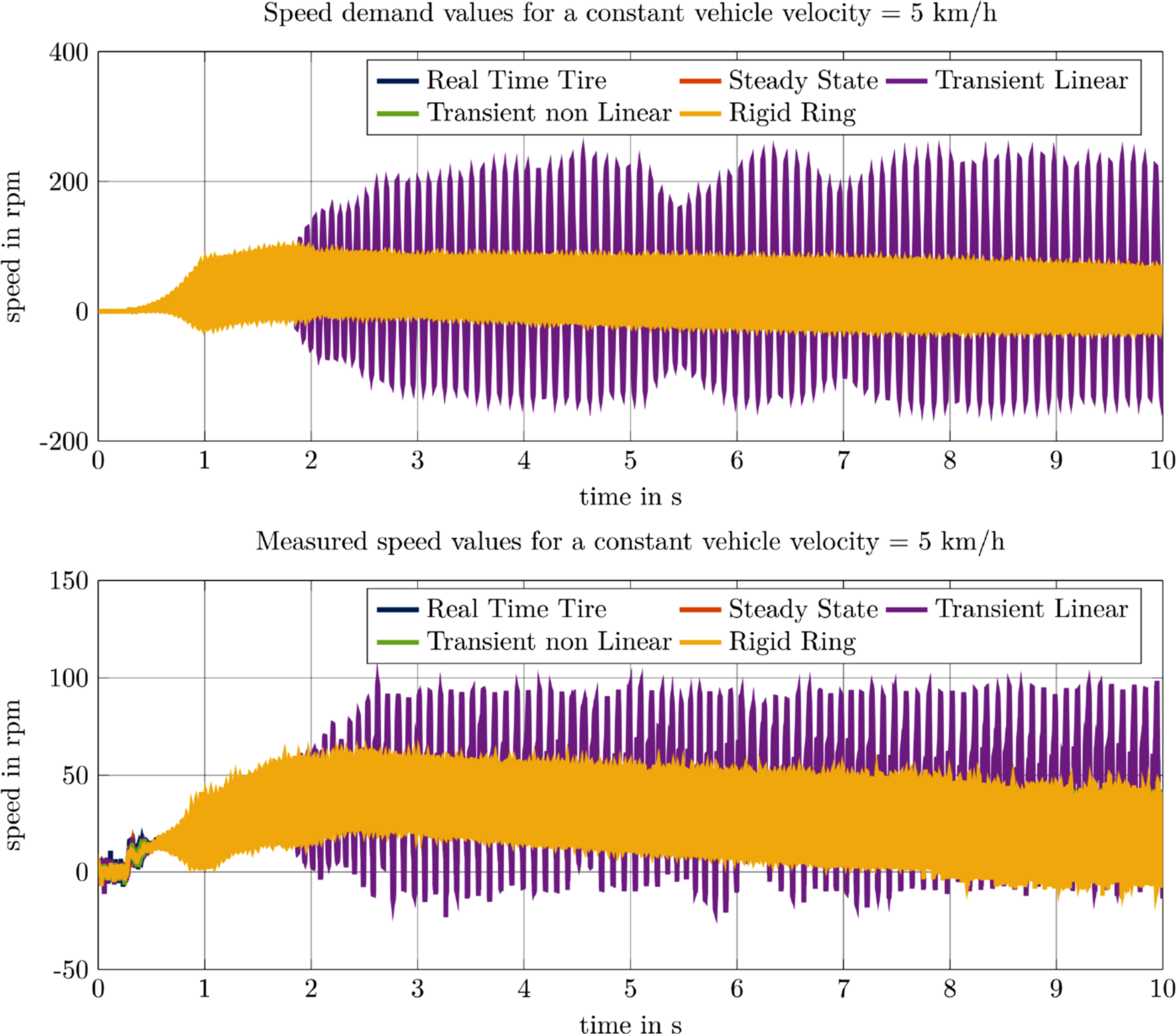

Additionally, for the transient linear SWIFT model, the steady-state operating point with v = 5 km/h cannot be driven, as the EDU oscillates so strongly that the test rig triggers a shutdown. The SWIFT model can therefore not be used safely when utilising tire dynamic properties with the default solver in the application. The same manoeuvre from Figure 4 is driven with the CarMaker solver and shown in Figure 5. The illustration shows a significantly better result for the speed signals, especially for the rigid ring model. The oscillations during initialisation have also been eliminated.

Figure 5.

Speed demand signals (above) and measured signals (below) of a load machine for constant vehicle velocity demand (5 km/h) with IPG-Solver.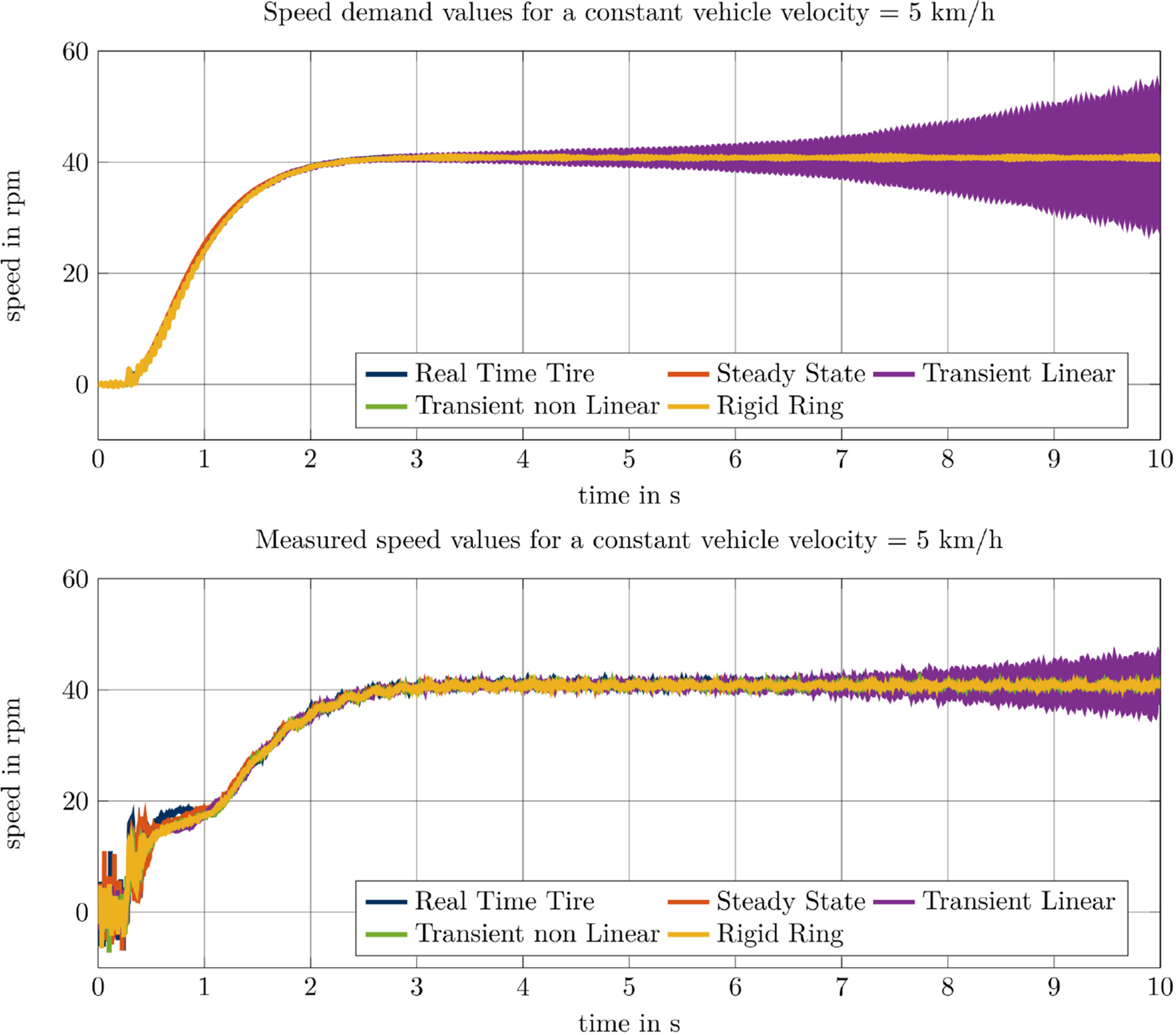

The transient linear dynamic model is still characterised by decaying oscillations, which lie at approximately 20 Hz and must be taken into account for further analyses.

The time-delayed build-up of tire forces, as a result of transient changes (Table 1), is realised as a low-pass filter for the transient linear dynamic model. This transfer function can be sensitive in the case of the given transmission time, respectively transport delay, which can be interpreted as a dead time and therefore causes an instability in the control loop. Due to its location in the software backend, accessibility at the user level is not provided. Possible approaches for analysing this phenomenon will be discussed later on.

Despite this phenomenon, all manoeuvres can be performed with the CarMaker solver (with oversampling, integration substeps: 10), which is used for the following explanations.

Pedal jump

\begin{align} Λ & = \frac{1}{n} \ln |\frac{a (t_{1})}{a (t_{1} + n \cdot T)}|, \end{align}

(9)

\begin{align} D & = \frac{Λ}{\sqrt{{(2 π)}^{2} + Λ^{2}}} \end{align}

(10)

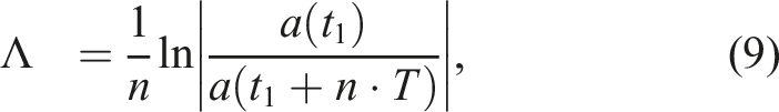
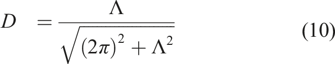
Figure 6 shows an example of one of the manoeuvres with an initial velocity of v = 30 km/h and a friction coefficient of μ = 1. The upper diagram shows the course of the gas pedal position, with the tip-in occurring at t = 11 s. Due to the communication frequency of 100 Hz to the EDU, the signal deviates from the ideal line. The longitudinal acceleration curve of a virtual sensor on the seat rail is plotted in the middle diagram. The bottom plot displays the longitudinal tire slip curves for each tire model. It should be noted that the maximum slip value for the transient (linear and non-linear), respectively, rigid ring model reaches non-linear slip ranges. In contrast, the RealTime Tire and the steady state model show small values. In particular, the signals of the transient linear and rigid ring tire model are characterised by oscillations. In the following, the frequency and damping (D, see equation (10) with logarithmic decrement Λ) of the longitudinal vehicle shuffle will be analysed. The results are noted in Table 3 and Figure 7. The frequency range of driveability phenomena is at frequencies below 30 Hz (Schmidt et al., 2023), which is why this range is focused on the first natural frequency of the powertrain. As already mentioned, the oscillations for the transient linear and rigid ring models are below 30 Hz. Therefore, this disturbance must be filtered directly to conclude the low-frequency vehicle shuffle. For this purpose, the frequency ranges of the harmonics are first identified and then isolated.

Figure 6.

Tip-in of the cyberphysical vehicle (CarMaker Testbed) – characteristics of the coupled vehicle simulation depending on the tire model, initial velocity v = 30 km/h, μ = 1.

Table 3.

Mean frequency f_mean and damping factor D_mean values (with standard deviation) of the longitudinal vehicle shuffle depending on the tire model.

Value	RealTime	SteadyState	TransientLinear	TransientNonLinear	RigidRing
μ = 1
f_mean in Hz	8.9	8.9	9.1^a	8.5	9.1^a
σ_f in Hz	0.23	0.29	0.16	0.20	0.21
D_mean in -	0.007	0.007	–	0.022	–
σ_D in -	0.0029	0.0019	–	0.0034	–
μ = 0.5
f_mean in Hz	9.3	9.1	9.0^a	8.8	9.0^a
σ_f in Hz	0.43	0.18	0.25	0.35	0.23
D_mean in -	0.008	0.006	–	0.018	–
σ_D in -	0.0030	0.0028	–	0.0052	–

^aA low-pass filter is applied to the data to dampen superimposed oscillations.

Figure 7.

Frequency and damping values (with standard deviation) of the longitudinal vehicle shuffle depending on the tire model.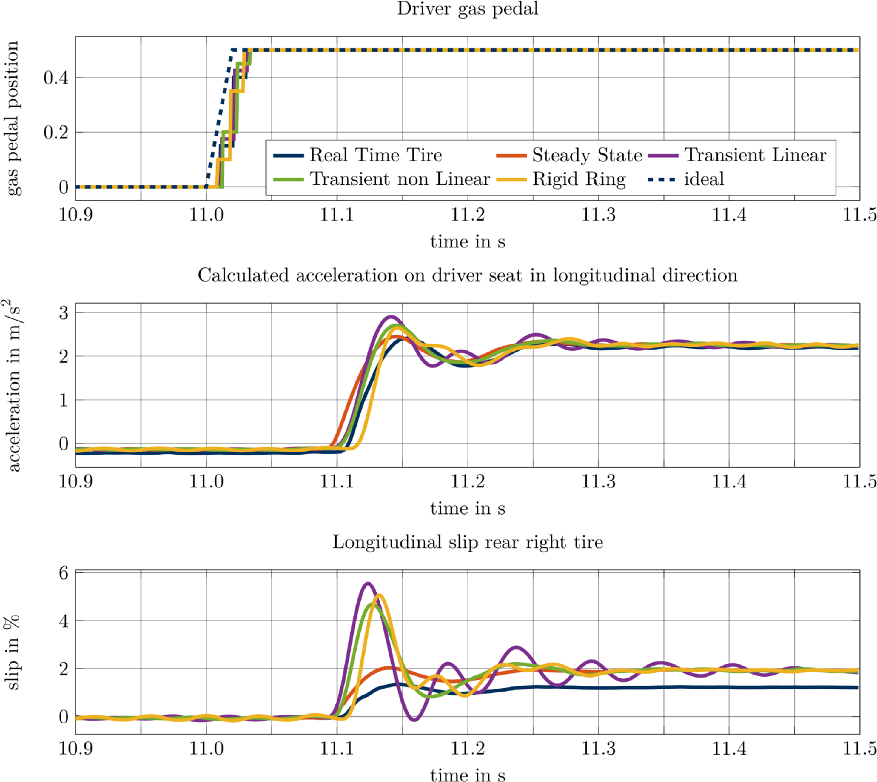

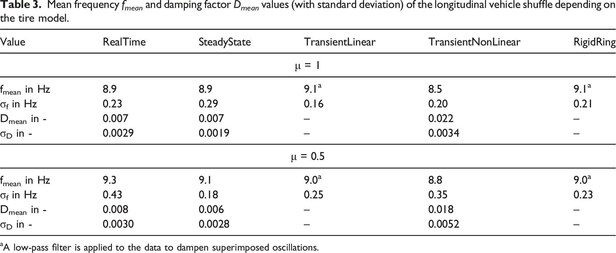
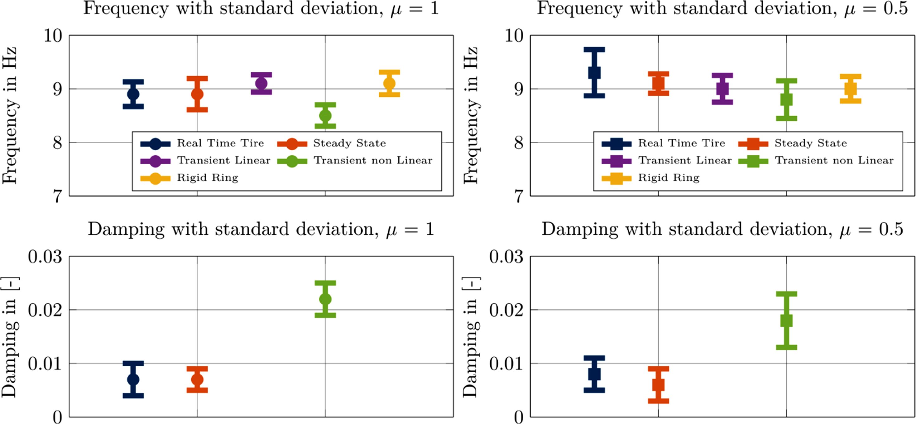
The results in Table 3 indicate a small influence of the tire models on the natural frequency, considering the standard deviation. This finding is consistent with the literature, which indicates that the side shafts, which remained unchanged in this investigation, have a significant influence on the frequency position. The torsional stiffness of the tire (as shown in the rigid ring model) has a subordinate influence due to its larger dimension.

The damping ratio of the tire models (D <1) indicates subcritical damping, which enables the periodic movement shown (Dresig and Holzweißig, 2016). For the tire models investigated, the damping increases with their complexity or with the underlying slip mechanism. This result is consistent with the literature, in which Pillas (2017) describes the slip as the main damping factor. Due to the presence of harmonics, the evaluation of damping in the transient linear and rigid ring model is inconsistent and can therefore not be taken into account. Although the use of a filter provides information on the fundamental frequency, it distorts the damping properties, rendering this approach non-methodical.

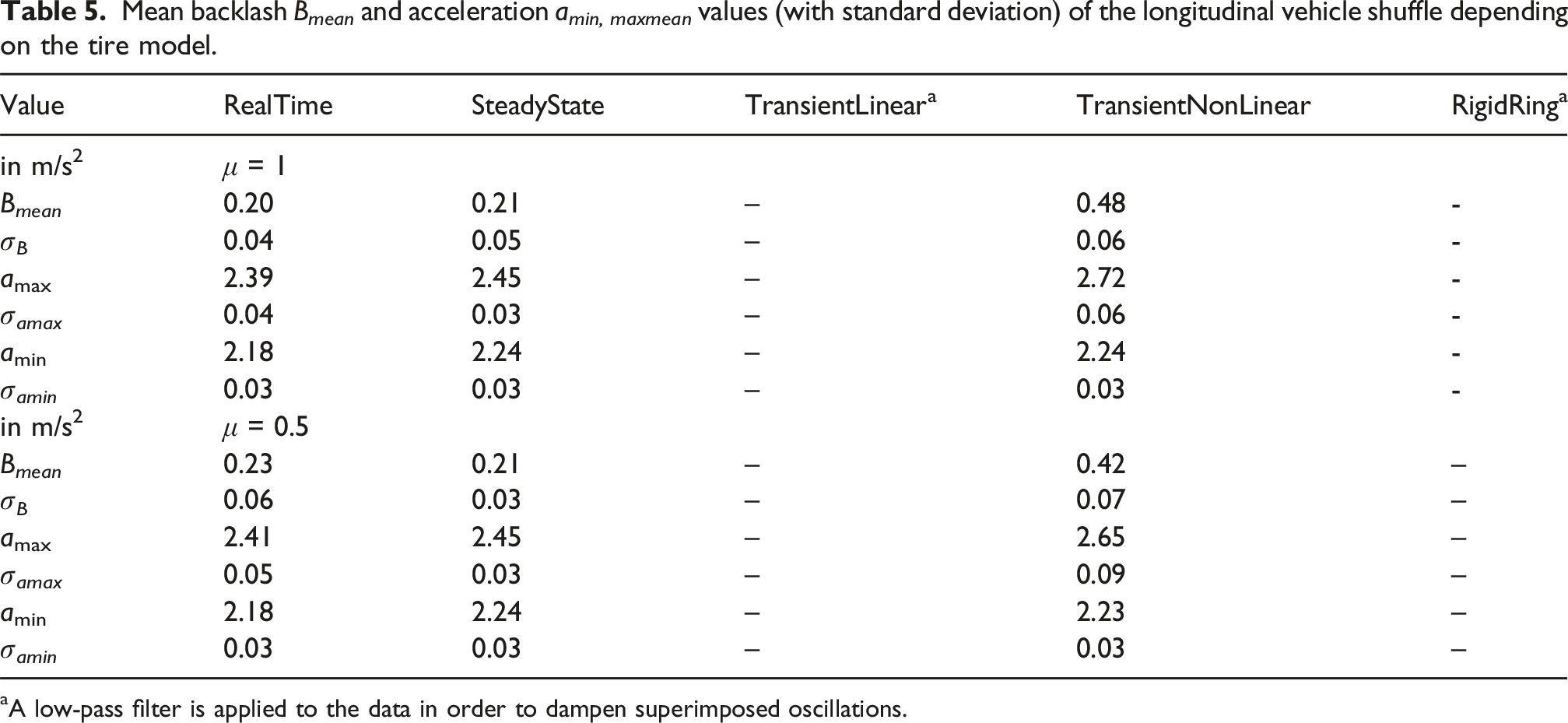
Table 5 shows the results for backlash respectively the maximum and minimum values of the oscillation (Figure 8). Depending on the tire model, the maximum value and therefore the backlash increase.

Figure 8.

Schematic representation of the variables to be analysed in a decaying oscillation, with T – period and B – backlash.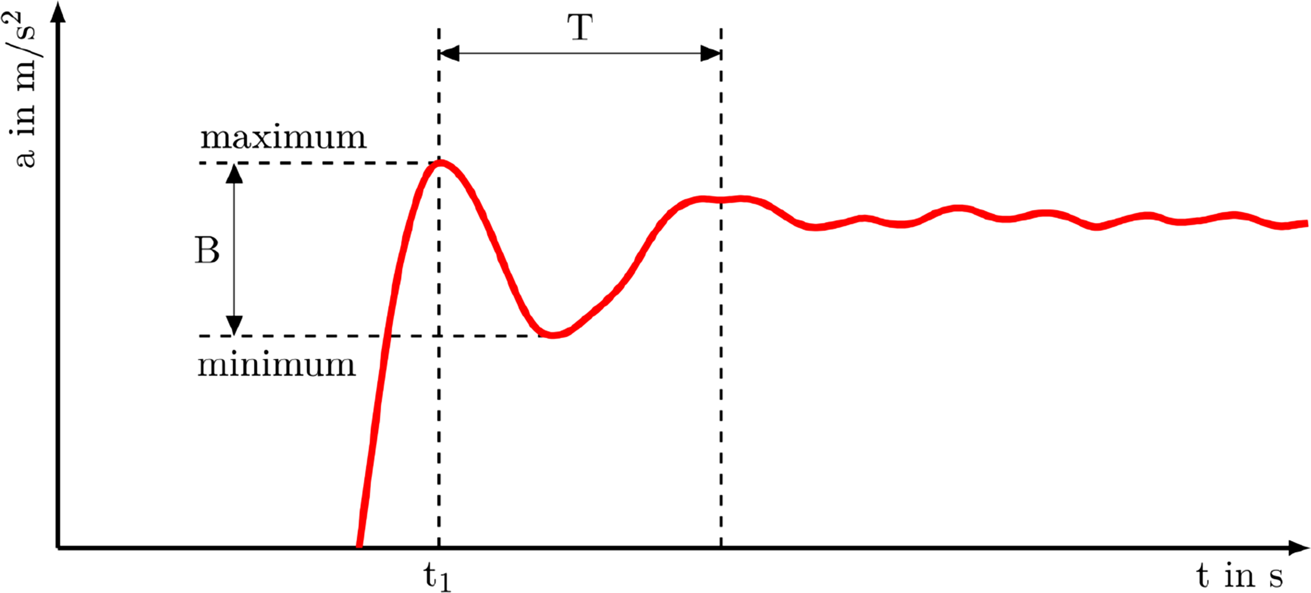

Plausibility check

The influence of the tire model on the vehicle shuffle characteristics can be demonstrated. If the cyberphysical prototype is to be regarded as a basis for validation, it is necessary to consider the plausibility of the results. For this purpose, the slip curves for the three initial velocities are plotted in Figure 9. While slip values of less than 6 % can be seen at v = 30 km/h, high slip values of sometimes more than 20 % can be seen, especially at lower initial velocities.

Figure 9.

Slip curves (vehicle simulation) and actual speed signals (dynamometer) for tip-in manoeuvre, μ = 1.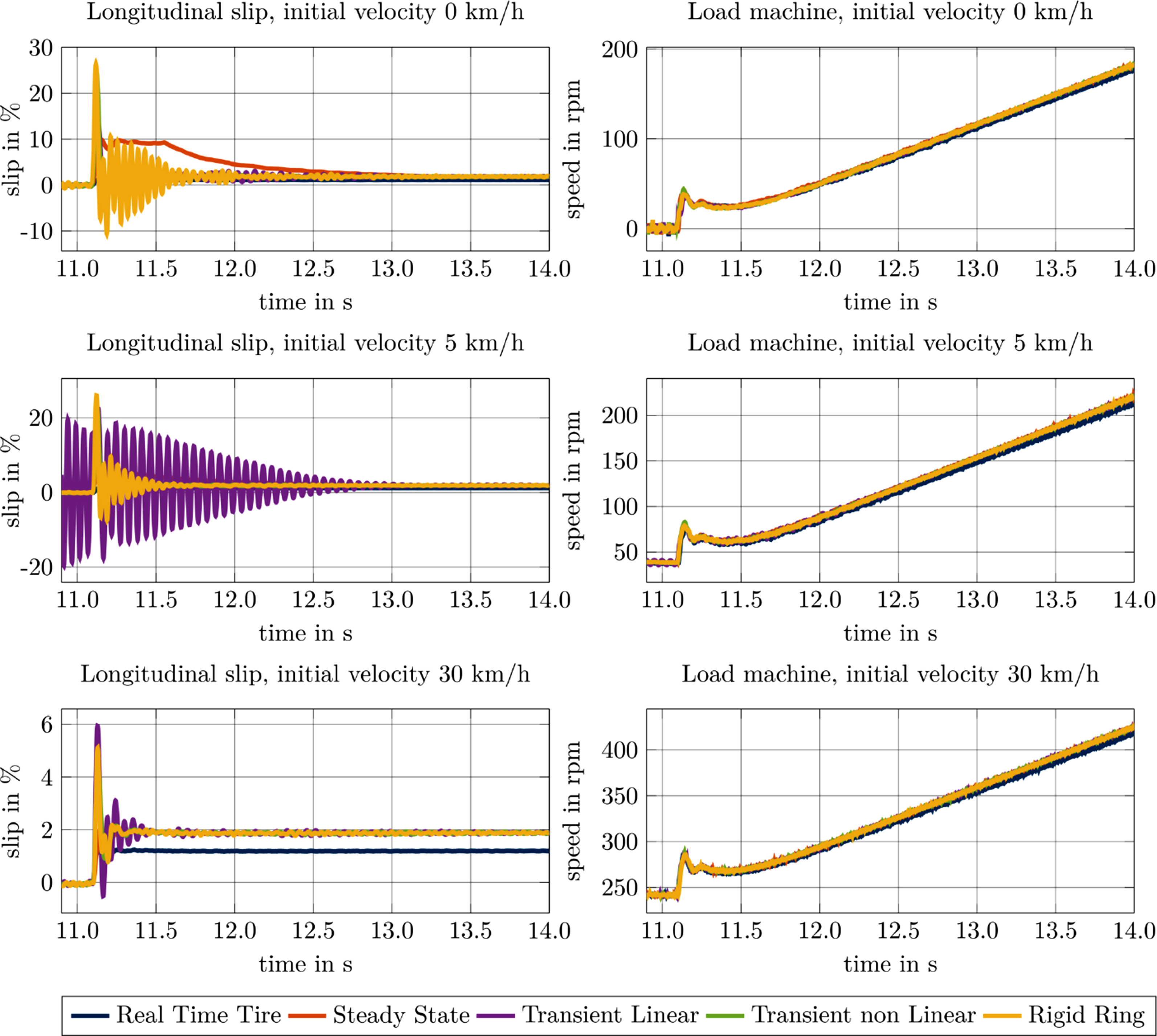

Looking at the fundamental tire properties, the maximal transferable horizontal force is limited by the frictional force, expressed by μF_z, with F_z as the wheel load force. This force includes both longitudinal forces (driving or braking) and lateral forces. The connection is defined via the ’Circle of Forces’: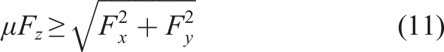

μ F_{z} \geq \sqrt{F_{x}^{2} + F_{y}^{2}}

(11)

Examining the longitudinal slip characteristics in detail, the F_x-s-Diagram (cf. (Schramm et al., 2013)) provides a unified representation. The maximum longitudinal force is limited through μF_z and characterised by the critical slip. When the critical slip is reached, assuming a pure longitudinal manoeuvre, the tire’s traction potential is fully exhausted, as shown in equation (11). The tire glides, and an unstable condition occurs.

In comparison, the applied torque through the pedal jump is 50 % of the maximum engine torque. Because of the gear stages, the open differential, and the static tire radius, the applied force per wheel (F_x) is approximately 2400 N, see equation (12). The limiting frictional force is approximately 5200 N per wheel (for μ = 1) → μF_z > F_x. The critical slip of the set of parameters (MF-Tyre) for the wheel load force and the selected filling pressure is approximately 15 %. In conclusion, the high slip values above the critical slip are implausible for the manoeuvre described. The natural frequency can be excited by a jump function, and a certain boost in the system response is to be expected. Just like a decreasing oscillation to a stable point. However, this is not to be expected in relation to the ramps applied in Figure 12, where the slip is small, but characterised by superimposed oscillations.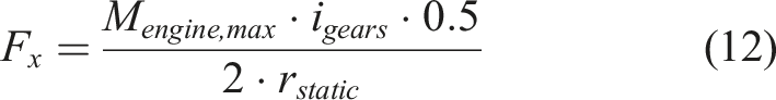

F_{x} = \frac{M_{engine,max} \cdot i_{gears} \cdot 0.5}{2 \cdot r_{static}}

(12)

A look at the measured speed of a load machine shows an evident overshoot (≈40 rpm) for the area of interest, which is independent of the initial speed. This behaviour has already been described in Hübner and Prokop (2025) in more detail. Taking into account the slip definition equation (7), the speed overshoot therefore has a significant influence depending on the vehicle velocity. As the controller compensates the speed deviation, the slip values also fall. If considering a real tire, this could be interpreted as a slipping tire, which triggers a brake intervention (traction control system). Nonetheless, the source of this phenomenon is only present on the test rig, and as slip values increase, damping also increases, masking the actual phenomenon to be investigated. Therefore, the results cannot be directly applied to the actual driving test. Future to-dos were defined and discussed in Hübner and Prokop (2025).

If a ramp (Δt = 2 s) is driven instead of the ‘jump’ (Δt = 0.02 s), there is only a slight speed overshoot (≈5 rpm) and the slip model results in correspondingly more plausible values, taking into account the already mentioned harmonics of some tire models, Figure 12. In general, the MF-Tyre model shows larger slips, which also result in higher speeds.

Tests in full simulative environment

The tests are repeated in the CarMaker Office simulation environment to verify the considerations outlined above. Additionally the numerical stability of the tire model solver is tested. For this purpose, the test runs are transferred from CarMaker Testbed and only the vehicle model is edited. The vehicle model is cut free for use on the test rig on the powertrain. To use the model in the simulation, a virtual powertrain must be implemented. The parameters from Table 1 were used for this purpose. As all other parameters of the real test specimen are unknown, the default values in CarMaker are assumed. In addition to the default computing time, the system was also overclocked.

Figure 10 shows the resulting slip curve of a tire for the torque ramp from Figure 12 for each of the three initial velocities. On the left are the diagrams with the standard calculation step size (Δt = 1 ms) and on the right the diagrams of the overclocked simulation (Δt = 0.2 ms). All diagrams show slip curves that decay due to gas pedal excitation and reach a stable system state. The slip decreases at lower velocities due to the relationship between the vehicle’s translational velocity and the tire’s rotational speed. It should be noted in particular that, in contrast to the test rig variant, the transient linear tire model is stable and does not produce a decaying signal even for the previously critical constant velocity of v = 5 km/h. The slowly increasing slip due to tire run-in behaviour can be observed in the test from standstill.

Figure 10.

Slip curves (full simulative environment) for the default step size (left charts) and a overclocked step size (right charts) for ramp manoeuvre, μ = 1.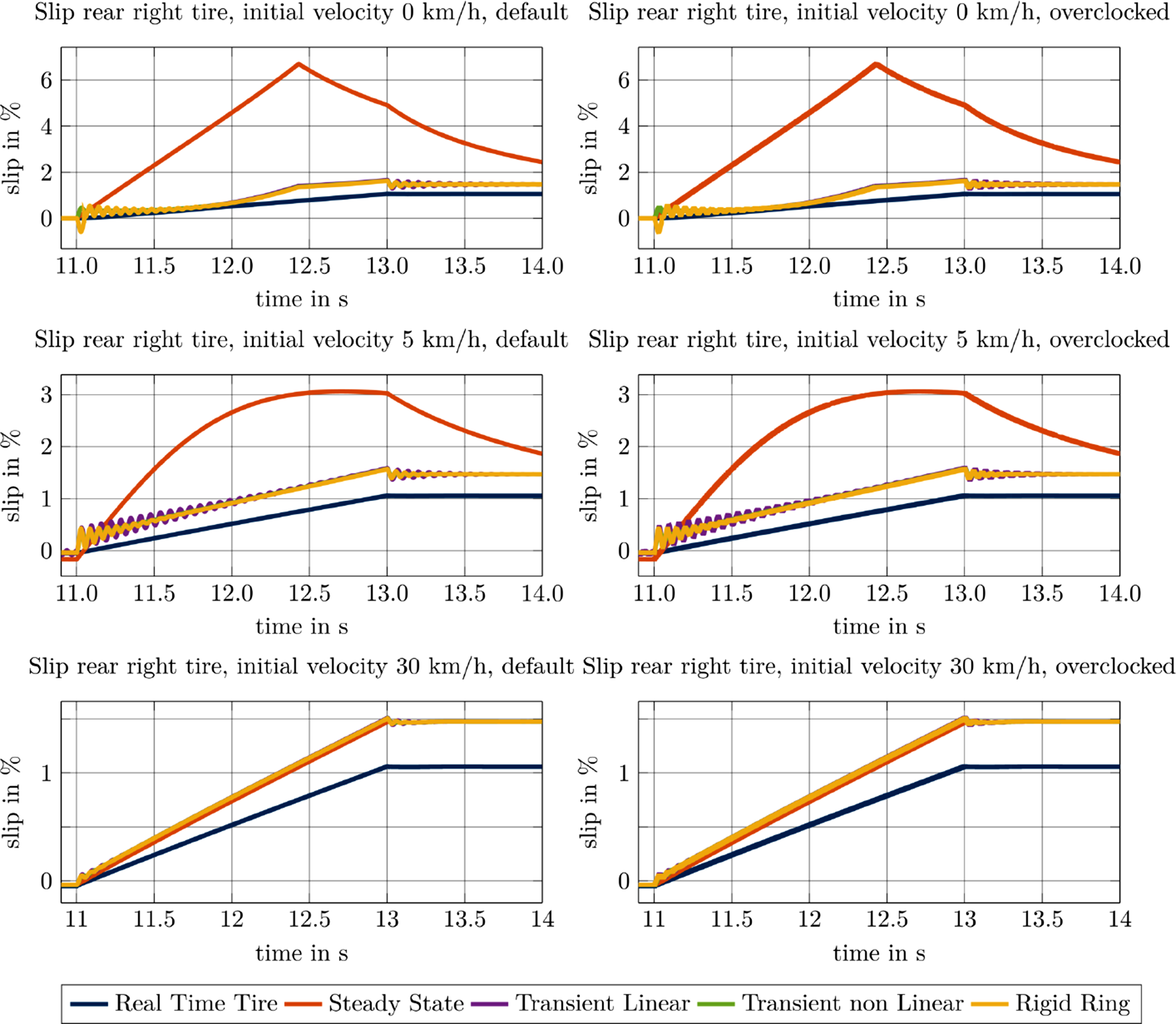

The initial peak at t = 11.2 s in Figure 12 does not occur in the simulation, which confirms the conclusion that this is a special test rig phenomenon. The diagrams of the standard step size and the overclocked system show no significant differences.

Figure 11 shows the resulting slip curve of a tire for the tip-in manoeuvre for each of the three initial velocities. In particular, the diagrams for v = 5 km/h and 30 km/h show decaying oscillations due to the jump excitation to a stable final value. Only the rigid ring and the transient non-linear tire model exhibit brief tire sliding during the manoeuvres from standstill, which then decays to a stable final value. The initial slip increase in Figure 9 at t = 11.2 s, which is not characterised by a pure damped oscillation, does not occur in the simulation. This also indicates that it is a test rig phenomenon. Apart from this, the absolute values of the slip due to the jump should also be scrutinised, especially given that the longitudinal force curves and the virtual engine torque indicate full traction, except for the two manoeuvres described.

Figure 11.

Slip curves (full simulative environment) for the default step size (left charts) and an overclocked step size (right charts) for tip-in manoeuvre, μ = 1.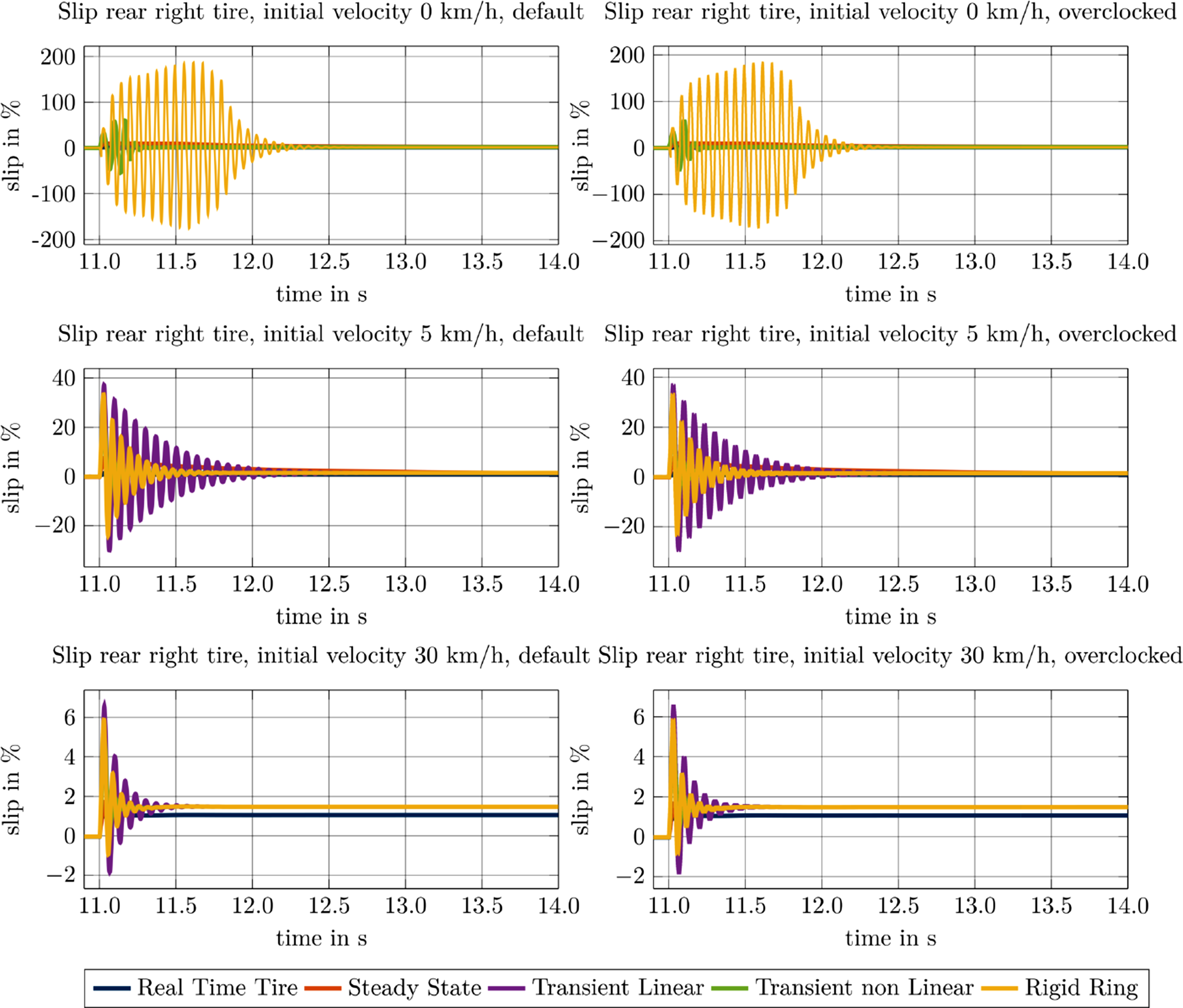

The MF-Tyre/MF-SWIFT model shows plausible results for ramps and manoeuvres from rolling motion. However, for jumps from low velocities or from a standstill, the data set used seems to reach its limits. The simulation results, in particular the stable signals, suggest that the models themselves can be used safely. For use on the test rig, a higher communication frequency and an overclocked simulation can be helpful.

Conclusion

To determine the influence of the tire model on the longitudinal vehicle shuffle in a coupled full vehicle simulation with a test rig of two highly dynamic load machines and an EDU, five variants were compared in this paper: the default IPG RealTime tire and the steady state, transient linear, transient non-linear and rigid ring dynamic models of the MF-SWIFT model, with combined slip model.

Concerning the questions formulated at the beginning, it has been shown that:

(1) The feasibility of the tests in HiL is heavily dependent on the selected settings of the tire model. In contrast to the pure software environment, this excludes some setting options, such as the pure consideration of longitudinal slip during a longitudinal acceleration manoeuvre. Depending on the solver used and the latency in communication, the demand values can implement vibrations on the HiL, which physically affect the EDU or influence the measurement results. The safety of the test specimen/test rig (limit set) must always be taken into account to ensure safe operation.

(2) The evaluation of the tests shows that the choice of tire model insignificantly influences the position of the frequency of the longitudinal vehicle shuffle. On the other hand, the complexity of the model, respectively, the consideration of higher, partly non-linear slip states, has a significant influence on the damping of the oscillation. With increasing slip values, the damping influence rises. This result is consistent with the findings in the literature and shows the validity of the physical mechanism in the cyberphysical system.

Depending on the manoeuvre to be driven, respectively, the vehicle characteristic to be analysed, the selection of the tire model is to be discussed, independent of the use in simulation or test rig. While simple tire model approaches may be sufficient for topics like traffic simulation, more complex models can be needed for vehicle physics and driving comfort. As seen in this investigation, the model complexity heavily influences the damping characteristics. The use of complex approaches results in the need for computing power and initial costs for procurement. Whether using commercial models like MF-Tyre, etc., or their own approaches has to be decided by the user themselves.

The investigation of both the simulation and HiL test runs shows that the used MF-SWIFT model reaches its limits when subjected to high transient load changes at low vehicle velocities or from a standstill.

Due to over- or undershoots in the speed signals of the load machines, the calculated slip values of the virtual wheel are influenced and reach unplausible dimensions for the manoeuvres shown. This behaviour is a special phenomenon for step functions and is caused by strongly different dead times of the paired machines and the controller used. The transferability of road-matching approaches of the current system has to be assessed critically.

The oscillations that occur in the transient linear and rigid ring model in HiL need to be investigated in greater depth. Due to the lack of access to the internal calculations, the models themselves must be regarded as a black box.

Nonetheless, the phase response due to the latency between the vehicle simulation (XPack4) and the frequency converter (via SPARC) must be analysed first for the open loop and then for the closed loop connection. Based on this, further adjustments to the current signal transmission (transmission frequency: 1 kHz) must be made to reduce the latency, for example, by overclocking. However, this requires support from both the test rig manufacturer and the manufacturer of the vehicle simulation. This approach can lead to significantly more stable speed signals and thus ultimately make it easier to analyse the vehicle shuffle, which will be part of further investigations.

Footnotes

Acknowledgements

This report was written in German and translated into English. KI (DeepL) was used for this purpose.

ORCID iD

Carl Hübner

Funding

The authors received no financial support for the research, authorship, and/or publication of this article.

Declaration of Conflicting Interests

The authors declared no potential conflicts of interest with respect to the research, authorship, and/or publication of this article.

Appendix

Table 5.

Mean backlash B_mean and acceleration a_{min, maxmean} values (with standard deviation) of the longitudinal vehicle shuffle depending on the tire model.

Value	RealTime	SteadyState	TransientLinear^a	TransientNonLinear	RigidRing^a
in m/s²	μ = 1
B _mean	0.20	0.21	–	0.48	-
σ _B	0.04	0.05	–	0.06	-
a _max	2.39	2.45	–	2.72	-
σ _amax	0.04	0.03	–	0.06	-
a _min	2.18	2.24	–	2.24	-
σ _amin	0.03	0.03	–	0.03	-
in m/s²	μ = 0.5
B _mean	0.23	0.21	–	0.42	–
σ _B	0.06	0.03	–	0.07	–
a _max	2.41	2.45	–	2.65	–
σ _amax	0.05	0.03	–	0.09	–
a _min	2.18	2.24	–	2.23	–
σ _amin	0.03	0.03	–	0.03	–

^aA low-pass filter is applied to the data in order to dampen superimposed oscillations.

References

Andert

Xia

Klein

, et al. (2018) Road-to-rig-to-desktop: virtual development using real-time engine modelling and powertrain co-simulation. International Journal of Engine Research 20(7): 686–695.

Brayanov

Stoynova

(2019) Review of hardware-in-the-loop - a hundred years progress in the pseudo-real testing. E+E 54: 70–84.

dos Santos

Guimaraes

Da Silva

, et al. (2018) A method to calculate hardware in the loop applications representativeness. SAE Technical Paper 36: 0171.

Dresig

Holzweißig

(2016) Maschinendynamik. 12th ed. Wiesbaden: Springer Vieweg.

Düser

(2010) X-in-the-Loop – Ein Durchgängiges Validierungsframework Für Die Fahrzeugentwicklung Am Beispiel Von Antriebsstrangfunktionen Und Fahrerassistenzsystemen. Karlsruhe: Karlsruher Insitut für Technologie.

Fan

(1994) Theoretische und Experimentelle Untersuchungen zu Längsschwingungen von Pkw (Ruckeln). In: Berichte Aus Der Fahrzeugtechnik. Aachen: Shaker.

Figel

Schultalbers

Svaricek

(2019) Review and experimental evaluation of models for drivability simulation with focus on tire modeling. Forschung im Ingenieurwesen 83(2): 105–118.

Hübner

Prokop

(2025) A preview for vehicle driveability characterization on subsystem level powertrain. Advances in Mechanical Engineering 17(11). doi: 10.1177/16878132251383227.

Hülsmann

(2007) Methodenentwicklung Zur Virtuellen Auslegung Von Lastwechselphänomenen in Pkw Dissertation. München: Technische Universität München.

10.

Hüsemann

(2013) Fahrdynamik: Kraftübertragung zwischen Reifen und Fahrbahn. In: Heißing

Ersoy

Gies

(eds) Fahrwerkhandbuch. Wiesbaden: Springer Fachmedien Wiesbaden, 56–70.

11.

IPG Automotive GmbH (2023a) Carmaker Reference Manual, Vol. 1.Version 12.0.

12.

IPG Automotive GmbH (2023b) Carmaker user’s guide: Version 12.0.1.

13.

Lukac

Brumercik

Krzywonos

(2016) Driveability simulation of vehicle with variant tire properties. Communications - Scientific letters of the University of Zilina 18(2): 34–37.

14.

Lunze

(2020) Regelungstechnik 2: Mehrgrößensysteme, Digitale Regelung. 10 ed. Wiesbaden: Springer Vieweg.

15.

Pacejka

(2012) Tire and Vehicle Dynamics. 3th ed. Amsterdam: Elsevier.

16.

Pillas

(2017) Modellbasierte optimierung dynamischer fahrmanöver mittels Prüfständen. Darmstadt: Technische Universität Darmstadt.

17.

Schmidt

Prokop

(2023) Experimental analysis of powertrain test bed dynamometers for Black box-based digital twin generation. In: Transportation Electrification Conference & Expo (ITEC) 2023, 1–6. IEEE.

18.

Schmidt

Büttner

Prokop

(2023) Methods for virtual validation of automotive powertrain systems in terms of vehicle drivability - a systematic literature review. IEEE Access 11: 27043–27065.

19.

Schramm

Hiller

Bardini

(2013) Modellbildung Und Simulation Der Dynamik Von Kraftfahrzeugen. Berlin, Heidelberg: Springer Berlin Heidelberg.

20.

Siemens Digital Industries (2022) Simcenter tire: mf-Tyre/mf-swift: user manual version 2212.

21.

Sorniotti

(2008) Driveline modeling, experimental validation and evaluation of the influence of the different parameters on the overall system dynamics. SAE Technical Paper: 1.

22.

Verein Deutscher Ingenieure (2017) Einwirkung Mechanischer Schwingungen Auf Den Menschen: Ganzkörperschwingungen. VDI-Richtlinien: VDI 2057 Blatt 1. Düsseldorf.

23.

Zegelaar

PWA

(1998) The Dynamic Response of Tyres to Brake Torque Variations and Road Unevennesses. Dissertation: Delft University of Technology.

The impact of tire simulation approaches on the longitudinal vehicle shuffle in a cyberphysical environment

Abstract

Keywords

Introduction

Tire models

RealTime Tire

MF-Tyre

MF-SWIFT

HiL application for driveability investigation

HiL setup

Tire model settings

Manoeuvre definition

Analysis of measurements

Solver analysing

Pedal jump

Plausibility check

Tests in full simulative environment

Conclusion

Footnotes

Acknowledgements

ORCID iD

Funding

Declaration of Conflicting Interests

Appendix

References