
Abstract
In this study, we introduce a machine learning-based method to predict the modeling parameters of superelastic shape memory alloys (SMAs). Our goal is to simultaneously determine and fine-tune all internal and material-related parameters, including thermodynamic ones, for a specific constitutive model using only cyclic tensile tests. We employ feedforward neural networks (FNNs) for their versatile structure. First, we sample the searched parameters within a predefined parameter space using the Latin hypercube sampling method. Then, using the constitutive model with the sampled parameters and representative strain loading, we generate the corresponding stress responses and finally train the FNN. To address the ill-posed nature of this inverse parameter identification problem and ensure a unique parameter set, during training, we use a dual network architecture with an additional FNN-based surrogate of the constitutive model. We also utilize transfer learning to accelerate the training process through knowledge transfer and handle multiple load cases simultaneously, ensuring consistent parameter identification across different scenarios. We validate the method by comparing the numerical results with the experimental data and demonstrate the importance of accurately identified parameter sets by numerical investigations on a SMA-retrofitted frame structure.
Keywords
1. Introduction
Shape memory alloys (SMAs) constitute a class of two-phase polycrystalline metals that respond superelastically (pseudoelastically) during austenitic steady-state. Under dynamic loading, energy dissipation occurs due to repeated phase transformations between the austenite and martensite states, as described in detail by Altay (2021). In addition to their exceptional energy dissipation capabilities, SMAs possess distinct attributes, such as high deformation recovery, resistance to corrosion, and low fatigue. Compared to the shape memory effect, superelastic behavior is solely driven by mechanical loads without the need for additional temperature input. Consequently, superelastic SMAs have attracted substantial interest in the field of civil engineering, particularly in structural vibration control. For instance, Han et al. (2005) developed an SMA wire-based damper, which simultaneously reduces vibrations under tension, compression, and torsion loading. Furthermore, AlSaleh et al. (2012) studied the vibration behavior of SMA wires in retrofitting applications. More recently, Nekouei et al. (2020) conducted numerical studies on the dynamic behavior of hybrid laminated composite cylindrical shells reinforced with SMA fibers. A comprehensive overview of applications related to seismic protection can be found in the book of Fang and Wang (2020). The recent review of Tabrizikahou et al. (2022) includes examples of further applications.
The design of control devices incorporating SMAs requires accurate constitutive models. A notable uniaxial model was introduced by Auricchio et al. (2008). For numerical efficiency, macroscopic models are generally favored. Common forms of SMAs, such as wires, cables, or rods, are preferred in control devices due to their ability to facilitate efficient heat transfer. While these forms are prevalent, other SMA configurations exist, with examples provided by Fang (2022). For a comprehensive review of various SMA modeling techniques, the reader is referred to the work of Cisse et al. (2016) and the references therein.
Particularly during dynamic loading, SMAs may exhibit extensive thermodynamic effects. Their accurate representation in constitutive models poses a significant challenge and necessitates the precise identification of model parameters. Beyond conventional cyclic tensile tests, additional experiments, such as those for thermodynamic parameters, might be necessary (Elwaleed (2018)). Furthermore, for internal model parameters that lack a direct correlation with any physical quantity, a subsequent tuning procedure is usually required. Gradient-based optimization algorithms are often employed to solve these problems, such as in Hartloper et al. (2021). However, for high-dimensional parameter spaces and ill-posed problems, gradient-based algorithms can become computational inefficient due to ill-conditioned objective functions. To overcome these challenges, machine learning techniques, such as artificial neural networks (ANNs), harbor efficient solutions. In this context, ANNs are advantageous as they are robust to noisy data, can handle non-linear problems, offer end-to-end learning, and are easy to implement. Although weights and biases of ANNs must be optimized, the optimization problem is often easier to solve as in this case the gradients are not directly computed with respect to the desired parameters themselves. Here, the ANN learns the mapping between the desired functions and the corresponding parameters over a whole parameter space. Therefore, the gradients of the objective function are computed with respect to the weights and biases of the network. To train ANNs effectively, the data set must be of high quality with a sufficient quantity of respresentative data pairs. In addition, an appropriate set of hyperparameters has to be selected and is crucial to provide accurate predictions.
Similar techniques have been adopted for the forward modeling of SMAs. For instance, Ozbulut and Hurlebaus (2010) employed an adaptive neuro-fuzzy inference system (ANFIS) for seismic applications. Another approach, recently proposed by Shao and Andrawes (2022), utilized feedforward neural networks (FNNs), a type of ANNs, to predict the seismic drift of a reinforced concrete column retrofitted with superelastic SMA wires. Additional examples of forward modeling in other SMA applications, such as actuators, can be found in the review by Hmede et al. (2022).
For the identification of SMA parameters, optimization-based methods have been proposed, such as by Meraghni et al. (2014). Although these methods have proven to be powerful, the advent of ANNs has introduced techniques that are efficient and easier to implement. A pioneering example of this was presented by Helm (2004), who employed FNNs with stress as an input for SMAs under quasi-static loading. Furthermore, for SMA actuators, Henrickson et al. (2013) employed an FNN architecture, which required strain and temperature responses as input.
In our prior study (Lenzen and Altay (2022)), we introduced a deep FNN architecture that required only stress responses as input to identify SMA parameters under dynamic loading. We intentionally chose FNNs in our method primarily due to their adaptability across different scenarios and their simplicity in terms of hyperparameter tuning and model fitting. Compared to other network architectures, FNNs offer a less complex setup, which significantly eases the process of training. Additionally, FNNs are known for their computational efficiency, making them more practical and faster to deploy than their more complex counterparts. In this case, we implemented the methodology for a constitutive model proposed by Zhu and Zhang (2007), identifying its three thermodynamic parameters and one internal parameter. Our subsequent studies (Lenzen et al. (2023)) have revealed that as the number of parameters increases, the precision can be compromised due to the ill-posed nature of the identification process. One potential solution could be to constrain the parameter space. However, this approach would require expert knowledge about the SMA specimens, which might not always be available.
In the present study, we address this challenge by pairing the initial FNN (inverse model) with a second FNN (forward model) that has been pretrained to serve as a surrogate for the constitutive model. Supervised training of these coupled FNNs requires only stress responses. Originally adopted in other fields (Long et al. (2019); Kumar et al. (2020)), this dual network architecture enables the inverse model to discern unique solutions to identify model parameters based on stress responses of the SMAs. We train for each relevant load case separately and employ transfer learning (Bozinovski (2020)) to accommodate multiple load cases in the identification process. As a result, we simultaneously ensure consistent parameter identification across different load cases. The key contributions of this study are: • Simultaneous identification of a vast array of parameters through tensile testing, eliminating the need for additional thermodynamic experiments and calibration. • Resolution of the ill-posed nature of the parameter identification problem through the implementation of a dual network architecture, which is critical for robust parameter estimation in SMA models. • By employing transfer learning, our approach handles multiple load cases simultaneously, ensuring consistent parameter identification across different scenarios.
We would like to emphasize that the proposed method does not aim to model the responses directly; instead, it provides parameters for existing material models. Our work addresses the critical gap of parameter identification of SMA models, an area that continues to be an open research issue. Existing methods, such as gradient-based approaches, often struggle due to the ill-posed nature of this problem. Accurate parameter identification is particularly essential for the successful implementation of complex material models, such as in applications involving dampers in civil engineering structures.
The structure of this paper is organized as follows. The section titled Parameter Identification Methodology introduces the identification method and details its implementation within the macroscopic models proposed by Auricchio et al. (2008) and Zhu and Zhang (2007), models that require numerous parameters. In the Results and Discussion section, we explore various influences on the training performance and accuracy of our method, including network architecture, sample size, and transfer learning. This is followed by the presentation of experimental results, serving to validate our findings. We also demonstrate the importance of accurately identified parameter sets by numerical investigations on a shear frame structure retrofitted with dampers incorporating superelastic SMA wires. We conclude with the Conclusions section, summarizing the key insights from our study and suggesting directions for future research.
2. Parameter Identification Methodology
2.1. Rate-dependent superelastic material response
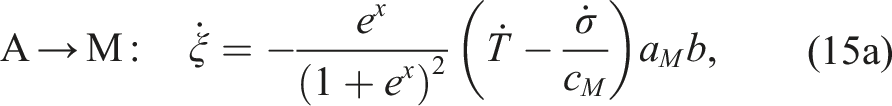
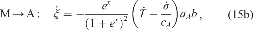
SMAs are distinguished by their two crystalline phase states; austenite (A) and martensite (M). When the material temperature exceeds the austenite finish temperature A f , SMAs exhibit superelastic behavior with austenite as the parent phase. Under high mechanical stresses, a forward phase transformation (A → M) occurs, causing SMA crystals to reorient their atomic lattice from a body-centered structure to a monoclinic structure, which is more stable at higher stresses. During unloading, a reverse phase transformation (M → A) follows, restoring the material to its initial shape with no residual deformation. Both forward and reverse phase transformations lead to pseudoelastic deformations, which are manifested as stress plateaus in the stress–strain response.
The forward transformation is exothermic and generates internal heat, which is dissipated to the environment through heat convection and conduction. On the contrary, the reverse transformation is accompanied by endothermic processes, causing a reduction in the material temperature during austenite formation. For high-rate cyclic loading, delays in heat transfer to the surrounding cause an increase in material temperature and simultaneously suppress the forward transformation as described by the Clausius–Clapeyron relation and evidenced by studies, such as those conducted by Kaup et al. (2021a).
During high strain rate, SMAs start forward transformation at higher stress levels. In this case, the martensite formation is suppressed by the increase in the material temperature. During the unloading, austenite formation is favored so that reverse transformation is initiated at higher stress levels. As a result, the hysteretic surface shows significant changes, indicating a direct effect on the energy dissipation. Predicting this dynamic response requires complex models with multiple parameters, which need to be identified and tuned accurately.
2.2. Constitutive modeling
To demonstrate the implementation of parameter identification, we use two different uniaxial thermomechanical models. The first model was originally developed by Auricchio et al. (2008) and was later extended by Kaup et al. (2019). The second model origins from Zhu and Zhang (2007) and was updated in Kaup et al. (2021b).
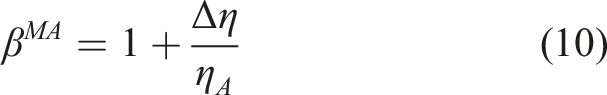
2.2.1. Auricchio model
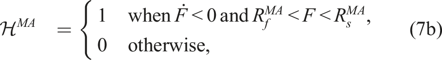
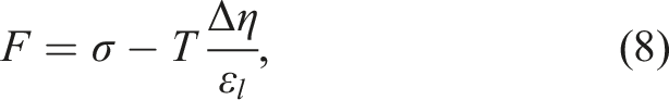
The model computes from strain ɛ and strain rate
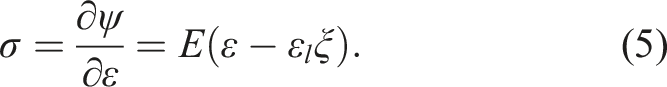
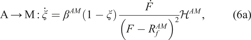
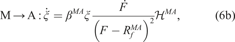
where F is the driving force;
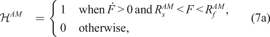
where
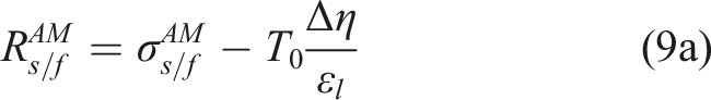
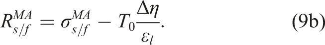
Here,
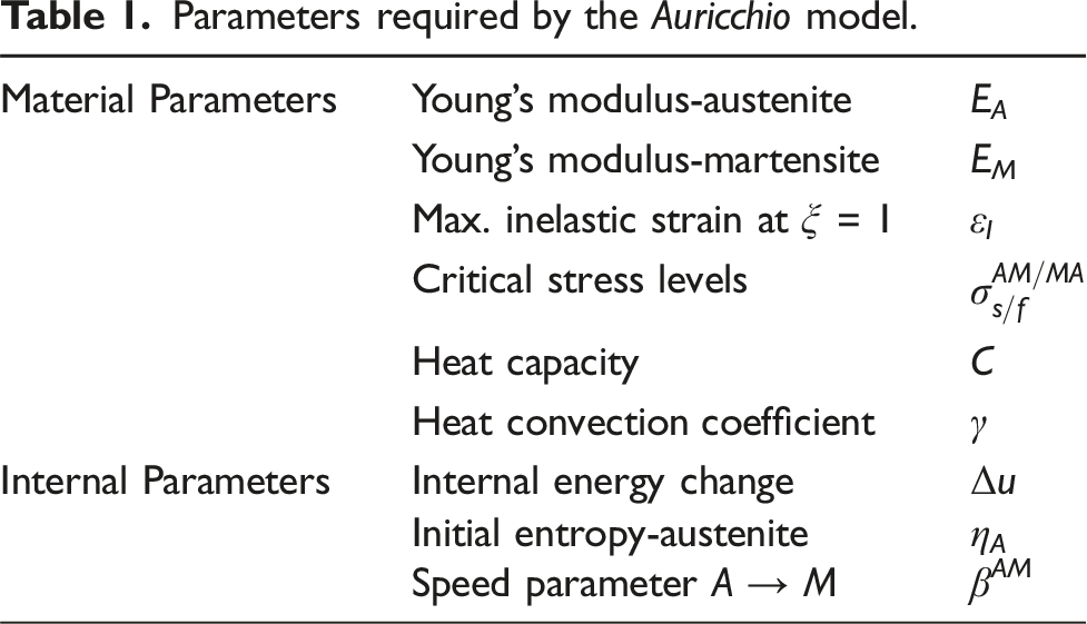
Parameters required by the Auricchio model.
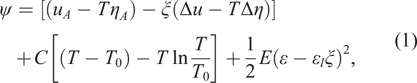
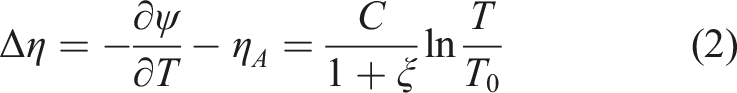
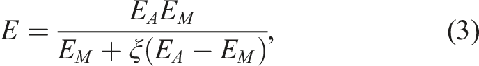
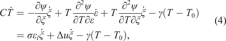
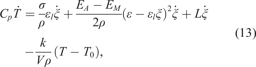
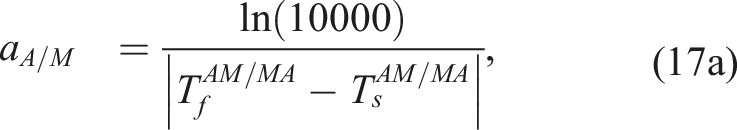
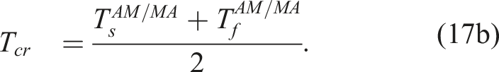
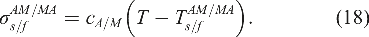
2.2.2. Zhu and Zhang model
The model is strain- and strain rate-driven and computes the resulting temperature T, martensite volume fraction ξ and stress σ responses based on the following free energy formulation: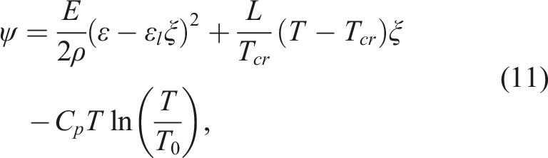


where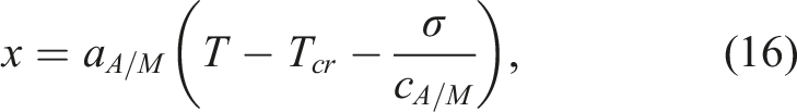
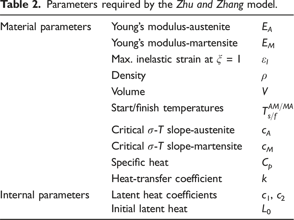
Parameters required by the Zhu and Zhang model.
2.3. Parameter identification
The constitutive model can be expressed as Steps involved in preparation of the inverse model. (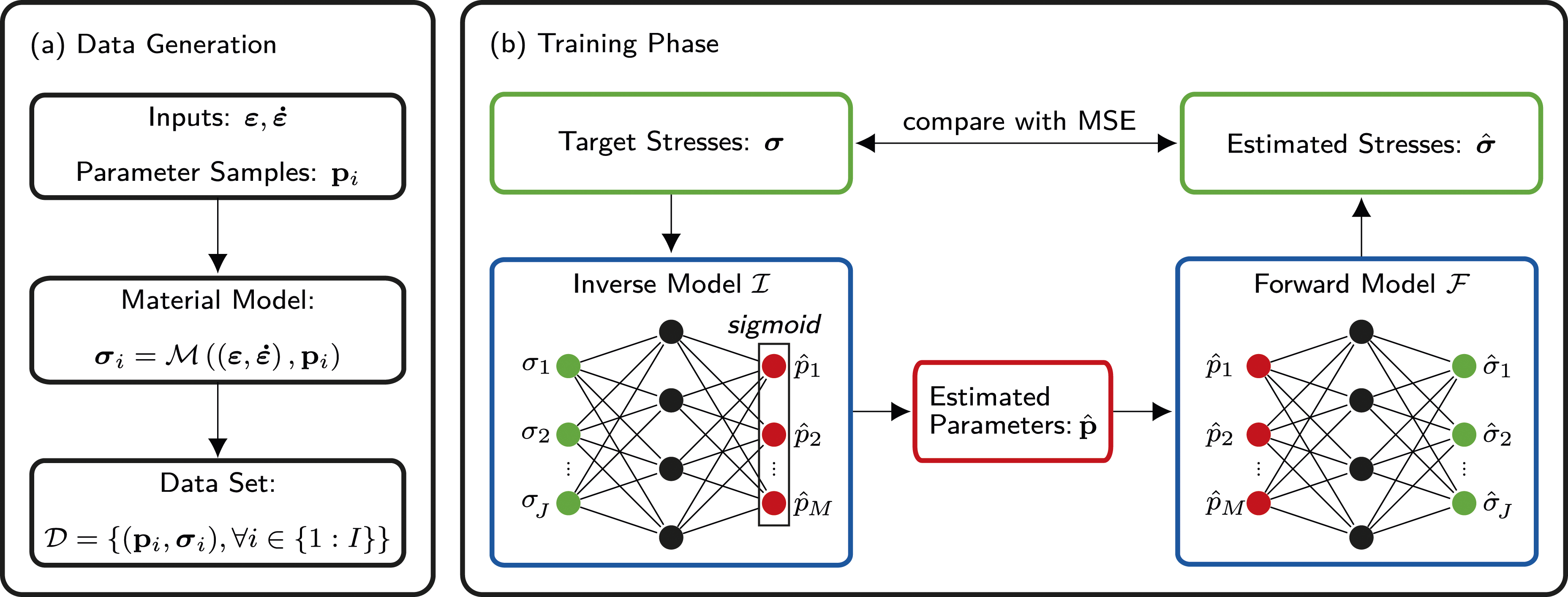
The data set
To cover all characteristics of the investigated SMA wires, such as strain rate effects, a variety of representative load cases has to be considered. To optimize the choice of load cases, active learning strategies can be applied, as proposed by Milicevic and Altay (2023). These strategies can be quite useful to reduce the experimental and computational costs in cases where a large variety of loads is required or the parameter space spans a wide area. However, in this study, as the training data is not generated experimentally and can be efficiently obtained by the material model, active learning strategies are not required. Each set of sampled parameters
Due to the ill-posed nature of the problem, training an FNN to directly map the stress response to parameters can yield poor results, as the FNN might inadvertently penalize valid parameter combinations. To avoid this, a dual network architecture as illustrated in Figure 1(b) is employed, where the training phase is divided into two steps. First, a forward model 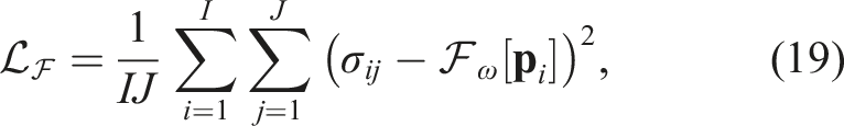
Subsequently, we introduce the inverse model 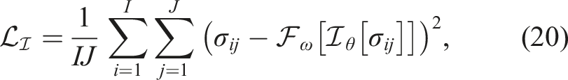
It is important to note that the forward model is limited to producing the stress responses corresponding to the strain and strain rate time histories utilized for the data generation. Therefore, to accommodate multiple load cases, distinct forward and inverse models are trained for each specific case. To accelerate the training process, transfer learning (Bozinovski (2020)) is employed. Once the initial forward and inverse models are trained, this technique is applied to train the models for subsequent load cases. More importantly, this approach ensures consistent parameter identification across different loading scenarios, as the weights and biases originate from a consistent initial region within the predefined parameter space.
Several additional key features are crucial during training. We incorporate the batch normalization algorithm (Ioffe and Szegedy (2015)) along with the Adam optimizer (Kingma and Ba (2014)). In the hidden layers, the ReLU activation function is paired with the He initializer, in line with the suggestions by He et al. (2015). The sigmoid activation function is specifically employed in the output layer of the inverse model to ensure that its outputs lie between 0 and 1 and initialized by the Glorot initializer (Glorot and Bengio (2010)). This constraint is vital to avoid exceeding the boundaries of the parameter space. Furthermore, a linear activation function is implemented in the final layer of the forward model.
3. Results and Discussion
3.1. Auricchio model
We aim to identify the parameters of the constitutive model for a Nitinol wire sample with alloy composition Ni-55.8% and Ti-43.55%, manufactured by SAES Getters S.p.A. The known parameters are as follows: • Young’s modulus-austenite: E
A
= 32,350 MPa • Young’s modulus-martensite: E
M
= 18,550 MPa • Max. inelastic strain at ξ = 1: ɛ
l
= 3.3%
As outlined in the Methodology section, nine parameters need to be identified using an appropriate FNN (inverse model). These include the four critical stress levels
3.1.1. Data generation


Sample space of the searched parameters of the Auricchio model.
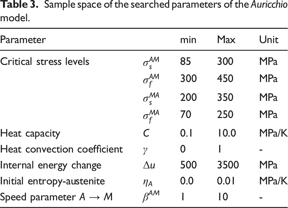
However, as the FNNs will be trained to reconstruct the target stresses, our parameter identification method can deal with unreasonably chosen samplings. More precisely, the FNNs will be able to identify a parameter set that can represent the desired stress response whether this set respects these rules or not. The only requirement is that the desired stress response is covered by the parameter space during training. In fact, our parameter identification method provides the user flexibility in defining the parameter space, such that a suitable parameter set can be found without requiring expert knowledge about the material model. In general, the parameter space could also be chosen such that the rules are respected. For this purpose, the user must inspect the experiments and also have knowledge of the material model.
Utilizing the constitutive model, we compute the stress responses for these combinations of sampled parameters, assuming an ambient temperature of T0 = 296 K (approximately 23°C). We employ strain and strain rate time histories with J = 200 time instants and a time step size of Δt = 0.001 s. Given that these computed 200 stress responses serve as inputs for the inverse model and outputs for the forward model, the value of J dictates the number of neurons in the respective layers. In Training subsection, we provide further information on the choice of the remaining network architectures.
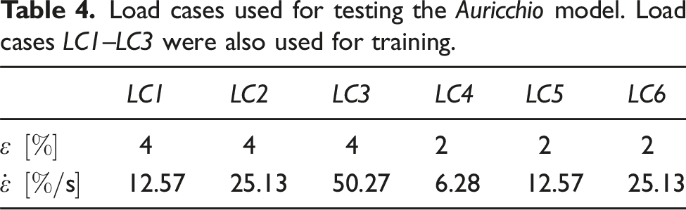
Load cases used for testing the Auricchio model. Load cases LC1–LC3 were also used for training.
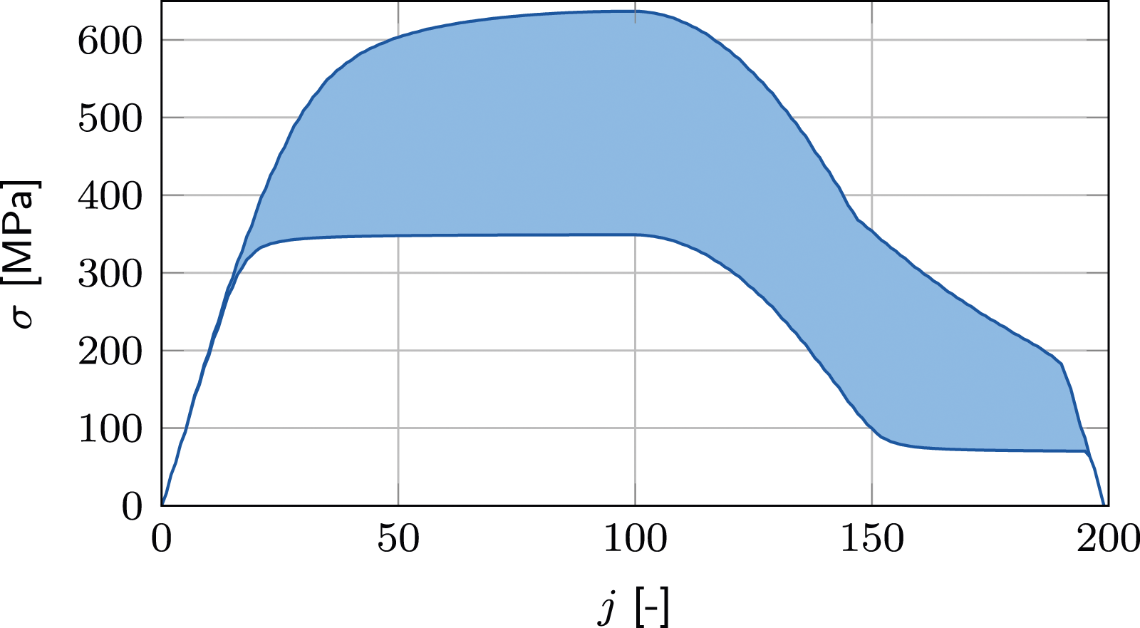
Stress response range covered by 10 of sampled parameter combinations for LC1. Each response time history has J = 200 time instants.
Of the total generated data, 90% is used for training purposes, reserving the remaining 10% for validation. After training, we test the models using
To enhance robustness and provide a buffer against potential measurement inaccuracies, we incorporate a Gaussian noise with a zero mean and a variance of 1 ⋅ 10−3 to all the computed stress responses.
3.1.2. Training
The hyperparameters for both the inverse and the forward models are fine-tuned through testing various configurations. For all studies, the mini-batch gradient descent method is employed for training with a batch size of n b = 1000. As the training data set is generated synthetically by the constitutive model and enriched with Gaussian noise, the data set does not contain any outliers such that the MSE is chosen for the training process.
3.1.2.1. Effects of network architecture
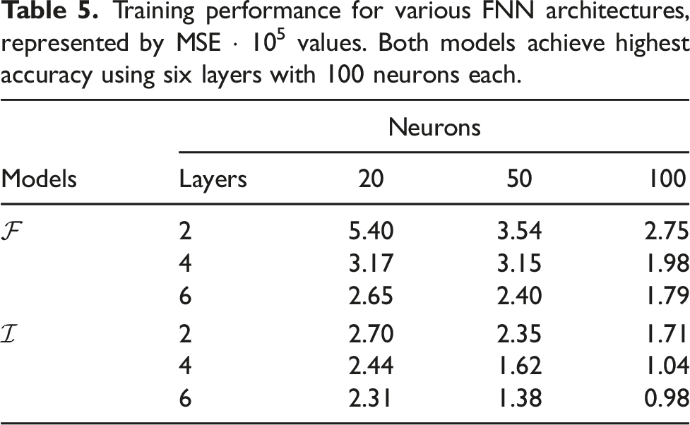
Training performance for various FNN architectures, represented by MSE · 105 values. Both models achieve highest accuracy using six layers with 100 neurons each.
3.1.2.2. Effects of learning rate
Using the optimal FNN architecture determined above, we assess the influence of different learning rates. Initial weights and biases remain consistent across all configurations. For this evaluation, we sample I = 40 ⋅ 103 parameter combinations and utilize n e = 2000 epochs with load case LC1. The MSE outcomes for both forward and inverse models are studied with the learning rates η = 0.1 ⋅ 10−3 to η = 1 ⋅ 10−3. The most effective learning rate is identified as η = 1 ⋅ 10−3 with a corresponding MSE value of 1.79 ⋅ 10−5 for the forward model and 0.98 ⋅ 10−5 for the inverse model.
3.1.2.3. Effects of number of sampled parameter combinations
We evaluate the MSE values of both models across various numbers of sampled parameter combinations, ranging from I = 10 to I = 100 ⋅ 103. This is depicted in Figure 3. The network architecture and learning rate selections are based on previous studies. For this analysis, we use n
e
= 2000 epochs with the load case LC1. The data reveals that by the time I reaches 40 ⋅ 103, the MSE values for both models converge to a notably low value. MSE values corresponding to varying numbers of training samples. Both models converge to a low MSE value at I = 40 ⋅ 103.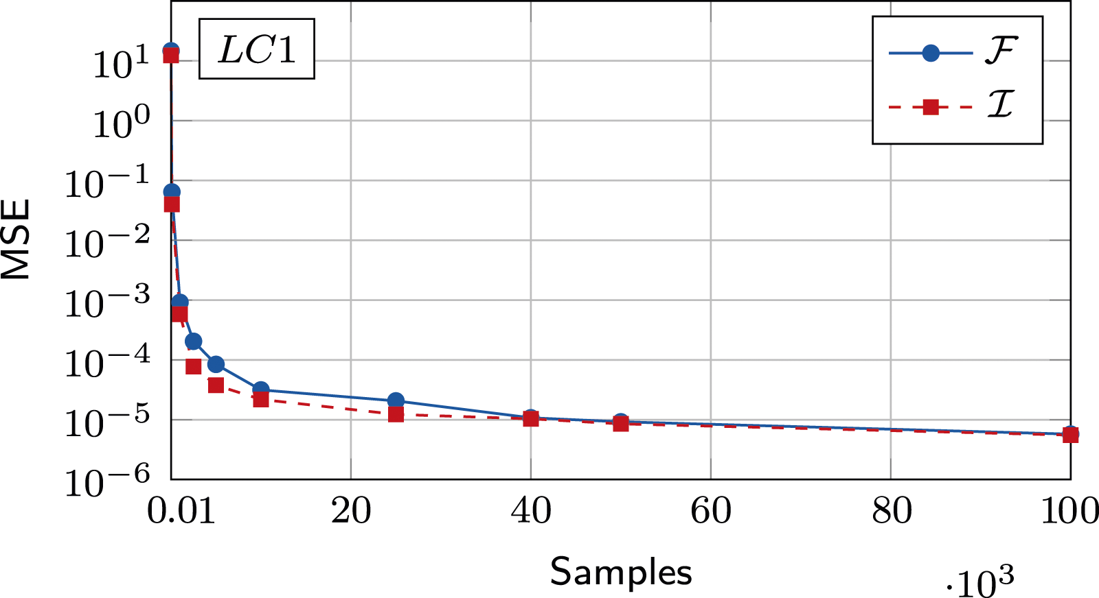
3.1.2.4. Effects of number of epochs
Figure 4 illustrates the impact of the number of epochs on the training loss for both the forward and the inverse models. The best architecture and learning rate, determined from previous studies, are used along with the load case LC1. For this analysis, I = 40 ⋅ 103 sampled parameter combinations are employed. Observing the results, it becomes evident that both models achieve convergence by n
e
= 2000 epochs. Effect of number of epochs on the training of the forward 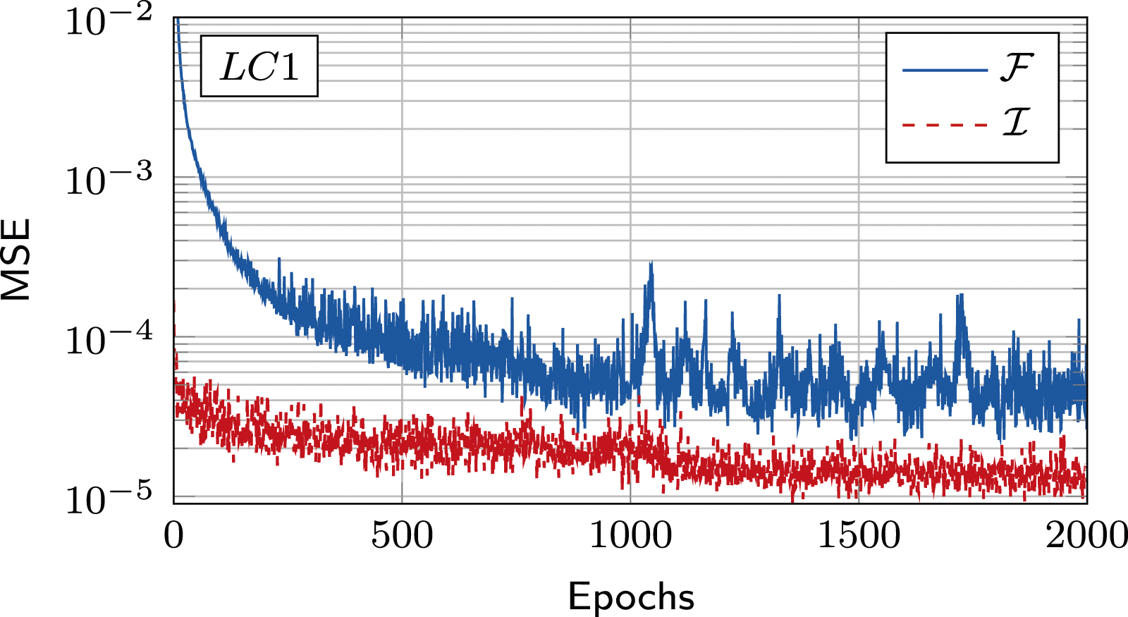
3.1.2.5. Effects of transfer learning
Training the models from scratch without shared weights and biases might result in parameter sets with notable disparities across different load cases. To derive a consistent parameter set across all load cases, we employ transfer learning. Additionally, transfer learning is also pursued to reduce the overall training effort.
For training, we select the optimal architecture comprising six layers with 100 neurons each. The learning rate is set at η = 1.0 ⋅ 10−3, and n e = 2000 epochs are used. Initially, the forward model is trained using load case LC1 for I = 40 ⋅ 103 parameter combinations. Subsequently, the weights and biases of this forward model are retained and employed for the training of the inverse model. This training methodology is then extended to load cases LC2 and LC3, leveraging the weights and biases from the LC1-trained models without reinitialization. Remarkably, this approach reduces the necessary epochs for LC2 and LC3 to a mere n e = 20, representing only 1.0% of the training effort compared to LC1.
Figure 5 proves the precision of the models for LC1 by juxtaposing the target stresses (obtained via the constitutive model) with the estimated values. In the first scenario, denoted as Comparison of stress estimation accuracy between the forward model 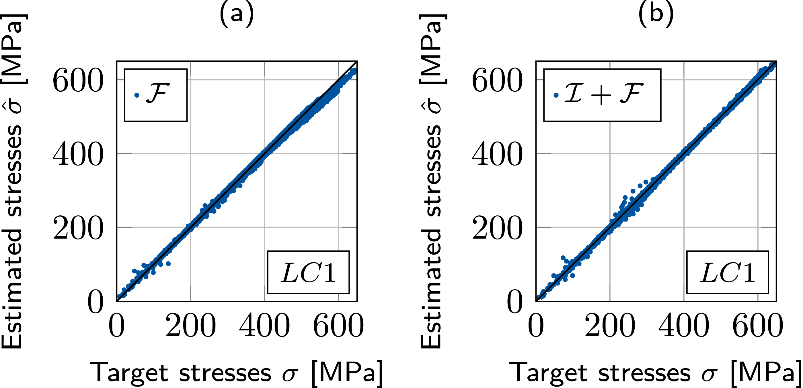
Figure 6 compares the target stresses, determined by the constitutive model, with the estimated stresses for the load case LC3. In the first case, Comparison of transfer learning effects. Models 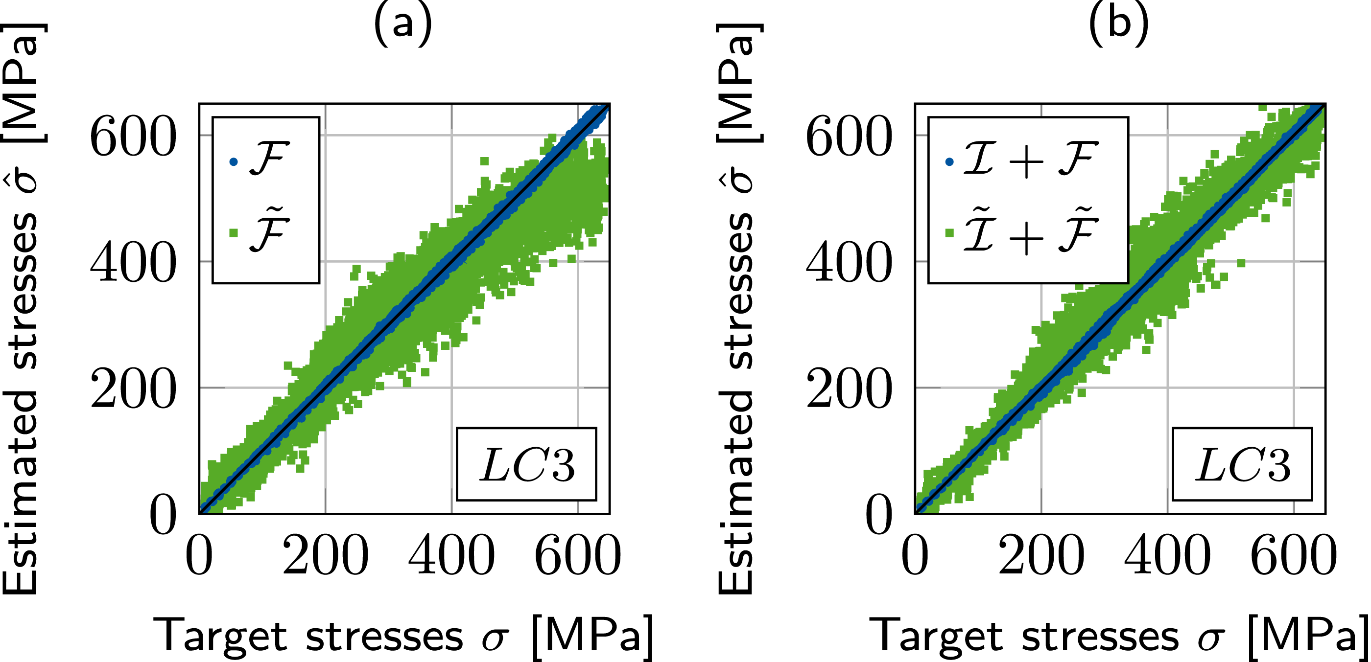
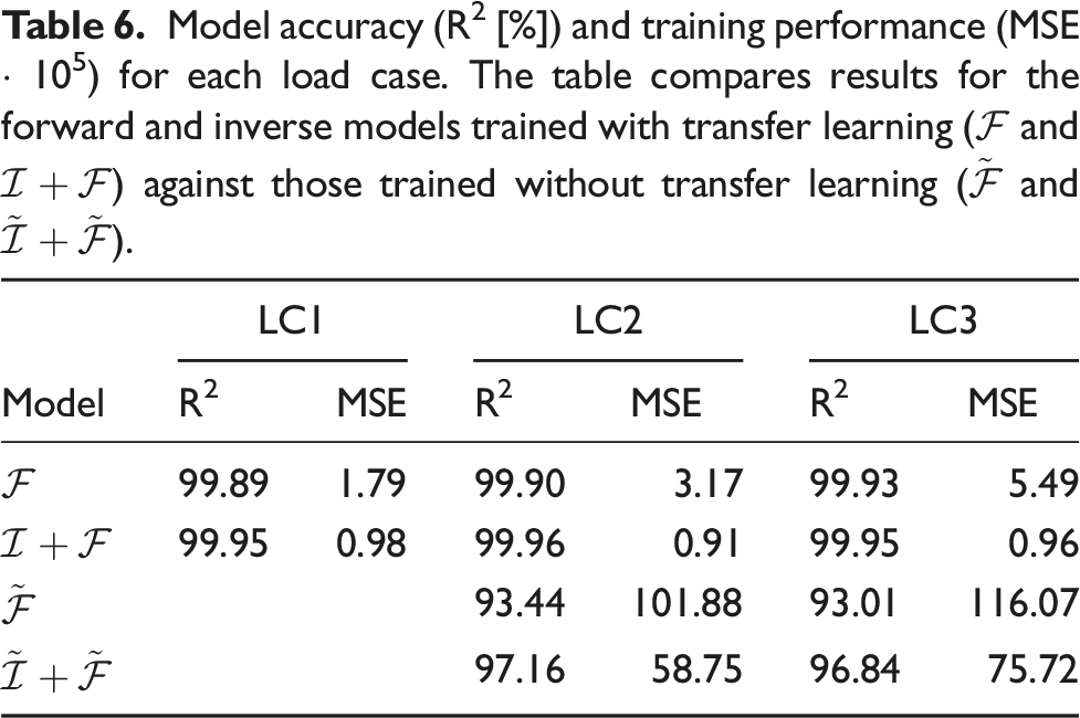
Model accuracy (R2 [%]) and training performance (MSE ⋅ 105) for each load case. The table compares results for the forward and inverse models trained with transfer learning (
3.1.3. Experimental validation
To validate the proposed methodology, we conducted stress–strain experiments and compared the outcomes with our estimations. The test setup, as illustrated in Figure 7, comprised a shaking table that can generate intricate uniaxial motion signals relative to a fixed test rig. An SMA wire specimen, with dimensions l = 150 mm in length and D = 0.2 mm in diameter, was examined. We mounted a load cell on the test rig to capture the stress response. To ensure that the load is applied centrally to the load cell and to prevent any buckling, a pulley system was utilized to redirect the wires. Weights were used to apply a pre-stress of σ0 = 134.9 MPa, facilitating the desired phase transformation at a strain level that matched the limits of the test setup. Additionally, the shaking table motion was continuously monitored using a laser sensor. Test setup used for the validation study: shaking table (a), test rig (b), SMA wire specimen (c), load cell (d), pulley (e), weights (f), motion direction (g), and laser sensor (h).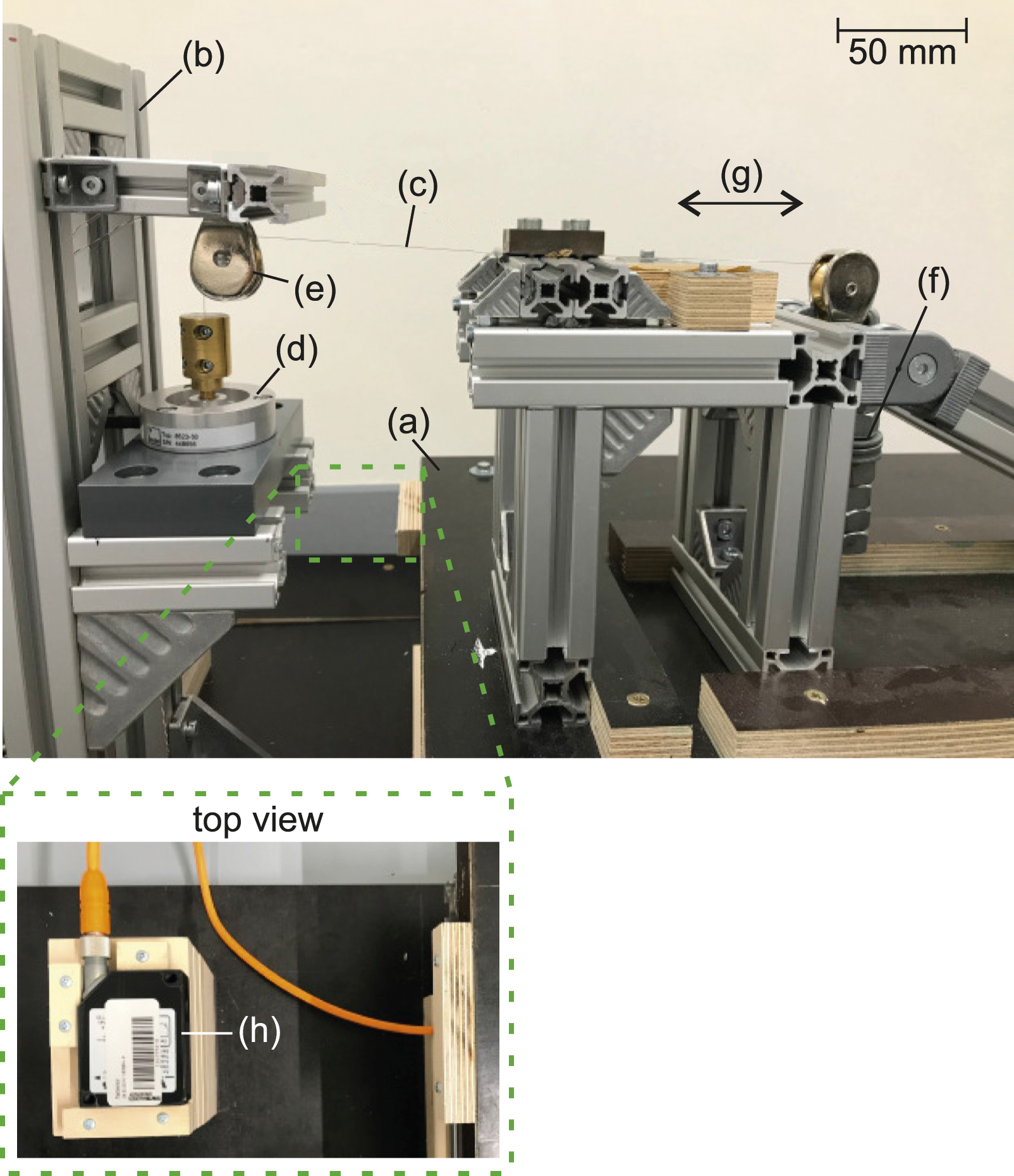
Throughout the experiments, the ambient temperature was maintained at approximately T0 = 296 K (approximately 23°C), which is consistent with the conditions assumed during data generation. For the identification of the parameters, we first executed experiments for the same load cases, namely LC1–LC3, that were employed during the model training. Moreover, the number of time instants and the time step sizes selected for the experiments corresponded to those used in the training of the models.
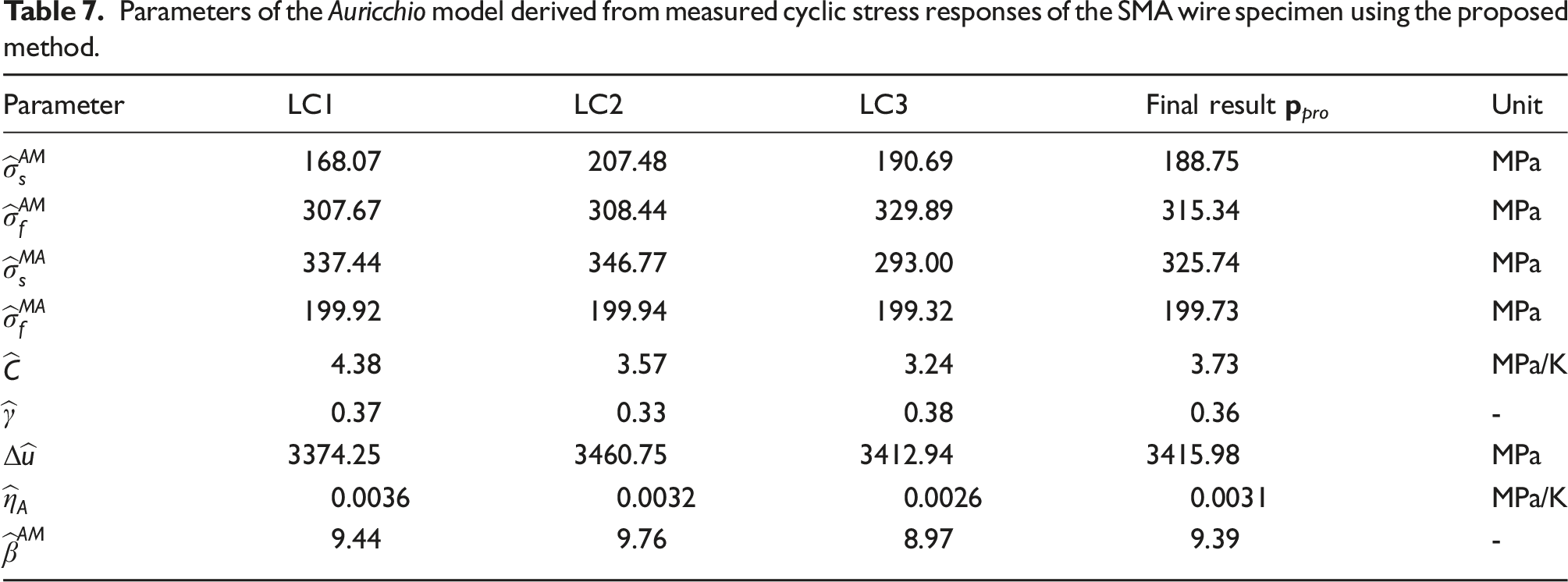
Parameters of the Auricchio model derived from measured cyclic stress responses of the SMA wire specimen using the proposed method.
Furthermore, to validate the accuracy of the identified parameter set, we executed experiments for load cases different from model training, referred to as LC4–LC6 (cf. Table 4). For validation purposes, Figure 8 juxtaposes the measured stress–strain responses with those predicted by the constitutive model using the identified parameters for the load cases LC3 and LC6. These predictions closely mirror the dynamic behavior observed in the experimental results. Comparison of the experimental results (EXP) to the predictions (COM) generated by the Auricchio model using parameter set 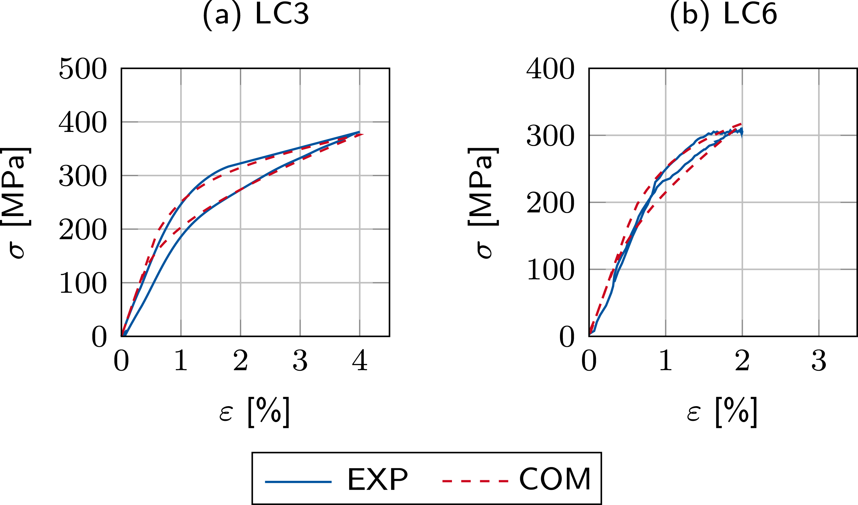
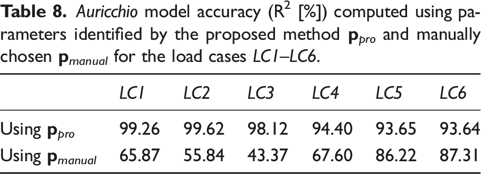
Auricchio model accuracy (R2 [%]) computed using parameters identified by the proposed method
Moreover, to highlight the effectiveness of the methodology, Figure 9 juxtaposes the measured stress–strain responses for the load cases LC3 and LC6 with those predicted by the constitutive model using the identified parameters, where the internal energy change between the austenite and martensite phases is manually determined as Δu = 650.18 MPa. This parameter set is denoted as Comparison of the experimental results (EXP) to the predictions (COM) generated by the Auricchio model using a manually identified parameter set 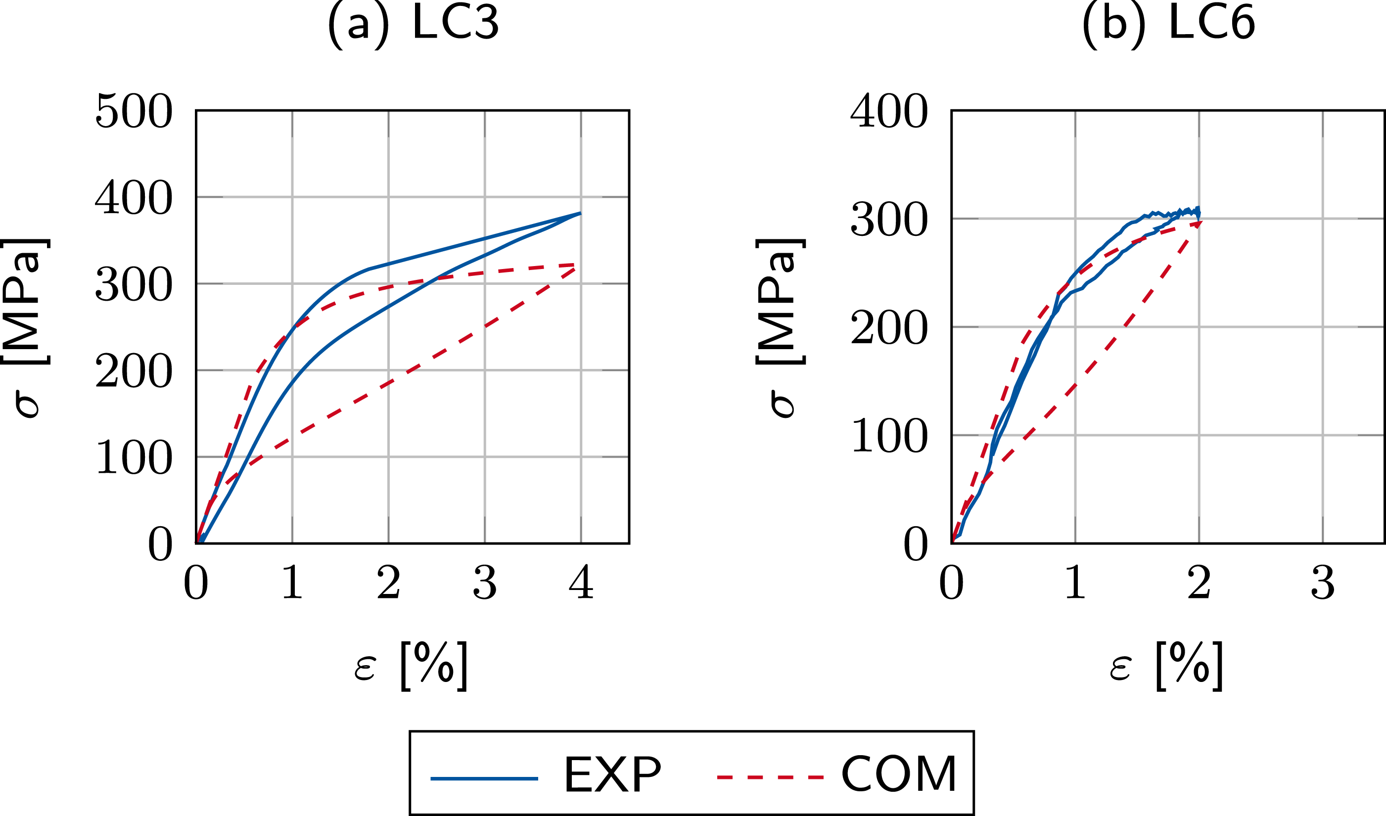
3.2. Zhu and Zhang model
For the Zhu and Zhang model, our objective is to identify the parameters for another Nitinol wire sample with alloy composition Ni-55.90% and Ti-43.95%, manufactured by Baoji Hanz Metal Material Co. The known parameters are as follows: • Young’s modulus-austenite: E
A
= 29,000 MPa • Young’s modulus-martensite: E
M
= 14,100 MPa • Max. inelastic strain at ξ = 1: ɛ
l
= 4.0% • Density: ρ = 6500 kg/m3
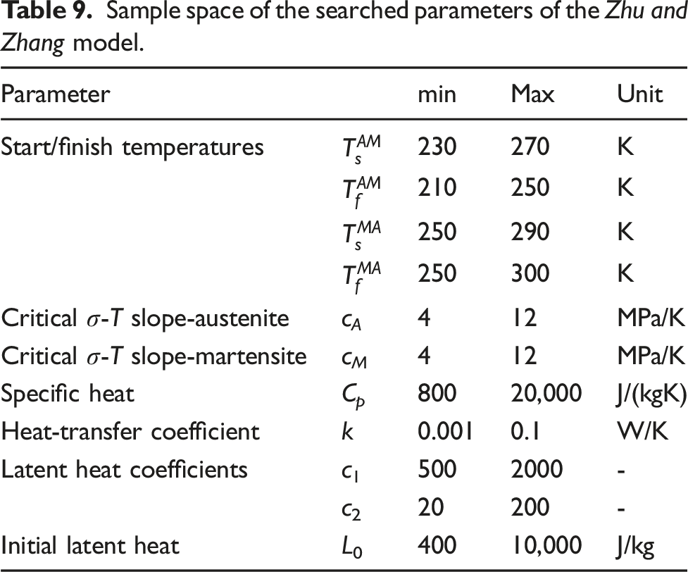
In this case, 11 parameters need to be identified including the four start and finish temperatures
3.2.1. Data generation
Sample space of the searched parameters of the Zhu and Zhang model.
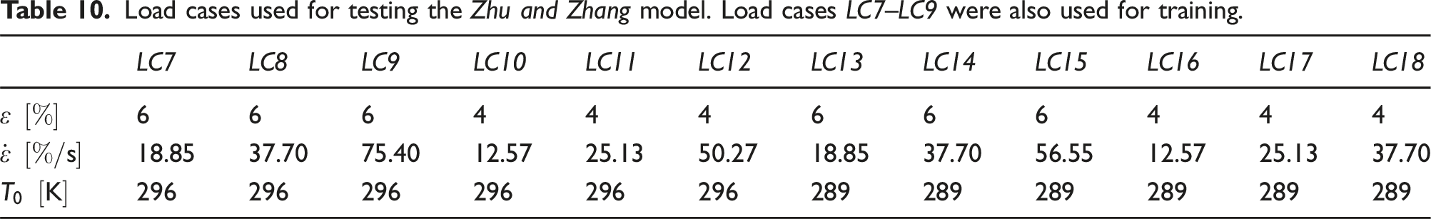
Load cases used for testing the Zhu and Zhang model. Load cases LC7–LC9 were also used for training.
3.2.2.Training
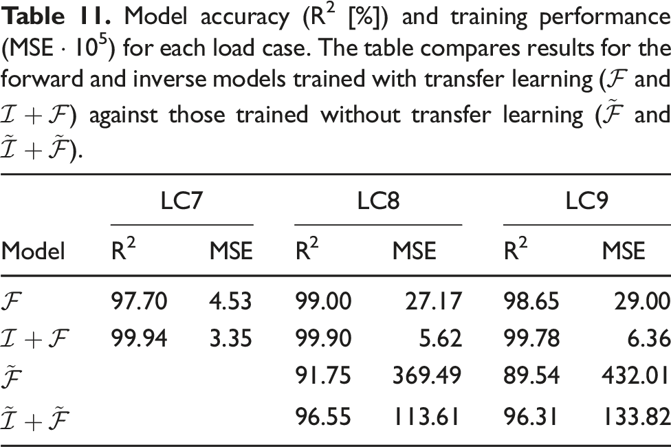
For training, we choose the same architecture as optimized for the Auricchio model consisting of six layers with 100 neurons each. The learning rate is set at η = 1.0 ⋅ 10−3. Moreover, the networks are trained for n e = 2000 epochs using the mini-batch gradient descent method with a batch size of n b = 1000. Beginning with LC7, the training of the forward model is conducted for I = 40 ⋅ 103 parameter combinations. In the next step, the weights and biases of this forward model are saved and utilized for the training of the inverse model. After training the models for LC7, the forward and inverse models corresponding to LC8 and LC9 are trained for n e = 20 epochs, exploiting the weights and biases from the LC7-trained models.
Model accuracy (R2 [%]) and training performance (MSE ⋅ 105) for each load case. The table compares results for the forward and inverse models trained with transfer learning (
3.2.3. Experimental validation
For validation, we conduct stress–strain experiments with the test setup shown in Figure 7 and compare the measurement data with our predictions. In this study, the SMA wire was tested with a length of l = 150 mm and a diameter of D = 0.2 mm. Besides, a pre-stress of σ0 = 139.4 MPa was applied, enabling the desired phase transformation at a strain level that matched the limits of the test setup. Throughout the experiments, the ambient temperature was constant.
Parameters of the Zhu and Zhang model derived from measured cyclic stress responses of the SMA wire specimen using the proposed method.
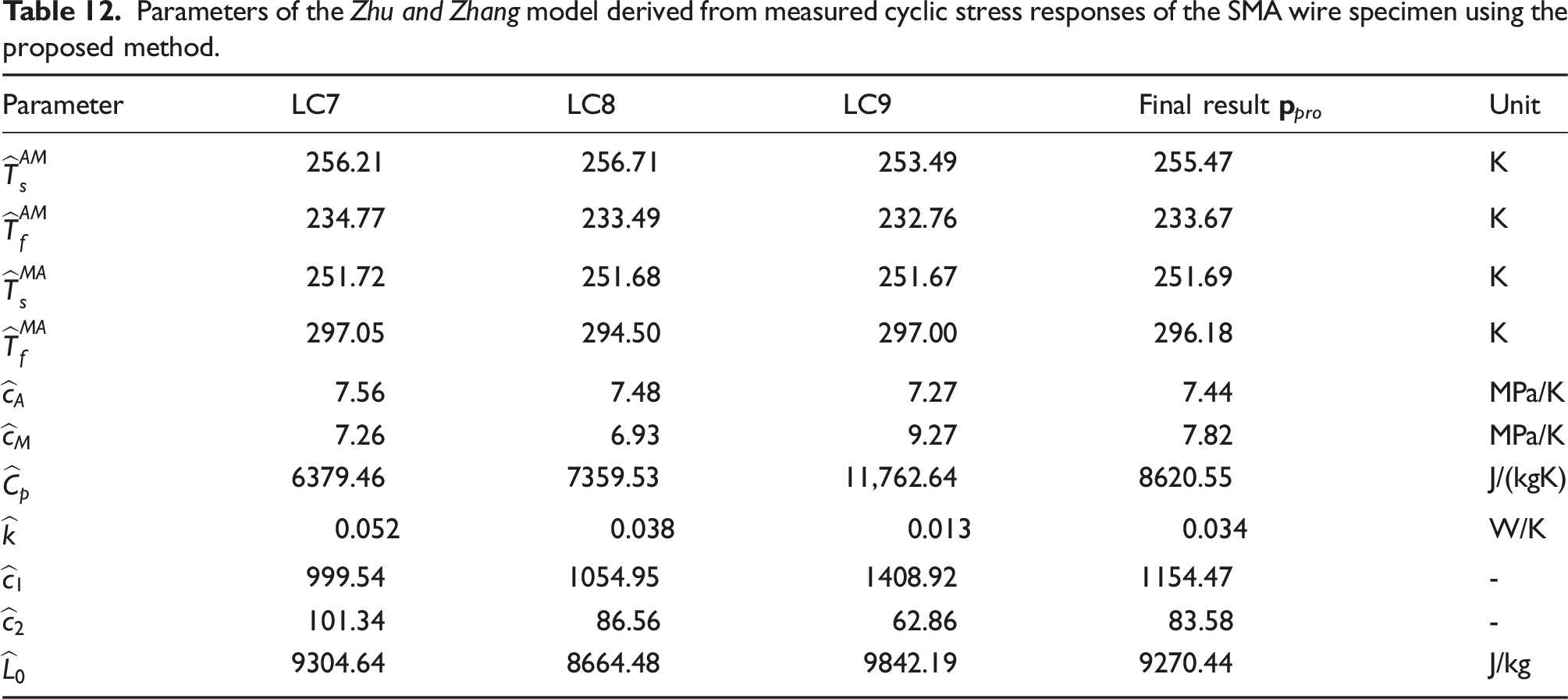
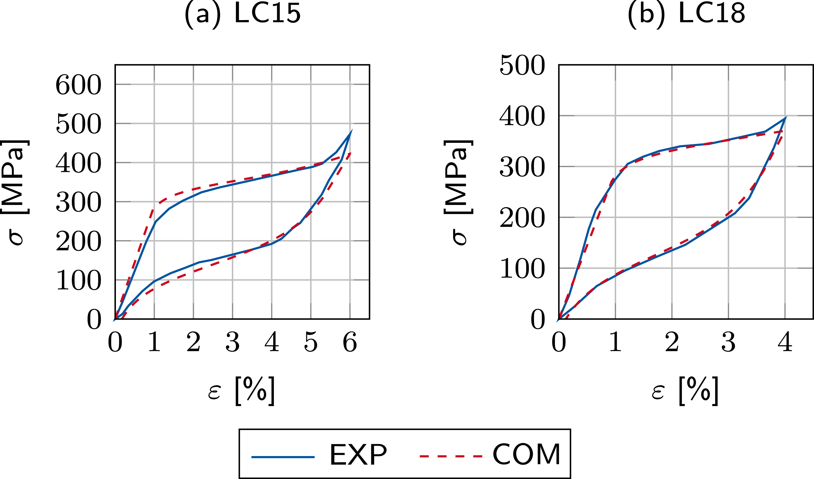
Figure 10 juxtaposes the measured stress–strain responses with those predicted by the Zhu and Zhang model employing the identified parameter set for the load cases LC7 and LC10. Both predictions accurately map the stress–strain behavior of the measurement data. Furthermore, Figure 11 compares the measured stress–strain responses with those predicted by the Zhu and Zhang model using the identified parameter set for the load cases LC15 and LC18. The results show that the constitutive model employing the identified parameter set is able to accurately map the experimental stress–strain behavior even at different ambient temperatures, demonstrating the generality of the parameter set identified by the proposed method. Comparison of the experimental results (EXP) to the predictions (COM) generated by the Zhu and Zhang model using parameter set Comparison of the experimental results (EXP) to the predictions (COM) generated by the Zhu and Zhang model using parameter set 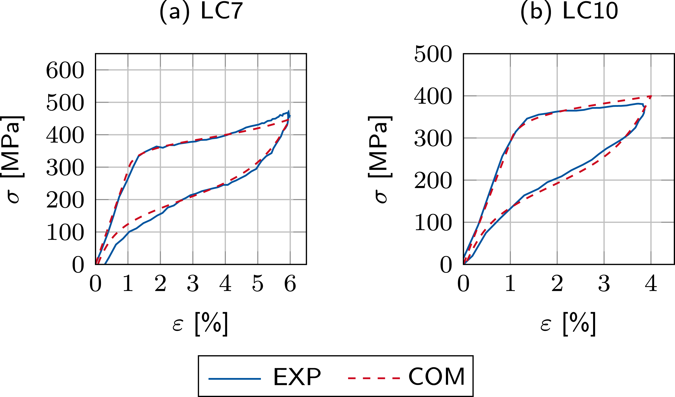
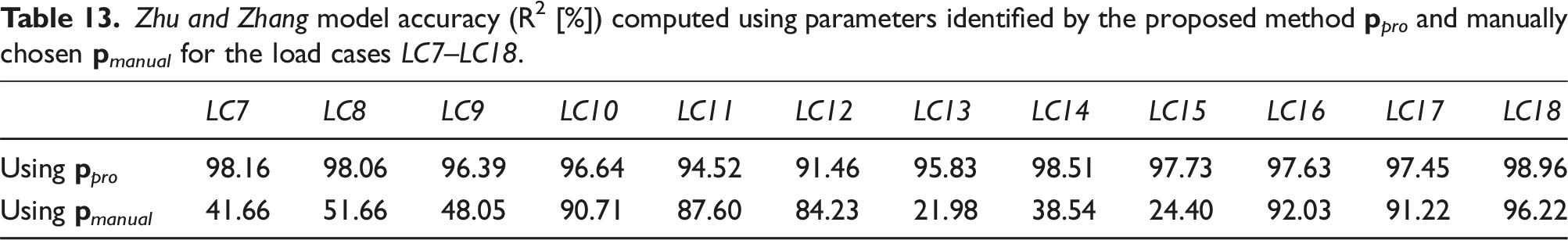
Zhu and Zhang model accuracy (R2 [%]) computed using parameters identified by the proposed method
Additionally, to demonstrate the efficiency of the methodology, Figure 12 compares the measured stress–strain responses for load cases LC7 and LC10 with those predicted by the constitutive model using the identified parameters, where the latent heat coefficient c2 is manually set to c2 = 146.36. This parameter set is denoted as Comparison of the experimental results (EXP) to the predictions (COM) generated by the Zhu and Zhang model using a manually identified parameter set 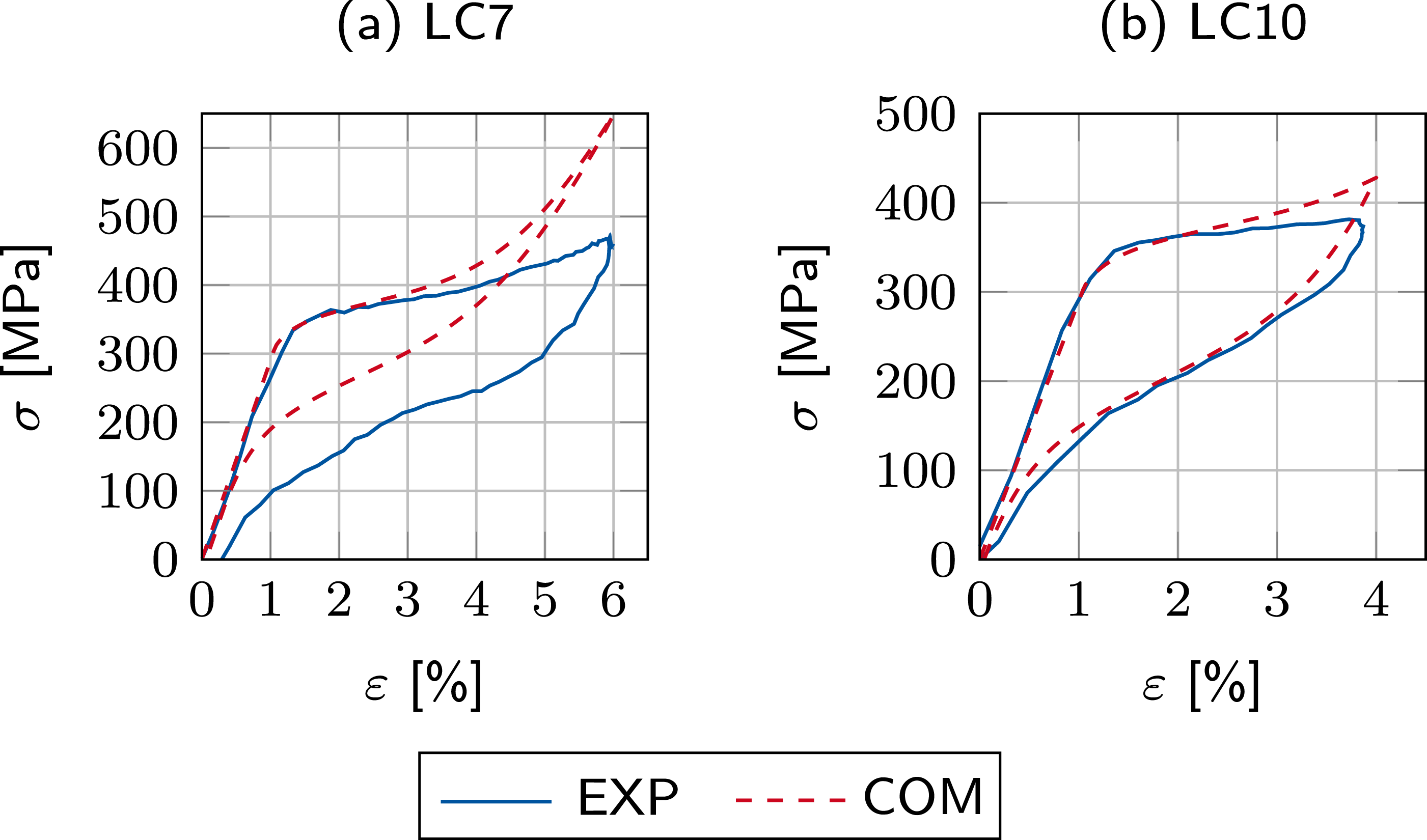
3.3. Application example
To demonstrate the importance of accurately identified model parameters, we use the Auricchio model with the determined model parameter sets Shear frame structure with its degrees of freedom (x
i
for i = 1, 2, 3) and retrofitted with dampers made of SMA wire bundles. The structure faces the challenge of ground acceleration, represented as 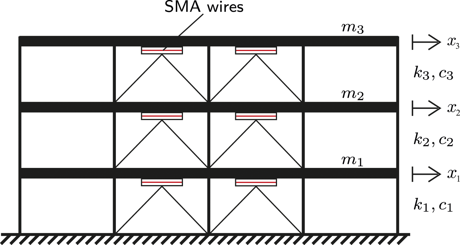
To protect the structure from seismic activities, particularly the historical El Centro, May 1940 earthquake, two dampers made up of SMA wire bundles are envisaged to be affixed between each floor. Designed to operate exclusively under tension, these SMA wires match the properties of the previously identified Nitinol alloy (comprising Ni-55.8% and Ti-43.55%). Each wire bundle spans a length of l = 600 mm and possesses a combined diameter of D = 77.46 mm.
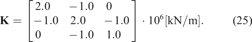
The equation of motion of the structure reads


The structural responses are derived using the Newmark-beta algorithm. In this approach, the restoring force for each damper is calculated based on the stress responses given by the constitutive model, represented as
The time history of the earthquake is shown in Figure 14. In Figure 15, the displacement responses of the third floor are presented, showing both scenarios: with and without the dampers. Here, the displacement responses of the third floor are calculated for both parameter sets: Ground acceleration of the El Centro earthquake applied to the structure. Displacement response on the third floor. The SMA responses are computed using the parameters identified by the proposed method 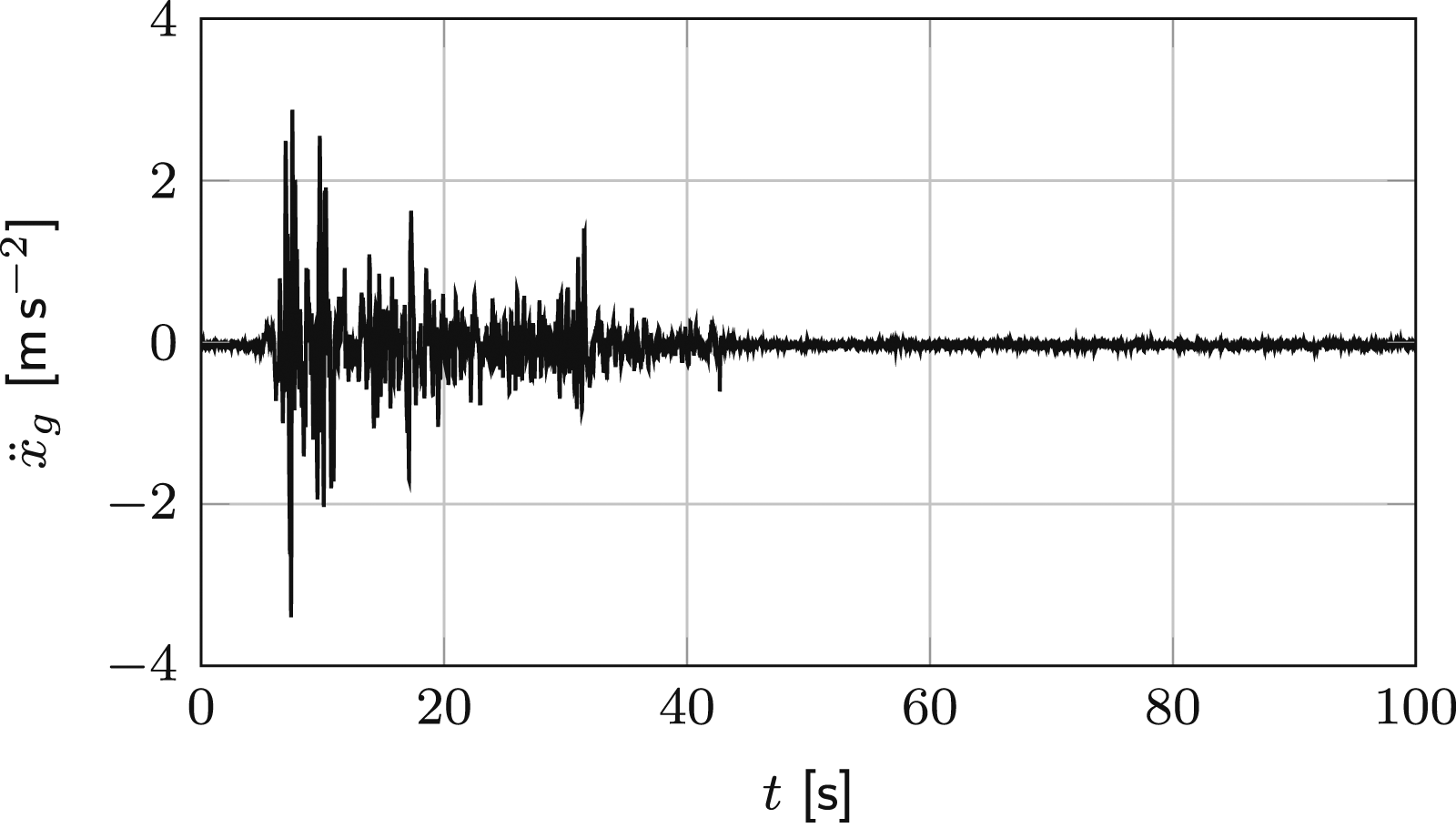
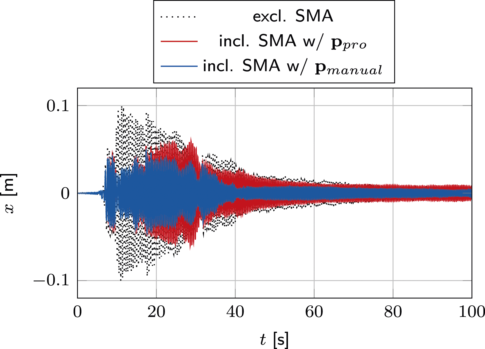
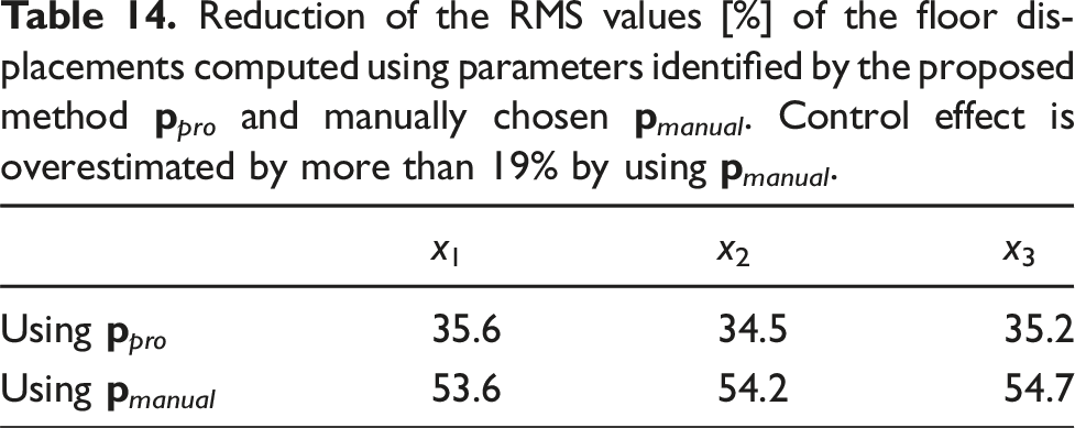
Reduction of the RMS values [%] of the floor displacements computed using parameters identified by the proposed method
4. Conclusions
This paper introduced a method for parameter identification and tuning utilizing FNNs for uniaxial superelastic SMA models under dynamic loading. Given the ill-posed nature of the inverse parameter identification problem, a dual network architecture is used, where a surrogate forward model is paired with the inverse model. Simultaneously, this dual network architecture minimizes reliance on expert knowledge for constitutive model and parameter space selection. The networks are trained to reconstruct the target stresses, ensuring that the constitutive model accurately mimics the material responses, regardless of the physical interpretations of the identified parameters. This coupling benefits from transfer learning, ensuring consistency in parameter sets across various load scenarios. In our case study, we also accelerated the training speed with transfer learning. After an initial training of the first load case for 2000 epochs, only 20 epochs sufficed for the subsequent two load cases. Upon completion of training, the inverse models accurately identified and fine-tuned multiple parameters of two different constitutive models as well as two different SMA wire compositions. Experimental validations using in total 18 load cases including two different ambient temperatures confirmed that, with the identified parameters, the constitutive models reproduced stress responses with high precision, demonstrating generality of the parameter set identified by the proposed method. For the first SMA wire composition, the Auricchio model exceeded an accuracy of 98% for the trained load cases and 93% for the test load cases. Similar accuracy was achieved by the Zhu and Zhang model using a second SMA wire composition, where 96% for the trained load cases and 91% for the test load cases were reached. Furthermore, the application of the method to a numerical example with an SMA-retrofitted structure demonstrated the importance of precisely identified parameter sets. Two scenarios were tested: parameters identified by the proposed method and parameters chosen manually. The results show that even by varying one parameter the responses can be miscalculated significantly.
Looking forward, the study opened several directions for further exploration. While the current study focused on a specific Nitinol, the method is adaptable to other SMA compositions. To achieve this, expansions to the parameter space, including considerations for Young’s moduli and maximum inelastic strain, will be necessary, alongside additional experimental validations. Furthermore, the data in this study catered to a single SMA wire with experiments designed accordingly. However, for SMA bundles, thermodynamic behavior alterations (Casciati et al. (2018)) suggest potential model refinements to enhance accuracy. Experimental validation of such models requires adequate cyclic tensile tests, demanding our test setup to potentially be adapted, such that, for example, thicker SMA wires or bundles can be tested. Lastly, as for other machine learning applications, the training performance of the models depends on the representativeness of the data, which is related in this study to the choice and discretization of the load cases. This aspect deserves further research, such as using methods from active learning.
With continuous advancements in the field of materials science and computational methods, the integration of FNNs with constitutive modeling holds promising potential to discover and harness the unique properties of SMAs in practical applications.
Footnotes
Declaration of conflicting interests
The author(s) declared no potential conflicts of interest with respect to the research, authorship, and/or publication of this article.
Funding
The author(s) received no financial support for the research, authorship, and/or publication of this article.