
Abstract
With the intention to detect structural events, for example, occurrence of damage and assessing their severity under service, structural health and event monitoring proved itself as a reliable evaluation tool. While many algorithmic approaches exist, model-based monitoring offers the prominent advantage to enable extensive analysis of damage states based on a structural digital twin. In order to accurately replicate the dynamical behaviour of a real-world structure, inherent physical properties, for example, mass, stiffness and structural damping, of the digital twin might be corrected from nominal values. This can be achieved by numerical model updating procedures. In this study, the application of a model updating approach is presented to eliminate modal discrepancies. Based on the perturbated modal dynamic residual, an updating equation is formulated. Stiffness and mass correction terms with preserved orthogonality and symmetry conditions are determined by the method of least squares. A case study using computationally generated modal data is conducted, evaluating the numerical updating performance in terms of correction accuracy and reproduction of modal parameters. Finally, the transient structural response to an impulse excitation is compared between updated and reference model. The gathered results prove the method’s suitability as accurate and robust updating procedure, fostering its application in model-based monitoring frameworks.
1. Introduction
With advances in sensor technology and data-driven analysis, the concept of structural health and event monitoring (SHEM) has become of major importance to various engineering disciplines over the last decade in civil, military, aerospace and automotive applications (Balageas et al., 2016; Haidarpour and Tee, 2020). Enabling an almost real-time, full-scale evaluation of the structural integrity without interrupting operation cycles, an embedded monitoring system can be understood as a non-destructive evaluation technique (NDE). This enables condition-based maintenance and eliminates the need to interrupt operations for inspection. In the very special case of aerospace applications, neither manual inspection nor maintenance might be possible at all. However, mission success depends on the structural reliability of spacecraft components and demands early detection of potential issues to prevent catastrophic failures.
According to Beard et al. (2005), SHEM systems consist of three similar components: (1) A permanently attached or embedded sensor/actuator network, (2) a data acquisition system (DAQ) with potential preprocessing capabilities and (3) a data processing unit (DPU). The DPU, considered the core of each SHEM system, is tasked with extracting meaningful features from large, complex datasets to detect singular events, such as sudden impacts or the evolution of fatigue, before they threaten operational safety. However, the success of these predictions relies heavily on the chosen algorithm, making the appropriate selection of the approach crucial, as the high volume and complexity of the data make analysis challenging. Further information on monitoring strategies can be found in Figueiredo et al. (2009), Haynes (2014), Sun and Qin (2014), and Yang et al. (2014). Algorithmic approaches allow distinction between data-driven and model-based methodologies (Fan and Qiao, 2011; Vagnoli et al., 2001; Worden and Manson, 2007). Some authors offer other differentiations, for example, local versus global (Balageas et al., 2016) and linear versus nonlinear (Haidarpour and Tee, 2020), but are beyond the scope of this paper.
From the operator’s perspective, model-based monitoring allows comprehensive understanding of the system’s structural condition. This offers a superior advantage over data-driven analysis but requires a highly sophisticated model. Implementing such structural model can be challenging as it necessitates a thorough understanding of the system’s physical properties and environmental interactions. If not all relevant information is accessible, the implementation of such a mature model can be problematic even with expertise. In this case, numerical model updating (NMU) techniques can be utilized to improve the accuracy of the model and ultimately enhance the reliability of the monitoring results (Friswell and Mottershead, 1995). NMU has gained broad attention within SHEM applications since it allows deriving high-fidelity baseline models for model-based health monitoring. Once such a digital twin is implemented, NMU allows structural damage identification by various methods which were reviewed from Sharry et al. (2022).
2. Delimitation to existing methods
In this study, mass and stiffness updating is considered. Numerous prior research efforts have been dedicated to this approach. Similar to this study, their updating equations minimize the modal dynamic residual and enforce orthogonality resp. symmetry constraints. Thus, the derivation of the hereinafter investigated updating procedure might be partially similar to existing methods mentioned below. The following section summarizes prior research efforts that are most closely related to the present study.
In the late 1980s, first proposals for individual mass or stiffness updating have been published by Baruch and Itzhack (1978) followed by Berman (1979). They introduced modal based updating for either mass or stiffness matrix while assuming sufficient accuracy for the remainder. Baruch (1982) proposed an early approach to correct the system matrices sequentially by formulating two different updating variations based on the assumption that either system’s mass or stiffness is known with higher confidence. Caesar and Peter (1998) derived a generalized linear least square formulation for individual mass and stiffness updating with included symmetry, orthogonality and additional force equilibrium constraints. However, considering the matrices’ interdependent nature towards the modal dynamic residual, the practitioner is challenged to decide on the more accurate property while limiting the full updating potential as one matrix remains unaltered during each updating step. Consequently, a simultaneous updating methodology for both mass and stiffness should be favoured.
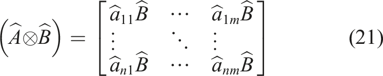
Sarmadi et al. (2016) expanded the mass and stiffness orthogonality based on the dynamic discrepancy theory, establishing two improved updating formulations to determine correction terms as discrepancy matrices. Similar to this study, they transformed the updating formulation into a non-square linear equation system using the Kronecker tensor product (see (21)) and determined the solution by iterative methods. However, their methodology does not facilitate the removal of constrained and sparse matrix entries which becomes a notable drawback when dealing with large-scale systems.
Iterative methods, as the one presented in this study, often incorporate the modal dynamic residual or the frequency response function (FRF) as part of their objective function. Arora (2011) investigated the achieved updating accuracy in terms of the obtained frequency response function (FRF) when applying direct or iterative updating approaches. Dong and Wang (2016) evaluated the frequency domain updating performance of two different updating procedures where one approach involves the minimization of the modal dynamic residual. They also compared different iterative solvers to find suitable updating parameters for the system’s stiffness matrix. Li et al. (2018) investigated the structural identification process for stiffness correction, utilizing the modal dynamic residual approach which was minimized by LSQR (least squares method). In their study, they also compared the performance of different gradient-based solvers. Based on this, Li and Wang (2019) also addressed the problem of unfeasible computational efforts when dealing with large datasets. Similar to this study, they exploited sparsity to significantly reduce the size of the optimization problem. However, FRF-based updating formulations are constrained by their inability to target individual modes or eigenfrequencies for updating. Instead, they update the entire frequency spectrum captured by the FRF. The lack of granularity in selecting particular modes or eigenfrequencies limits practitioners seeking to fine-tune specific dynamic characteristics of their structures.
Further studies investigated the application of stochastic and metaheuristic optimization such as evolutionary algorithms (EA) for model updating. Gomes et al. (2018) provided a comprehensive review of vibration-based inverse techniques for damage detection and identification which included FE model updating by genetic algorithms (GA), swarm optimization, etc. They also summarized objective functions which were assembled from modal parameters such as natural frequencies, mode shapes or FRF of the reviewed studies. Jafarkhani and Sami (2011) evaluated the updating performance of stochastic optimization algorithms for finite element model updating to monitor dispersed civil infrastructures. The damage detection results revealed fair agreement between the qualitative reported visual inspections and identified damages through model updating, proving the potential of EA for model-based health monitoring. Another real-world application was demonstrated by Sun et al. (2020), using a two-phased updating technique to assess the mechanical state of an in-service cable-stayed bridge by GA which significantly improved FE model accuracy. However, as those metaheuristic approaches can be powerful for global optimization and exploring complex solution spaces, they demand high computational costs when dealing with large parameter spaces. As in direct mass and stiffness matrix updating every non-sparse matrix entry can be considered an optimization parameter, the parameter space expands rapidly and makes evolutionary algorithms suffer from slow convergence. On the contrary and as proposed in this study, gradient-based methods leverage the gradient information to iteratively refine the algorithmic parameters in a more adaptive manner which often leads to faster convergence.
This study presents a methodology for simultaneously updating of mass matrix M and stiffness matrix K of a structural FE model by correction terms ΔM and ΔK to reproduce set of modal parameters (specific eigenfrequencies ω and mode shapes ϕ). The updating procedure is derived by perturbating the modal dynamic residual which is minimized by a gradient-based solver. The updating equations account for orthogonality and symmetry constraints, exploit sparsity patterns to deal with large datasets and allow to precisely target specific modal sets within the updating objective. Ultimately, a straightforward formulation allows convenient implementation for the practitioner while its high correction accuracy encourages confident application in real-world scenarios.
3. Updating methodology
In structural dynamics, the behaviour of a structure subjected to dynamic loads can be described by second-order ordinary differential equations as follows:


To examine the structure’s natural vibrational characteristics, (1) is further simplified by neglecting damping forces and external loading. Assuming the stationary solution


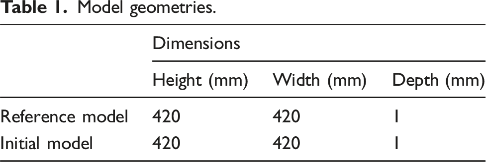
To introduce the updating procedure, subscripts indicate the affiliation to different models: Firstly, a reference model (RM) shall be labelled by the subscript R. The RM’s structural properties are known in advance and serve as benchmark to evaluate the updating performance. Secondly, an initial model (IM) with yet unknown parameters is identified by subscript I. The purpose of the latter is to reproduce the RM’s modal parameters based on correction terms ΔK and ΔM as a solution to the updating equation.
With the assembled mass and stiffness matrices from the IM M
I
,

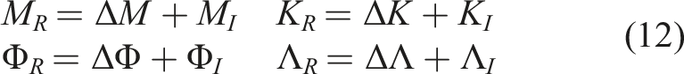
Usually, m ≪ n holds true since the considered set of modal parameters represents only a small subset to the solution space of (11). In a real-world updating scenario, only M R and K R remain unknown since Φ R and Λ R can be determined by experimental modal analysis (EMA) of the examined structure. Including all correction terms (12) into the modal dynamic residual (11) yields different updating formulations: Either solely updating of stiffness by ΔK or simultaneous updating of both mass and stiffness by ΔM and ΔK. In the following, both approaches are introduced in Section 3.1 and Section 3.2, and the reader can directly skip to the desired chapter based on their updating preference. Isolated updating of M might be possible as well following the procedure in Section 3.1. However, several authors suggest to neglect isolated mass matrix updating since assembling from nominal material properties achieves sufficient accuracy (Halevi et al., 2003).
3.1. Isolated updating of stiffness matrix
For the purpose of isolated updating of stiffness matrix K, mass correction ΔM is disregarded from the modal dynamic residual (11):
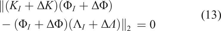
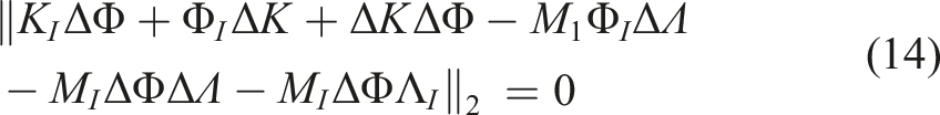
Finally, separation of the correction term ΔK leads to the following equation:
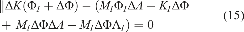
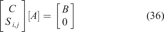
At this point, matrix norm ‖ ⋅‖2 is neglected for improved readability even though mapping matrix–vector terms to scalar quantities is only applicable when applying matrix norms. Finally, (15) can be reshaped to a linear equation system:


To solve for matrix A resp. ΔK, rearrangement of (16) is required. This can be achieved by the following expression:
Due to the incomplete solution set Φ
I
, Λ
I
to the modal dynamic residual (11),

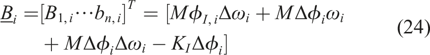

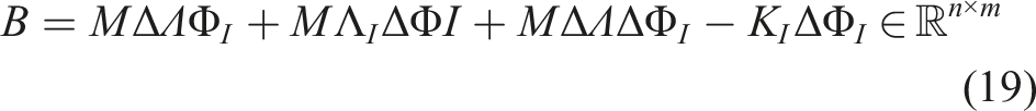
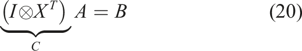
To clarify, terms A and B of (20) are described by (25) and (24) while C is assembled by (23) when isolated updating of stiffness matrix K is foreseen.
3.2. Simultaneous updating of mass matrix and stiffness matrix
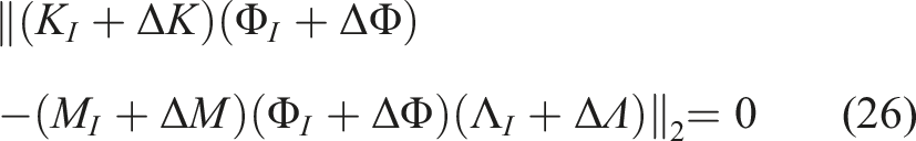
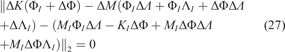
This section introduces the updating equation for simultaneous updating of stiffness matrix K and mass matrix M based on the same perturbation approach as in Section 3.1. As an entry point, the modal dynamic residual (11) with correction terms including ΔM and ΔK is considered:


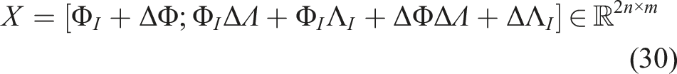
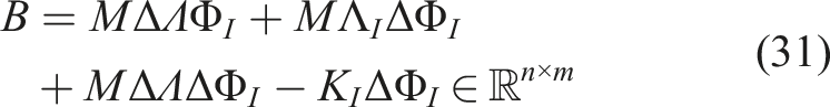
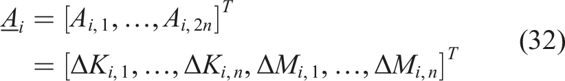
Again, a rearrangement is required to solve for A as stated in (20). This time, A consists of vectors
Since
3.3. Including matrix symmetry conditions
So far, the updating equations do not comply with symmetry conditions. For symmetric correction terms, the symmetry constraints


The vector
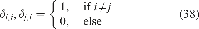
The modification denotes the Kronecker delta’s inverted properties which is equal to 1 − δi,j. By assigning i, j to all non-zero matrix elements for each
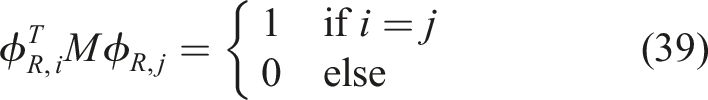
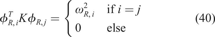
3.4. Including mass and stiffness orthogonality
A similar approach can be adopted to achieve mass and stiffness orthogonality regarding the modal set Φ
R
, Λ
R
. For mass orthonormal modes, the orthogonality constraints
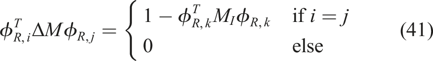
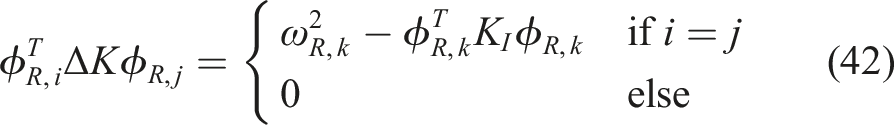
Since ΔM and ΔK are square matrices, (41) and (42) can be included into (20) by
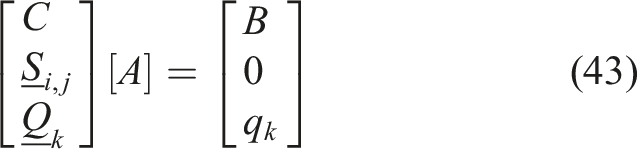

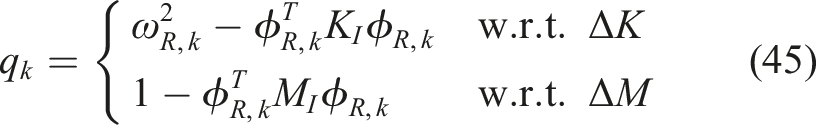
The symmetry constraints (36) are already included in (44) for the sake of completeness. To demand orthogonality of pairing modes, q
k
can be set to
3.5. Additional constraints
Further constraints can be considered by excluding specific matrix elements from the updating procedure. This applies to, for example, fixed single point constraints in terms of translation and rotation or zero-elements of M and K whose altering would generate non-existent stiffness and mass coupling. Therefore, all corresponding rows of A and columns of terms C,
3.6. Solving as optimization problem
Finally, the updating equation allows determining correction terms ΔM and ΔK to given mass and stiffness matrices M
I
and K
I
such that the modal subset Λ
R
, Φ
R
is reproduced. This can be summarized in the unconstrained optimization problem:

Under consideration of symmetry (35) and orthogonality constraints (39) and (40), the non-square linear equation system (20) optionally with (36) and (43) is solved instead.

4. Numerical investigation
Model geometries.
4.1. Correlation metrics
In this study, different modal and time domain correlation tools are used to identify discrepancies in the dynamic structural response. Those are listed in the following with the introduced notation for IM and RM:
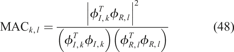
According to Pástor et al. (2012), MAC is sensitive to nodal DOFs with large modal displacements and tends to neglect minor mode shape deviations which might contribute to a decrease of correlation. Therefore, it should be mainly used for global mode shape comparison instead of local correspondence assessment.

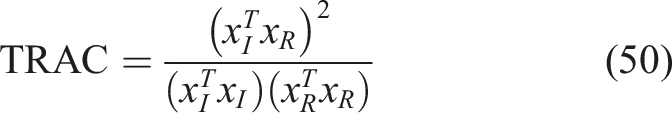
According to Reyes et al. (2017), TRAC can be understood as a regression analysis with the TRAC value being the R2 coefficient.
4.2. Simulative setup
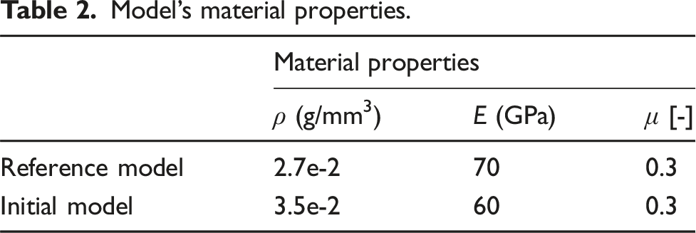
Model’s material properties.
Modelling is realized by solid second-order hexahedral elements as standard volume elements of this study. Despite the fact that thin-walled structures may be more efficiently modelled with structural plate or shell elements, standard elements are used to emphasize the updating procedure’s versatility independent of element type constraints. It is noteworthy to mention that different element types, global mesh refinement, etc., will introduce variations in mass and stiffness matrix entry’s magnitude. However, the updating formulation remains unaltered since core assumptions, that is, matrix symmetry and orthogonality, persist despite the choice of modelling. As this study is intended to investigate the updating performance on a general simplified structural model with uniform material and mesh properties, effects of advanced modelling techniques, for example, non-uniform material/mesh partitioning, are not covered in the numerical analysis.
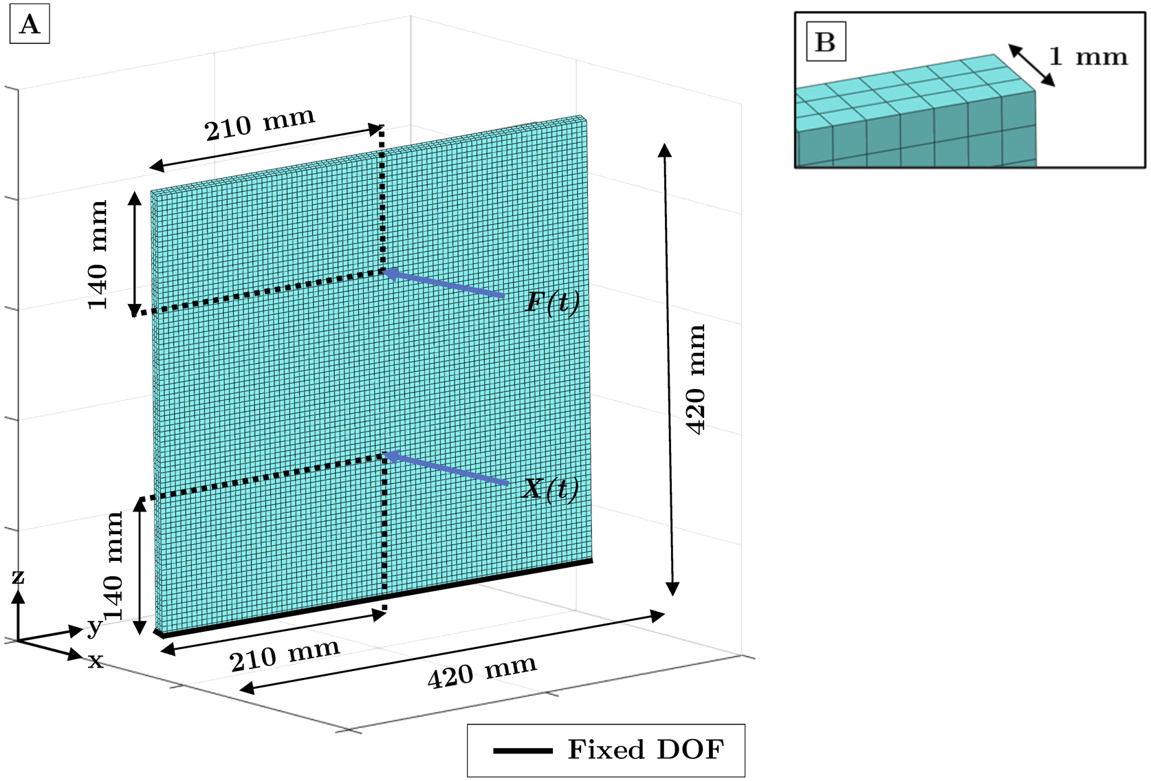
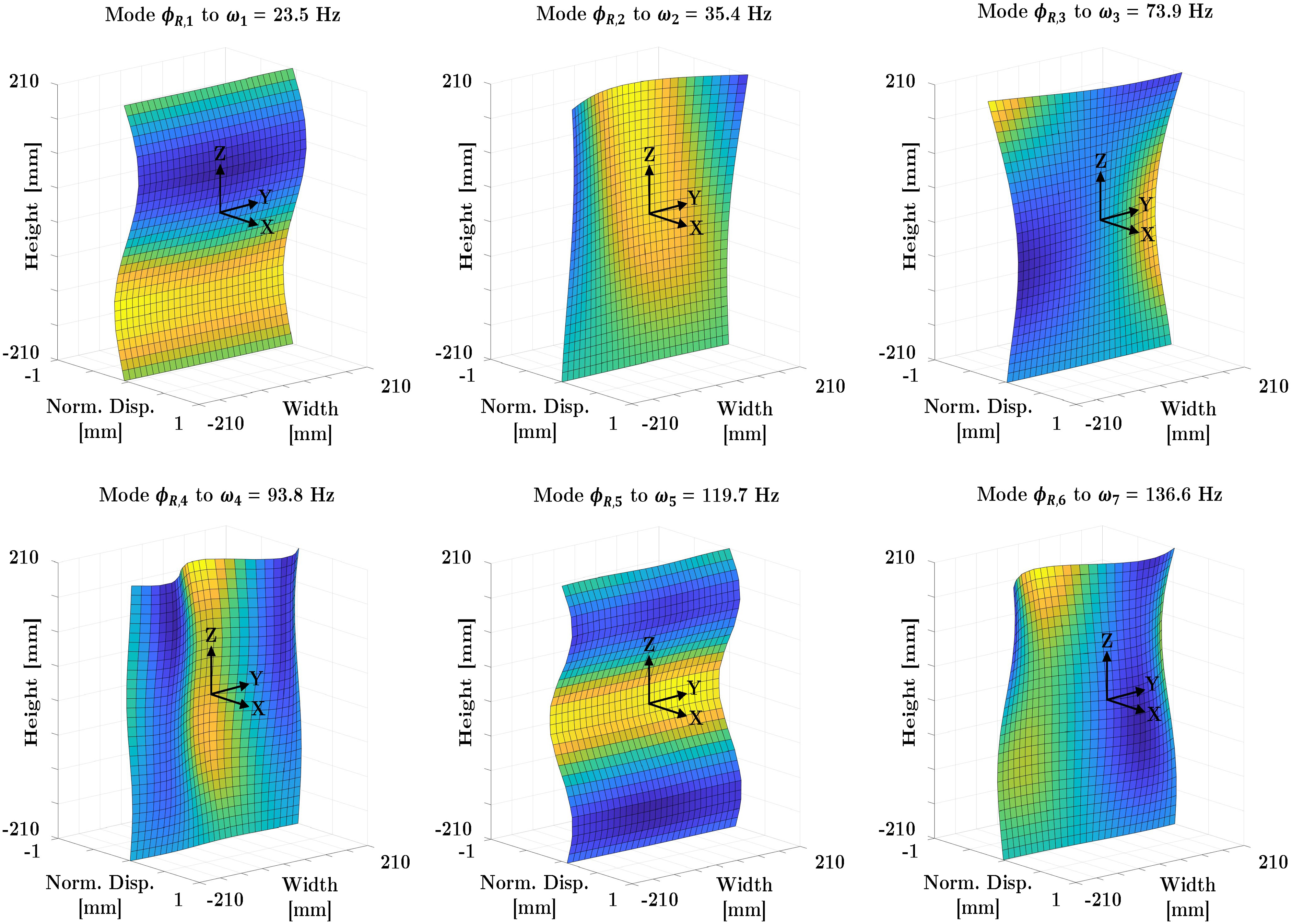
The described numerical setup and boundary conditions, resulting from the clamping at the specimen’s bottom edges, are illustrated in Figure 1. Additionally, the resulting mode shapes Φ
R
and eigenfrequencies ω
R
of the RM are displayed in Figure 2. The updated IM’s matrices and modal properties are labelled by (*) as Description of the numerical setup. Subfigure (a): Illustration of cantilever plate’s FE mesh with dimensions, boundary conditions, measurement point X(t) and excitation point F(t). Subfigure (b): Cantilever plate’s depth. Normalized mode shapes Φ
R
and eigenfrequencies ω
R
of the RM from 1st to 6th mode. For the purpose of illustration, the modal displacements are normalized and scaled.
In the following, Section 4.3, Section 4.4 and Section 4.5 are dedicated to answer those questions. In order to examine Question 1, the modal subset Φ R , Λ R of RM and updated IM are compared. To evaluate their modal correlation, both MAC and CoMAC are used. Additionally, preservation of mass and stiffness orthogonality after updating are investigated. To evaluate Question 2, the Percentage Error of mass matrix and stiffness matrix elements are analyzed by the empirical cumulative distribution function. Regarding Question 3, an impulse response of the updated IM’s is compared to the RM. The response is measured as nodal acceleration from measurement point X(t). To induce vibrations, an impact event is simplified by an impulse function F(t) applied to an excitation point as nodal force. The modelling of the impulse excitation function is described in Section 4.5. TRAC is used to examine the time domain data correlation. Additionally, the power spectral density (PSD) is computed to allow comparison in the frequency domain.
4.3. Question 1: Reconstruction of modal parameters
Comparison of eigenfrequencies.
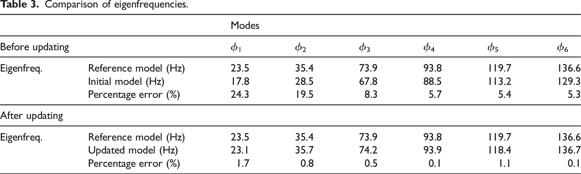
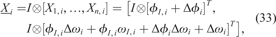
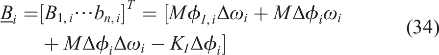
Before updating, considerable discrepancies appear throughout the examined eigenfrequency spectrum, resulting in percentage errors ranging from approx. 5−25%. The lower modes, such as the 1st and 2nd modes, tend to have larger eigenfrequency deviations with errors of 19.5−24.3%. In contrast, 4th to 6th modes remain with similar errors at 5.3−5.7%. After the updating, the eigenfrequencies of IM and RM closely match across the considered frequency spectrum. The diminished eigenfrequency deviations result in percentage errors below 2%. The highest deviation of 1.7% is found again in the fundamental mode. The tendency of enforcing high-order modes to be more accurate might be explained by (33) and (34) since the included eigenfrequency difference Δω i acts as natural weighting factor for high-frequency content. Although the purpose of this unintentional weighting might be questioned, it proves to have a meaningful consequence since higher modes are more prominent in the dynamical acceleration response which are usually measured by acceleration signals. Lower modes, on the other hand, dominantly participate in the overall dynamical response. Therefore, this eigenfrequency weighting gives balanced attention to both high and low frequency content. Depending on the included modes within the updating procedure, this balancing will eventually suffer and demand additional compensation weights. The magnitude of this compensation might be customized for the individual application.
The correlation of the updated IM’s mode shapes Mode shape correlations from updated IM’s mode shapes 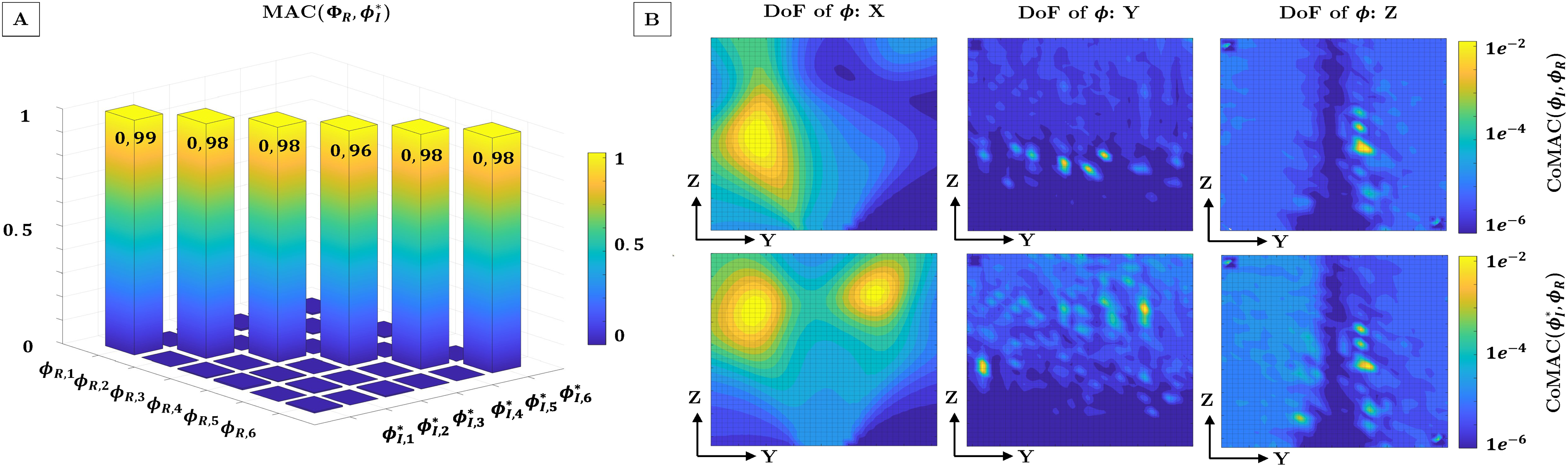
The results of subtracting 1 − CoMAC and projecting onto the mode shapes before and after updating are compared in Figure 3, Subfigure B. It can be seen that correlation properties of DOFs in X-direction are mainly affected. Before the updating process, most uncorrelated nodes are distributed around a pole in the plate’s left centre half. Afterwards, nodal correlation properties evolve into a more axisymmetric shape and split into separated poles in the plate’s upper region. For both Y- and Z-direction, CoMAC values remain almost unchanged. The maximum value of 1 − CoMAC doesn’t exceed 1e-2 for X, Y- and Z-direction which indicates high nodal mode shape correspondence. Therefore, no severe decrease of nodal correlation is apparent.
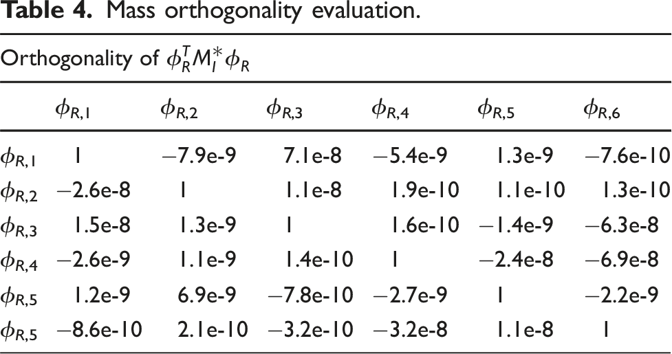
Mass orthogonality evaluation.
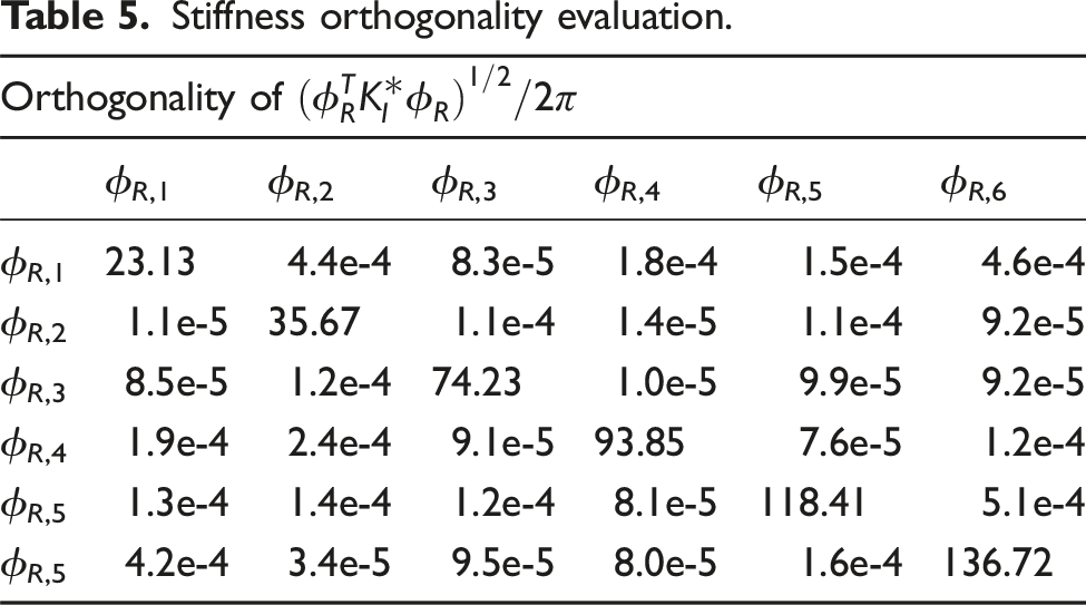
Stiffness orthogonality evaluation.
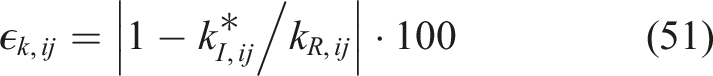
4.4. Question 2: Accuracy performance of correction terms
Special attention must be placed at the deviations of updated IM’s
In Figure 4, the percentage error distributions and their empirical cumulative distribution function (ECDF) for mass and stiffness are displayed. It can be seen that the majority of percentage errors remains in the lowest error bin of observed values. In fact, the number of low-order errors exceeds high error terms by several magnitudes of order, resulting in an ECDF ≥0.99 after the first histogram bin of ϵ
M
= 1.75e-6 resp. ϵ
K
= 2.5e-5. The maximum error does not exceed ϵ
M
= 5e-5 resp. ϵ
K
= 7 × 10⁻⁴. As a conclusion, the updating procedure determined accurate correction terms ΔK and ΔM. Percentage Error ϵ
ij
evaluation from updated K, M. Subfigure (a) and Subfigure (b): Distribution of ϵK,ij and ϵM,ij for all non-zero entries. Additionally, the empirical cumulative distribution function is computed indicating low percentage errors ϵ
ij
, that is, high updating accuracy.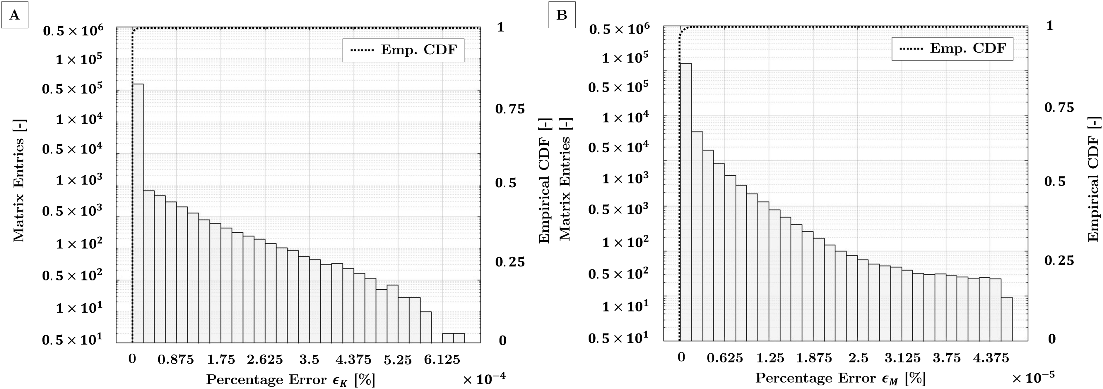
4.5. Question 3: Transient structural response
Finally, the updated IM’s capability to reproduce time domain data is investigated. This is accomplished by applying a nodal impulse excitation F(t) function with force amplitude of 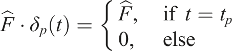
Both impact location and measurement location are depicted in Figure 1. The impact site is situated at the centre of the plate, 140 mm away from the unclamped top edge, while the nodal acceleration
The acquired time domain data is shown in Figure 5, Subfigure A and Subfigure B. In upper Subfigure A, it can be seen that the dynamic response of the IM lacks from lower acceleration amplitudes compared to the RM. This was expected, since the IM was implemented with higher density and lower stiffness (see Table 2). The correlation of nodal acceleration at the measurement point is quantified by TRAC = 0.37. Therefore, the computed impulse response of IM and RM only corresponds to a minor extent. In lower Subfigure A, the nodal acceleration of the updated IM can be seen. The updated IM and RM reveal a high correlation in their dynamic response, resulting in TRAC = 0.79. It can be seen that the time domain correlation has improved significantly but not full correspondence of TRAC → 1 is achieved. This is due to the fact that only a small subset of six modes was incorporated into the updating procedure. However, this improvement is expected to be even higher when the included modal subset is expanded. Comparison of the transient dynamic response to an impulse excitation F(t) measured at the measurement point X(t). Subfigure (a): Nodal acceleration from IM, RM and updated IM* and RM. Subfigure (b): Power spectral density (PSD) of nodal acceleration from IM, RM and updated IM* and RM. For computing the PSD, only acceleration data after impulse excitation t > t
p
is considered.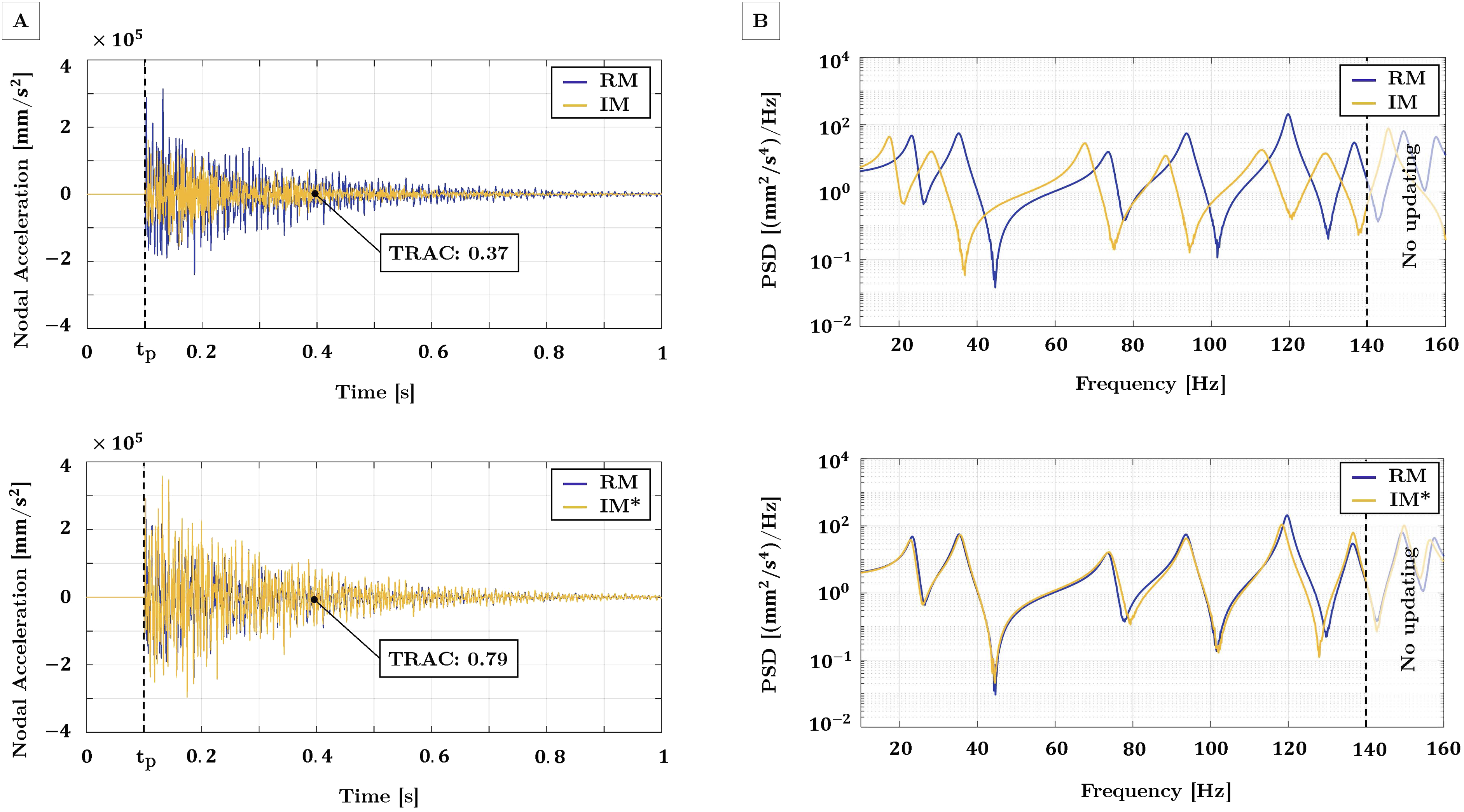
The computed power spectral densities (PSDs) before and after updating are displayed in Subfigure B. In both PSD plots, the relevant frequency spectrum up to the 6th mode is highlighted. As visualized in upper Subfigure B and discussed in Section 4.3, the eigenfrequencies – localized at the spectral power peaks – of the IM strongly differ from the RM. Additionally, the distributed spectral energy shows considerable differences at most of the eigenfrequencies. This corresponds to the observed lower acceleration amplitudes of the IM in Subfigure A. On the contrary, the comparison of PSD from updated IM against RM in lower Subfigure B reveals a high correlation in both eigenfrequencies and spectral power curve. Small deviations in the PSD can be observed at the anti-resonances. However, these discrepancies are of minor relevance for the generated structural response. Consequently, both time and frequency domain data of the updated IM show high correlation to the RM and can be utilized for model-based SHEM frameworks.
5. Conclusion
Structural health and event monitoring (SHEM) has proven maturity in a broad field of industrial applications to assess the structural integrity in the aftermath of singular events, environmental changes and material degradation. To allow model-based SHEM approaches, a high-fidelity structural model is necessary. This can be achieved by numerical model updating (NMU) techniques. In this study, a perturbation-based NMU procedure is investigated to reproduce a modal subset. Balancing the modal dynamic residual and incorporating orthogonality and symmetry constraints allows to derive a non-square linear equation system. Minimizing its residual by any suitable optimization method, for example, LSQR, allows determination of the correction terms. The approach allows including modes of arbitrary number in any frequency regime.
An FE model of an aluminium cantilever plate is utilized for evaluating the updating performance. The model is implemented twice with different material properties as reference model (RM) and initial model (IM). The IM is updated on behalf of the first six modes. The updating procedure determined highly accurate correction terms, allowing to reproduce the RM’s eigenfrequencies within an error margin of 2%. The mode shape correlation was evaluated by the Modal Assurance Criterion (MAC) and the Coordinate Modal Assurance Criterion (CoMAC). Both MAC and CoMAC proved high mode shape correlation between updated IM’s and RM’s modes. Lastly, a transient response to a nodal impulse excitation was computed for updated IM and RM. Time and frequency domain characteristics were evaluated by Test Response Assurance Criteria (TRAC) and Power Spectral Density (PSD). Again, the updated IM was able to reproduce the RM’s dynamic structural response in both time and frequency domain.
While the obtained results encourage to apply the updating procedure to real-world SHEM scenarios, further questions of more practical nature might arise which have not been covered in this study: • The generation of spurious modes can’t be ruled out. This might happen if neighbouring updating modes are far separated, increasing the chance of spurious mode appearance in the frequency gap. Additionally, modes above the considered frequency spectrum might be altered as well. To suppress spurious mode generation, all included modes should be densely packed with regard to their eigenfrequencies. A subsequent correlation check, for example, by MAC to identify spurious modes seems reasonable. • The updating formulation does not allow handling non-nominal constraints resp. boundary conditions as the related DOFs are fully removed from the updating procedure (see Section 3.5). Including those constraint DOFs can be considered fully unlocking of restrictions resp. supports and might enable physically unmeaningful solutions. Additionally, real-world constraints might be subject to more complex phenomena and cannot be sufficiently represented by altering local inertia and/or elastic properties of the structural model. • As more complex structural models resp. geometries require varied element types, material and/or mesh partitioning, mass and stiffness matrices sparsity pattern might be affected and matrix entries with discrepancies in magnitude arise. The latter eventually impacts the condition number of matrix updating equations, causing both the eigenvalue problem and the updating formulation to become sensitive to perturbations in the input data and compromise numerical stability. As this becomes particularly critical when relying on experimentally gathered modal data under less controllable environments, inaccuracies from the measurement setup resp. sensor noise potentially amplify numerical instability of the updating procedure. This might lead to erroneous results that do not accurately represent the actual structural behaviour. To mitigate effects of ill-conditioning, regularization and preconditioning techniques should be employed to strengthen updating robustness which will be examined in upcoming studies. • Ultimately, application to real-world data might be more burdensome as the extraction and projection of experimentally gathered mode shapes onto IM’s nodal DOFs requires dimensional reduction and/or mode shape interpolation techniques. The effects on updating robustness of such techniques must be evaluated in further studies.
Footnotes
Declaration of conflicting interests
The author(s) declared no potential conflicts of interest with respect to the research, authorship, and/or publication of this article.
Funding
The author(s) disclosed receipt of the following financial support for the research, authorship, and/or publication of this article: This research paper is funded by dtec.bw – Digitalization and Technology Research Center of the Bundeswehr which we gratefully acknowledge. dtec.bw is funded by the European Union – NextGenerationEU.