Stability analysis of a digital hierarchical steering controller of autonomous vehicles with multiple time delays

Abstract

This study investigates the lane-keeping control of autonomous vehicles with an emphasis on the digital delayed nature of the system. The vehicle dynamics are represented using a kinematic bicycle model, and a hierarchical lane-keeping controller is introduced with multiple delays in the feedback loop. An extension of the semidiscretization method is presented, in order to perform the stability analysis of the digitally controlled vehicle with multiple discrete time delays. The differences between the continuous approximation and the exact consideration of discrete time delays are highlighted. We show that in certain cases, neglecting the effects of quantization can lead to significant inaccuracies, especially when tuning the lower-level controller. The results are verified using a series of small-scale laboratory experiments.

1. Introduction

Over 90% of passenger car road accidents are at least partially caused by human error (Garnowski and Manner (2011); Treat et al. (1979)). Advanced driver assistance systems and autonomous vehicles can potentially prevent a significant number of these accidents, having a direct impact on traffic safety (Olofsson and Nielsen (2020)). In particular, by preventing unintended lane departures, lane-keeping and lane-changing controllers can help avoid one of the most common types of road accidents (Kusano and Gabler (2014)).

These autonomous driving functions rely on the precise control of the lateral dynamics of the vehicle; therefore, the design and analysis of steering controllers have been a popular research area for several decades (Amer et al. (2017); Ackermann et al. (1995); Fenton et al. (1976)). Traditional methods include simple proportional feedback control (Broggi et al. (1999)), the additional use of feedforward terms (Cremean et al. (2006); Takahashi and Asanuma (2000)), PID control (Marino et al. (2011)), as well as optimal control techniques (Mobus and Zomotor (2005)). Various nonlinear control methods have also been successfully applied, such as feedback linearization (Liaw and Chung (2008)), Lyapunov-based control design (Rossetter and Gerdes (2006)), and sliding-mode control (Choi et al. (2015)).

Despite the extensive research interest in vehicle steering control, the effect of time delay is rarely investigated in such systems (Heredia and Ollero (2007); Hoffmann et al. (2007); Liu et al. (2006)). However, these controllers include non-negligible time delays originating from various sources. For example, the required measurement equipment (GPS and camera image processing) often has low-frequency sampling (Jo et al. (2015); Yi et al. (2013)). This, along with communication delays, the computation time of the filtering, localization and control algorithms, as well as the actuation delays, can add up to several hundred milliseconds. This can severely reduce the domain of stabilizing control gains; therefore, not taking into account the effects of time delay can easily lead to stability issues (Beregi et al. (2018)). In addition, modern digital feedback control systems work with quantized signals (Åström and Wittenmark (2011); Ogata (1995)). Conversely, the occurring time delays should be investigated accordingly (Insperger (2011)). The difference between the time delays in continuous and digital systems can have a non-negligible effect on the stability of the car.

This study investigates the dynamics of a hierarchical lane-keeping controller with the explicit consideration of feedback delay in both the lower-level and the higher-level control loop. In addition, the effects of digital sampling with zero-order hold are also investigated to quantify the error with respect to a continuous approximation of the time delays. In order to perform the stability analysis of the hierarchical digital control system with multiple time delays, an extension of the semidiscretization method (Insperger (2011)) is presented.

The results are verified using a small-scale experimental measurement setup. Although all developed autonomous driving functions should eventually be verified in real-vehicle tests (Li et al. (2016)), these tests are usually expensive and carry potential accident risks. Therefore, laboratory experiments can be used as an intermediate step to verify the theoretical calculations in a cost-effective way (Gietelink et al. (2009)). For this purpose, a small-scale experimental measurement setup was built, which makes the testing of different lane-keeping control algorithms possible (Vörös et al. (2021)).

The rest of the paper is organized as follows: in Section 2, the investigated vehicle model is introduced and its equations of motion are derived. In Section 3, the hierarchical lane-keeping controller is presented, leading to a set of delay differential equations characterizing the closed-loop system. In Section 4, an extension of the semidiscretization method is introduced, to perform the stability analysis of digital control systems with multiple discrete time delays. In Section 5, the stability analysis of the vehicle model with the hierarchical lane-keeping controller is performed, with a focus on the differences between the continuous approximation and the exact consideration of discrete time delays. A series of validating measurements are carried out in Section 6 using the experimental test rig and the results are compared to the theoretical stability charts. The conclusions are drawn in Section 7 and some possibilities for further research are also highlighted.

2. Mechanical model of the car

The lateral dynamics of the vehicle is modeled with a planar kinematic bicycle model, where the width of the vehicle is neglected (see Figure 1). In addition, we assume rigid wheels with point contact at the ground; therefore, no tire forces and self-aligning moments are considered. The position and orientation of the vehicle are described by the coordinates X_R and Y_R of the center of the rear axle (point R), as well as the yaw angle ψ. The steering angle is denoted by δ, while the vehicle wheelbase is L. In order to account for the actuation dynamics of the steering system, the moment of inertia of the steering gear about the center of the front axle (point F) is considered as J and the steering torque is denoted by T.

Figure 1.

Bicycle model with rigid wheels.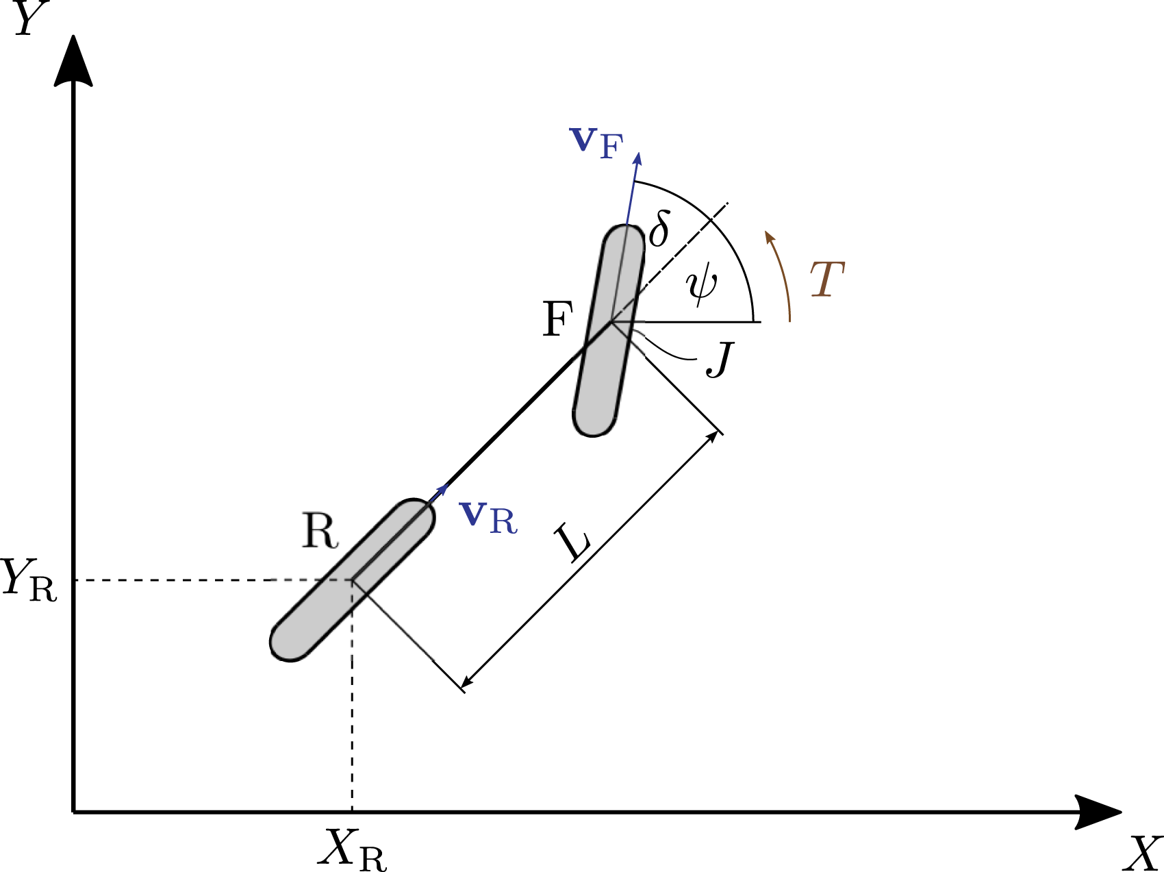

We choose the position coordinates of the rear axle, the yaw angle of the vehicle, and the steering angle as generalized coordinates, leading to the generalized coordinate vector

$\mathbf{q}={\left[\begin{array}{cccc}{X}_{\mathrm{R}}& Y_{\mathrm{R}}& \psi & \delta \end{array}\right]}^{⊺}.$

(1)

Choosing the rear wheel coordinates is a quite standard technique. The resulting equation of motion will have the simplest form in this way. Since no tire deformation is considered in our model (i.e., no side slip occurs), the direction of the velocity vectors at the front and rear axles are at all times determined by the rolling direction of the wheels. This means that the velocity vector v_R at the rear axle is always parallel to the longitudinal axis of symmetry of the vehicle, while the velocity vector v_F at the front wheels always points into the direction defined by the steering angle. Based on the above considerations, the following two kinematic constraints can be formulated

$\begin{array}{l}{\dot{X}}_{\mathrm{R}}\sin \left(\psi +\delta \right)-{\dot{Y}}_{\mathrm{R}}\cos \left(\psi +\delta \right)-L\dot{\psi }\cos \delta =0,\\ -{\dot{X}}_{\mathrm{R}}\sin \psi +{\dot{Y}}_{\mathrm{R}}\cos \psi =0.\end{array}$

(2)

Furthermore, we assume that the longitudinal speed of the vehicle is constant (|v_R|≡ v, corresponding to a rear wheel drive vehicle), which leads to the additional kinematic constraint

${\dot{X}}_{\mathrm{R}}\cos \psi +{\dot{Y}}_{\mathrm{R}}\sin \psi =v.$

(3)

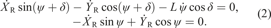
The presence of kinematic constraints makes the vehicle model nonholonomic. To derive the equations of motion of the system, we use the Gibbs–Appell method (Gantmacher (1975)), which requires the definition of so-called pseudo-velocities. Since the number of generalized coordinates is four and the system includes three kinematic constraints, one pseudo-velocity needs to be defined, which we choose to be the steering rate

${\sigma }_1=\dot{\delta }.$

(4)

The three kinematic constraints in (2) and (3) as well as the definition of the pseudo-velocity σ₁ in (4) can be solved for the time derivatives of the generalized coordinates

${\dot{X}}_{\mathrm{R}}=v\cos \psi ,{\dot{Y}}_{\mathrm{R}}=v\sin \psi ,\dot{\psi }=\frac{v}{L}\tan \delta ,\dot{\delta }={\sigma }_1.$

(5)

In addition, the Gibbs–Appell equation leads to the fifth equation of motion, which describes the steering dynamics

${\dot{\sigma }}_1=\frac{T}{J}.$

(6)

3. Hierarchical steering control

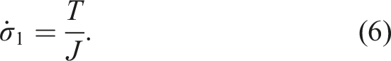
In this section, a hierarchical steering controller is introduced (see Figure 2), taking into account communication and sampling delays. The goal of the controller is to ensure that the vehicle follows a reference path, which is achieved by feeding back the lateral position of the rear axle Y_R and the yaw angle ψ. 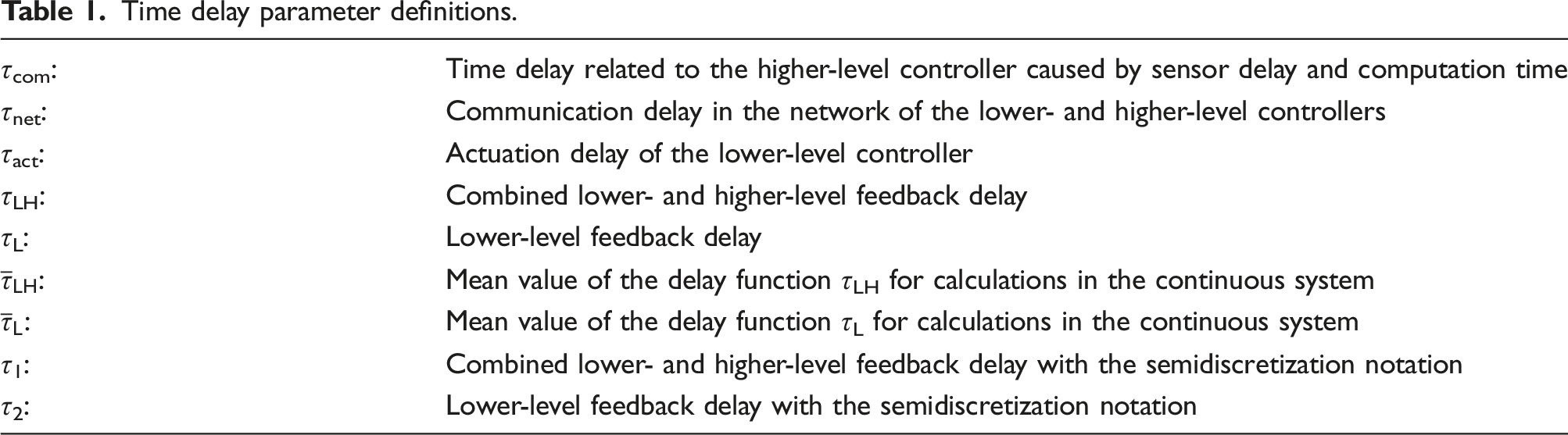Assuming a straight-line reference path along the X axis (Y_R ≡ 0, ψ ≡ 0), the higher-level controller generates the desired steering angle using the proportional gains k _Y and k _ψ as follows

${\stackrel{\sim }{\delta }}_{\mathrm{d}}\left(t\right)=-k_Y{Y}_{\mathrm{R}}\left(t-{\tau }_{\text{com}}\right)-k_{\psi }\psi \left(t-{\tau }_{\text{com}}\right).$

(7)

The time delay τ_com includes the sensor delays, sampling, and computation times. The subscript com refers to computation. The desired steering angle ${\stackrel{\sim }{\delta }}_{\mathrm{d}}$ is then sent to the steering servo with the network delay τ_net that is related to the communication between the two controllers. This means that the reference signal of the lower-level controller is ${\delta }_{\mathrm{d}}\left(t\right)={\stackrel{\sim }{\delta }}_{\mathrm{d}}\left(t-{\tau }_{\text{net}}\right)$ . This controller calculates the steering torque T that is required so that the actual steering angle δ follows the reference value δ_d. This is achieved using the proportional-derivative control law

$\begin{array}{c}T\left(t\right)=-P\left(\delta \left(t-{\tau }_{\text{act}}\right)-{\delta }_{\mathrm{d}}\left(t-{\tau }_{\text{act}}\right)\right)-D\dot{\delta }\left(t-{\tau }_{\text{act}}\right),\end{array}$

(8)

where P and D denote the lower-level control gains, while the actual and desired steering angles δ and δ_d are sampled with the time delay τ_act, where the subscript act refers to actuation. The summary of the delay parameters can be found in Table 1. For the sake of simplicity, the reference steering rate in (8) is set to zero.

Figure 2.

Block diagram of the hierarchical control scheme used for the lateral control of the vehicle.

Table 1.

Time delay parameter definitions.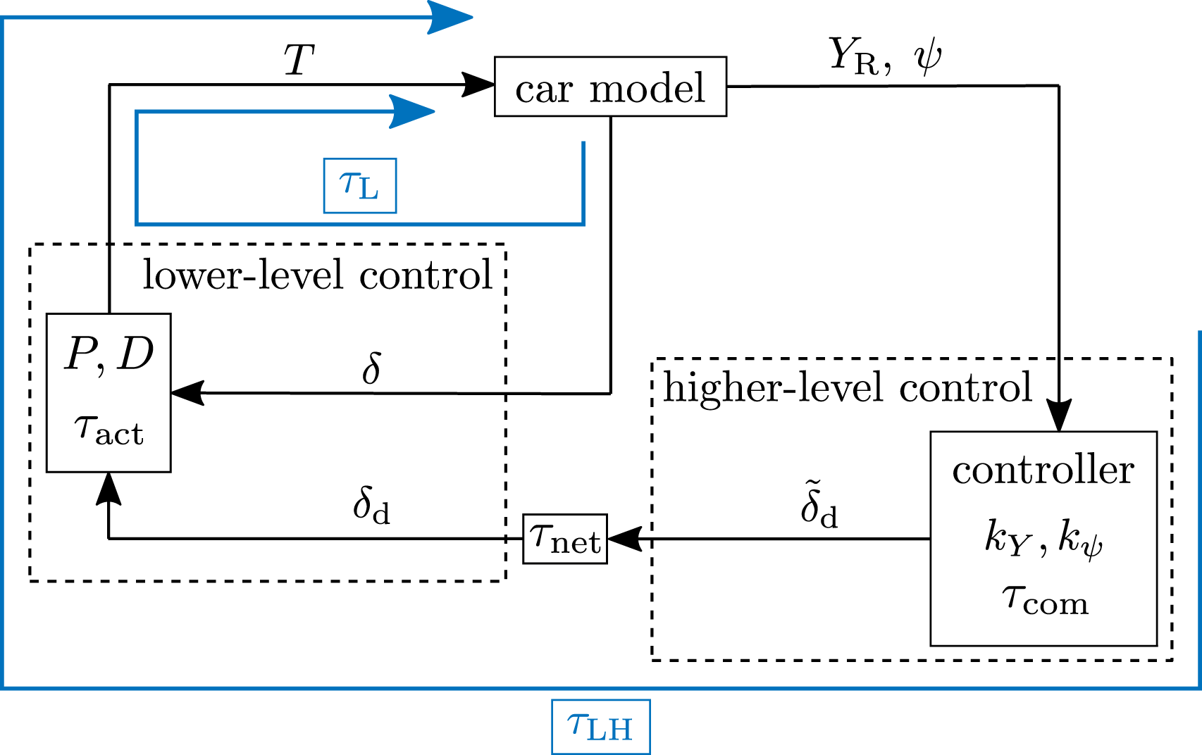

τcom:	Time delay related to the higher-level controller caused by sensor delay and computation time
τnet:	Communication delay in the network of the lower- and higher-level controllers
τact:	Actuation delay of the lower-level controller
τLH:	Combined lower- and higher-level feedback delay
τL:	Lower-level feedback delay
${\overline{\tau }}_{\text{LH}}$ :	Mean value of the delay function τLH for calculations in the continuous system
${\overline{\tau }}_{\mathrm{L}}$ :	Mean value of the delay function τL for calculations in the continuous system
τ1:	Combined lower- and higher-level feedback delay with the semidiscretization notation
τ2:	Lower-level feedback delay with the semidiscretization notation

The control gains P and D can be normalized with respect to the moment of inertia J, leading to the reduced control parameters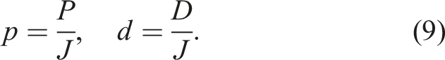

$p=\frac{P}{J},\hspace{1em}d=\frac{D}{J}.$

(9)

Furthermore, we introduce the time delay values related to the control loop as (see Figure 2)

${\tau }_{\mathrm{L}}={\tau }_{\text{act}},{\tau }_{\text{LH}}={\tau }_{\text{com}}+{\tau }_{\text{net}}+{\tau }_{\text{act}}.$

(10)

Therefore, in the closed-loop system, when the hierarchical steering controller is enabled, the dynamics of σ₁ in (6) can be modified to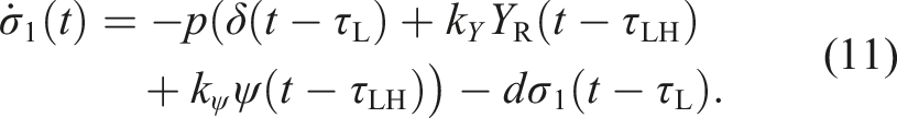

$\begin{array}{c}{\dot{\sigma }}_1\left(t\right)=-p(\delta \left(t-{\tau }_{\mathrm{L}}\right)+k_Y{Y}_{\mathrm{R}}\left(t-{\tau }_{\text{LH}}\right)+k_{\psi }\psi \left(t-{\tau }_{\text{LH}}\right))-d{\sigma }_1\left(t-{\tau }_{\mathrm{L}}\right).\end{array}$

(11)

4. Semidiscretization method for digital controllers with multiple delays

The lane-keeping controller in Section 3 was presented in continuous time, but when implemented in practice, a digital controller will have to be used. This means that due to the effects of digital sampling, the time delays will not remain constant, but they will be continually changing according to time periodic sawtooth-like functions (see Figure 3). A powerful method for performing the linear stability analysis of such digital systems with time periodic time delays is the semidiscretization method (Insperger (2011)). First, we present a brief review of the general concept of semidiscretization for time delay systems, and then we show how it can be extended for the case of multiple discrete delays.

Figure 3.

Illustration of the sawtooth-like time periodic nature of time delays in digital systems.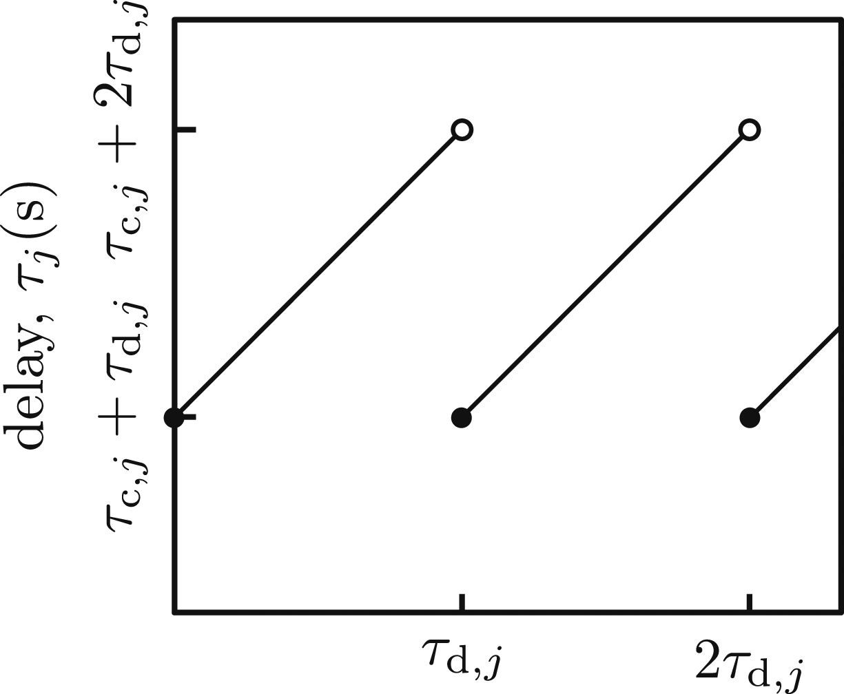

4.1. General concept of semidiscretization

Consider the linear system with multiple continuous point delays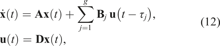

$\begin{array}{l}\stackrel{.}{\mathbf{x}}\left(t\right)=\mathbf{A}\mathbf{x}\left(t\right)+{\displaystyle \sum }_{j=1}^g{\mathbf{B}}_j\mathbf{u}\left(t-{\tau }_j\right),\\ \mathbf{u}\left(t\right)=\mathbf{D}\mathbf{x}\left(t\right),\end{array}$

(12)

where $\mathbf{x}\in {\mathbb{R}}^n$ is the state vector, $\mathbf{u}\in {\mathbb{R}}^m$ is the input, A, B _j , and D are appropriately sized constant matrices, and τ _j are constant point delays. Note that systems with distributed delays as well as time-dependent parameters can also be approximated in the above form (see Insperger (2011) for details).

By introducing the discrete time scale t _i = ih, where $i\in \mathbb{Z}$ and h is the discretization step, the semidiscretization method approximates the delayed terms as constant in each discretization interval [t _i , t_i+1)

$\mathbf{u}\left(t-{\tau }_j\right)\approx \mathbf{u}\left(t_{i-r_j}\right)=\mathbf{u}\left(\left(i-r_j\right)h\right),$

(13)

where r _j = int(τ _j /h) and int denotes the integer-part function. The resulting system can be considered as a set of ordinary differential equations with piecewise constant forcing. Using the variation of constants formula, the solution of the semidiscrete system over one discretization step can be formulated as

${\mathbf{x}}_{i+1}=\mathbf{P}{\mathbf{x}}_i+{\displaystyle \sum }_{j=1}^g{\mathbf{R}}_j{\mathbf{u}}_{i-r_j},$

(14)

where x _i = x(t _i ), u _i = u(t _i ) and

$\mathbf{P}={\mathrm{e}}^{\mathbf{A}h},{\mathbf{R}}_j={\mathbf{B}}_j{\int }_0^h{\mathrm{e}}^{\mathbf{A}\left(h-s\right)}\mathrm{d}s.$

(15)

With the introduction of the augmented state vector

${\mathbf{z}}_i={\left[\begin{array}{ccc}{\mathbf{x}}_i& {\mathbf{u}}_{i-1}& {\mathbf{u}}_{i-2}\dots {\mathbf{u}}_{i-r}\end{array}\right]}^{⊺},$

(16)

where r = max(r _j ), the solution of the system can be formulated as the discrete map

${\mathbf{z}}_{i+1}=\mathbf{G}{\mathbf{z}}_i,$

(17)

with the (n+rm) × (n+rm) coefficient matrix

$\begin{array}{c}\mathbf{G}=\left[\begin{array}{ccccc}\mathbf{P}& \mathbf{0}& \dots & \mathbf{0}& \mathbf{0}\\ \mathbf{D}& \mathbf{0}& \dots & \mathbf{0}& \mathbf{0}\\ \mathbf{0}& \mathbf{I}& \dots & \mathbf{0}& \mathbf{0}\\ ⋮& & \ddots & ⋮& ⋮\\ \mathbf{0}& \mathbf{0}& \dots & \mathbf{I}& \mathbf{0}\end{array}\right]+{\displaystyle \sum }_{j=1}^g\begin{array}{cccc}1& r_j& r& \left[\begin{array}{ccccccc}\mathbf{0}& \mathbf{0}& \dots & {\mathbf{R}}_j& \mathbf{0}& \dots & \mathbf{0}\\ \mathbf{0}& \mathbf{0}& \dots & \mathbf{0}& \mathbf{0}& \dots & \mathbf{0}\\ \mathbf{0}& \mathbf{0}& \dots & \mathbf{0}& \mathbf{0}& \dots & \mathbf{0}\\ ⋮& ⋮& \ddots & ⋮& ⋮& \ddots & ⋮\\ \mathbf{0}& \mathbf{0}& \dots & \mathbf{0}& \mathbf{0}& \dots & \mathbf{0}\end{array}\right].\end{array}\end{array}$

(18)

G can be considered as a finite dimensional matrix representation of the infinite dimensional monodromy operator of the original time delay system in (12), which can be used to assess stability. If all eigenvalues of G are inside the unit circle of the complex plane, the trivial solution z = 0 of the original system is asymptotically stable.

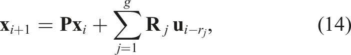
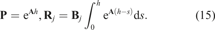
The constant approximation of the delayed terms in (13) corresponds to the sawtooth-like periodic approximation of the constant time delays, as in Figure 3. Therefore, if there is only one delay in the system (g = 1) and the discretization time is set to be equal to the sampling time (r = 1), the semidiscrete system can be used as a model for digital sampling with zero-order hold (Åström and Wittenmark (2011); Ogata (1995); Stépán (2001)). This is, however, more complicated when there are multiple delays present in the system, as in, for example, the hierarchical controller presented in Section 3. Therefore, in the following, we present an extension of the semidiscretization method in order to handle digital controllers with multiple delays. The proposed method will then be used in Section 5 to perform the stability analysis of the closed-loop vehicle model with the hierarchical lane-keeping controller.

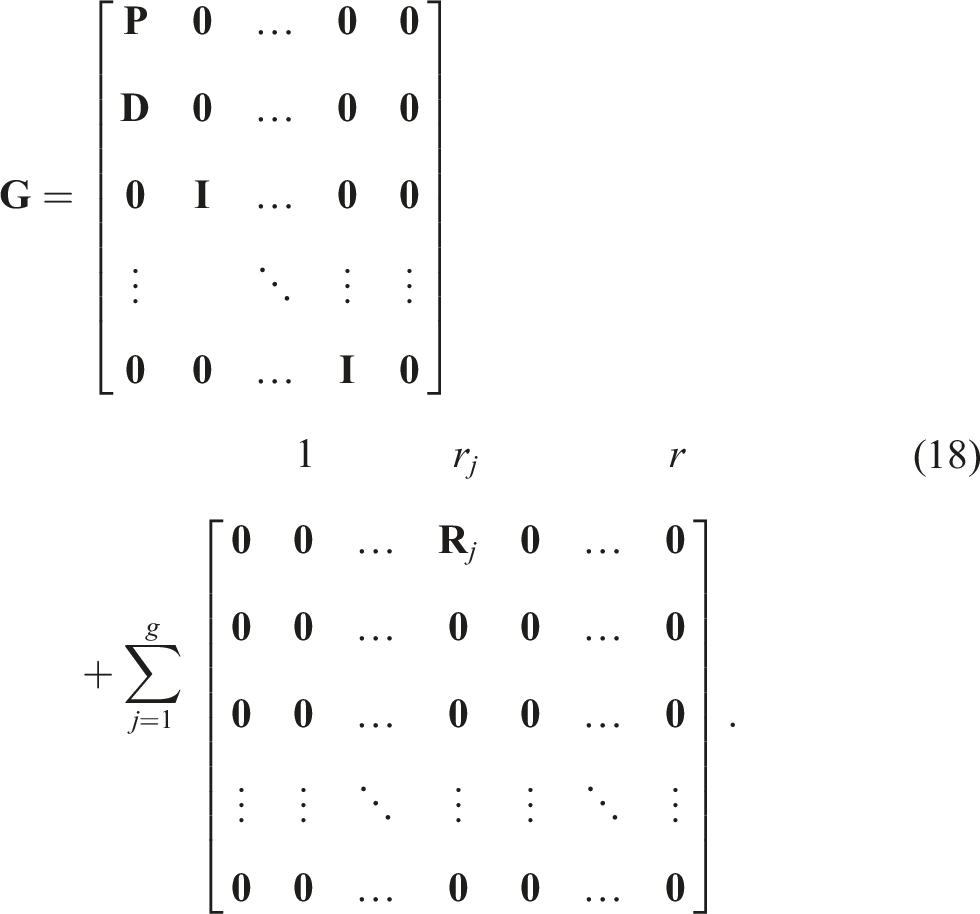
4.2. Extension for systems with multiple discrete time delays

If there are multiple discrete delays in a digital system, each time delay can be characterized by a separate periodic sawtooth-like function. For the jth time delay τ _j , the minimum and maximum of this periodic function is defined as τ_j,s = τ_c,j + τ_d,j and τ_j,e = τ_c,j + 2τ_d,j, respectively, as in Figure 3. The subscripts c and d refer to the continuous and digital parts of the delay functions, respectively; furthermore, subscripts s and e mean the starting value and end value of the sawtooth-like time periodic functions. The time period of the τ _j (t) function will then be τ_e,j−τ_s,j. The following integers can be introduced to denote the rounded length of τ_s,j and τ_e,j in terms of multiples of the discretization step h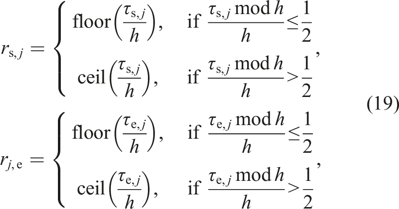

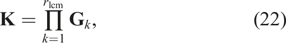
$\begin{array}{c}{r}_{\mathrm{s},j}=\{\begin{array}{cc}\text{floor}\left(\frac{{\tau }_{\mathrm{s},j}}{h}\right),& \text{if}\frac{{\tau }_{\mathrm{s},j}\mathrm{mod}\hspace{0.17em}h}{h}\le \frac{1}{2}\\ \text{ceil}\left(\frac{{\tau }_{\mathrm{s},j}}{h}\right),& \text{if}\frac{{\tau }_{\mathrm{s},j}\mathrm{mod}\hspace{0.17em}h}{h}>\frac{1}{2}\end{array},\\ r_{j,\mathrm{e}}=\{\begin{array}{cc}\text{floor}\left(\frac{{\tau }_{\mathrm{e},j}}{h}\right),& \text{if}\frac{{\tau }_{\mathrm{e},j}\mathrm{mod}\hspace{0.17em}h}{h}\le \frac{1}{2}\\ \text{ceil}\left(\frac{{\tau }_{\mathrm{e},j}}{h}\right),& \text{if}\frac{{\tau }_{\mathrm{e},j}\mathrm{mod}\hspace{0.17em}h}{h}>\frac{1}{2}\end{array},\end{array}$

(19)

where mod is the modulo function. Furthermore, we define the difference of these values

$r_{\text{step},j}=r_{\mathrm{e},j}-r_{\mathrm{s},j},$

(20)

which gives the rounded time period of the periodic delay function in terms of h. A full period of the whole system (the principal period) is only completed when all the individual periodic τ _j (t) functions are at the end of their time period. Therefore, the length of the principal period r_lcm in terms of discretization steps can be calculated as the least common multiple (lcm) of the individual time periods r_step,j

$r_{\text{lcm}}=\text{lcm}\left(r_{\text{step},j}\right)-1.$

(21)

In order to assess the stability of the system, the matrix representation of the monodromy operator must be determined as the solution matrix of the semidiscrete system over the principal period. This involves r_lcm discretization periods; therefore, if the solution matrix over one discretization step is denoted by G, then the monodromy operator can be approximated by the geometric series

$\mathbf{K}={\displaystyle \prod }_{k=1}^{r_{\text{lcm}}}{\mathbf{G}}_k,$

(22)

and the monodromy mapping over one principal period will be

${\mathbf{z}}_{i+1}=\mathbf{K}{\mathbf{z}}_i.$

(23)

In order to account for the sawtooth-like periodicity of each individual time delay, the positions of 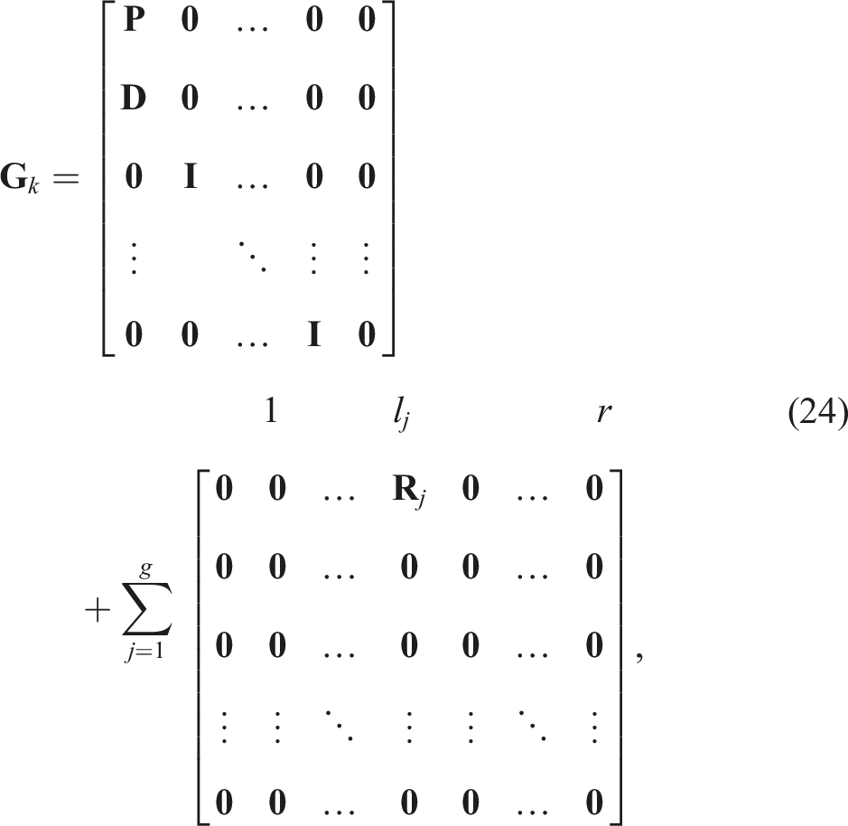R _j will be shifting in the matrices G _k , that is, each G _k will be different

$\begin{array}{c}{\mathbf{G}}_k=\left[\begin{array}{ccccc}\mathbf{P}& \mathbf{0}& \dots & \mathbf{0}& \mathbf{0}\\ \mathbf{D}& \mathbf{0}& \dots & \mathbf{0}& \mathbf{0}\\ \mathbf{0}& \mathbf{I}& \dots & \mathbf{0}& \mathbf{0}\\ ⋮& & \ddots & ⋮& ⋮\\ \mathbf{0}& \mathbf{0}& \dots & \mathbf{I}& \mathbf{0}\end{array}\right]+{\displaystyle \sum }_{j=1}^g\begin{array}{cccc}1& l_j& r& \left[\begin{array}{ccccccc}\mathbf{0}& \mathbf{0}& \dots & {\mathbf{R}}_j& \mathbf{0}& \dots & \mathbf{0}\\ \mathbf{0}& \mathbf{0}& \dots & \mathbf{0}& \mathbf{0}& \dots & \mathbf{0}\\ \mathbf{0}& \mathbf{0}& \dots & \mathbf{0}& \mathbf{0}& \dots & \mathbf{0}\\ ⋮& ⋮& \ddots & ⋮& ⋮& \ddots & ⋮\\ \mathbf{0}& \mathbf{0}& \dots & \mathbf{0}& \mathbf{0}& \dots & \mathbf{0}\end{array}\right],\end{array}\end{array}$

(24)

where the location of the jthcoefficient matrix R _j in the upper right block of G _k will be shifting in each iteration according to

$l_j=r_{\mathrm{s},j}+k\mathrm{mod}\hspace{0.17em}{r}_{\text{step},j}$

(25)

and

$r=\max \left(r_{\mathrm{e},j}\right)-1.$

(26)

In the first iteration (k = 0), the position of the matrices R _j will be r_s,j, corresponding to the minimum of each sawtooth function. As the iteration continues, the position of every R _j will increase until the corresponding maximum r_e,j (representing the peak of the jth sawtooth function), after which it jumps back to its initial position r_s,j. A complete period is reached (k = r_lcm−1) once all the coefficient matrices reach their end positions r_e,j at the same time. This requires that all r_s,j and r_e,j values are multiples of the discretization step h, which is ensured by the floor and ceiling functions in (19). With the multiplication of the individual G _k matrices, the matrix of the discrete mapping K can be calculated. If all the eigenvalues of K are inside the unit circle of the complex plane, the system with multiple discrete time delays is asymptotically stable.

Note that while the constant approximation of the delayed terms over the discretization step h inherently introduces a sawtooth-like periodicity of length h in each time delay, the shifting position of the coefficient matrices R _j in (24) ensures that the longer time period of discrete delays that are larger than h can also be considered.

5. Stability analysis

In this section, we perform the linear stability analysis of the vehicle model with the hierarchical lane-keeping controller as defined in (5) and (11), for the steady state of rectilinear motion along the X axis. This corresponds to the state variables

$X_{\mathrm{R}}=vt,Y_{\mathrm{R}}\equiv 0,\psi \equiv 0,\delta \equiv 0,{\sigma }_1\equiv 0.$

(27)

Since the lane-keeping controller in Section 3 is based on only the lateral position Y_R and the yaw angle ψ, the equation of X_R can be decoupled from the rest, leading to the reduced state vector

$\mathbf{x}={\left[\begin{array}{cccc}{Y}_{\mathrm{R}}& \psi & \delta & {\sigma }_1\end{array}\right]}^{⊺}.$

(28)

Linearizing the remaining equations of the closed-loop system around (27) leads to the system of linear differential equations

$\stackrel{.}{\mathbf{x}}\left(t\right)=\mathbf{A}\mathbf{x}\left(t\right)+{\mathbf{B}}_{\mathrm{L}}\mathbf{x}\left(t-{\tau }_{\mathrm{L}}\right)+{\mathbf{B}}_{\text{LH}}\mathbf{x}\left(t-{\tau }_{\text{LH}}\right),$

(29)

where

$\begin{array}{l}\mathbf{A}=\left[\begin{array}{cccc}0& v& 0& 0\\ 0& 0& \frac{v}{L}& 0\\ 0& 0& 0& 1\\ 0& 0& 0& 0\end{array}\right],{\mathbf{B}}_{\mathrm{L}}=\left[\begin{array}{cccc}0& 0& 0& 0\\ 0& 0& 0& 0\\ 0& 0& 0& 0\\ 0& 0& -p& -d\end{array}\right],\\ {\mathbf{B}}_{\text{LH}}=\left[\begin{array}{cccc}0& 0& 0& 0\\ 0& 0& 0& 0\\ 0& 0& 0& 0\\ -p{k}_Y& -p{k}_{\psi }& 0& 0\end{array}\right].\end{array}$

(30)

In the following, we perform the stability analysis of the system in order to uncover the regions of control gains that can stabilize the straight-line motion of the vehicle. The derivations will be performed for both the continuous and the discrete time control case so that the difference in results between the two modeling approaches can be highlighted.

5.1. Continuous case

The stability boundaries for continuous time delays can be calculated using the D-subdivision method (Insperger (2011)). In the continuous case, let us represent the periodically changing digital time delays with their means, which will be denoted by overbars, that is, ${\overline{\tau }}_{\mathrm{L}}$ and ${\overline{\tau }}_{\text{LH}}$ will be constant, continuous time delays. The linearized system in this case can be written as

$\stackrel{.}{\mathbf{x}}\left(t\right)=\mathbf{A}\mathbf{x}\left(t\right)+{\mathbf{B}}_{\mathrm{L}}\mathbf{x}\left(t-{\overline{\tau }}_{\mathrm{L}}\right)+{\mathbf{B}}_{\text{LH}}\mathbf{x}\left(t-{\overline{\tau }}_{\text{LH}}\right),$

(31)

which leads to the characteristic equation

$D\left(\lambda \right):=\det \left(\mathbf{A}+{\mathbf{B}}_{\mathrm{L}}{\mathrm{e}}^{-\lambda {\overline{\tau }}_{\mathrm{L}}}+{\mathbf{B}}_{\text{LH}}{\mathrm{e}}^{-\lambda {\overline{\tau }}_{\text{LH}}}\right)=0,$

(32)

where $\lambda \in \mathbb{C}$ is the characteristic exponent. Evaluating the determinant in (32) results in

$\begin{array}{c}{\lambda }^4+{\lambda }^{3}d{\mathrm{e}}^{-\lambda {\overline{\tau }}_{\mathrm{L}}}+{\lambda }^{2}p{\mathrm{e}}^{-\lambda {\overline{\tau }}_{\mathrm{L}}}+\lambda \frac{p{k}_{\psi }v}{L}{\mathrm{e}}^{-\lambda {\overline{\tau }}_{\text{LH}}}+\frac{p{k}_Y{v}^2}{L}{\mathrm{e}}^{-\lambda {\overline{\tau }}_{\text{LH}}}=0.\end{array}$

(33)

If the characteristic exponent is zero, that is, λ = 0, static loss of stability will occur. This happens if

$\frac{p{k}_Y{v}^2}{L}=0,$

(34)

namely, the vehicle will lose its stability without oscillations at the control gain values p = 0 and k _Y = 0. In addition, oscillatory stability loss can happen if a complex conjugate pair of characteristic roots crosses the imaginary axis at λ = ±iω. Substituting λ = iω into the characteristic equation in (33) and separating the real and imaginary parts of the resulting equation, the boundaries of dynamic stability loss can be expressed in terms of two arbitrary system parameters, as a parametric function of the oscillation frequency ω.

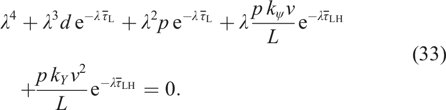
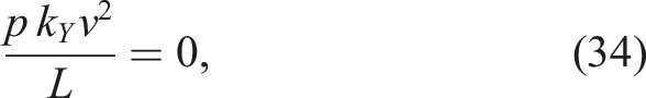
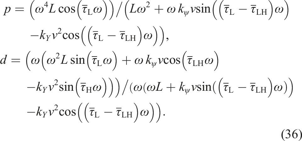
Considering the control gains of the higher-level controller, the stability boundaries are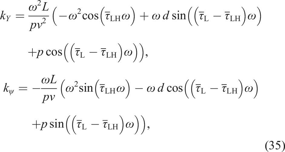

$\begin{array}{l}{k}_Y=\frac{{\omega }^{2}L}{p{v}^2}\left(-{\omega }^2\cos \left({\overline{\tau }}_{\text{LH}}\omega \right)+\omega d\sin \left(\left({\overline{\tau }}_{\mathrm{L}}-{\overline{\tau }}_{\text{LH}}\right)\omega \right)+p\cos \left(\left({\overline{\tau }}_{\mathrm{L}}-{\overline{\tau }}_{\text{LH}}\right)\omega \right)\right),\\ k_{\psi }=-\frac{\omega L}{pv}\left({\omega }^2\sin \left({\overline{\tau }}_{\text{LH}}\omega \right)-\omega d\cos \left(\left({\overline{\tau }}_{\mathrm{L}}-{\overline{\tau }}_{\text{LH}}\right)\omega \right)+p\sin \left(\left({\overline{\tau }}_{\mathrm{L}}-{\overline{\tau }}_{\text{LH}}\right)\omega \right)\right),\end{array}$

(35)

while in terms of the lower-level control gains, stability loss occurs at

$\begin{array}{l}p=\left({\omega }^{4}L\cos \left({\overline{\tau }}_{\mathrm{L}}\omega \right)\right)/\left(L{\omega }^2+\omega k_{\psi }v\sin \left(\left({\overline{\tau }}_{\mathrm{L}}-{\overline{\tau }}_{\text{LH}}\right)\omega \right)-k_Y{v}^2\cos \left(\left({\overline{\tau }}_{\mathrm{L}}-{\overline{\tau }}_{\text{LH}}\right)\omega \right)\right),\\ d=(\omega ({\omega }^{2}L\sin \left({\overline{\tau }}_{\mathrm{L}}\omega \right)+\omega k_{\psi }v\cos \left({\overline{\tau }}_{\text{LH}}\omega \right)\\ -k_Y{v}^2\sin \left({\overline{\tau }}_{\mathrm{H}}\omega \right)))/(\omega (\omega L+k_{\psi }v\sin (\left({\overline{\tau }}_{\mathrm{L}}-{\overline{\tau }}_{\text{LH}}\right)\omega ))\\ -k_Y{v}^2\cos \left(\left({\overline{\tau }}_{\mathrm{L}}-{\overline{\tau }}_{\text{LH}}\right)\omega \right)).\end{array}$

(36)

5.2. Digital system

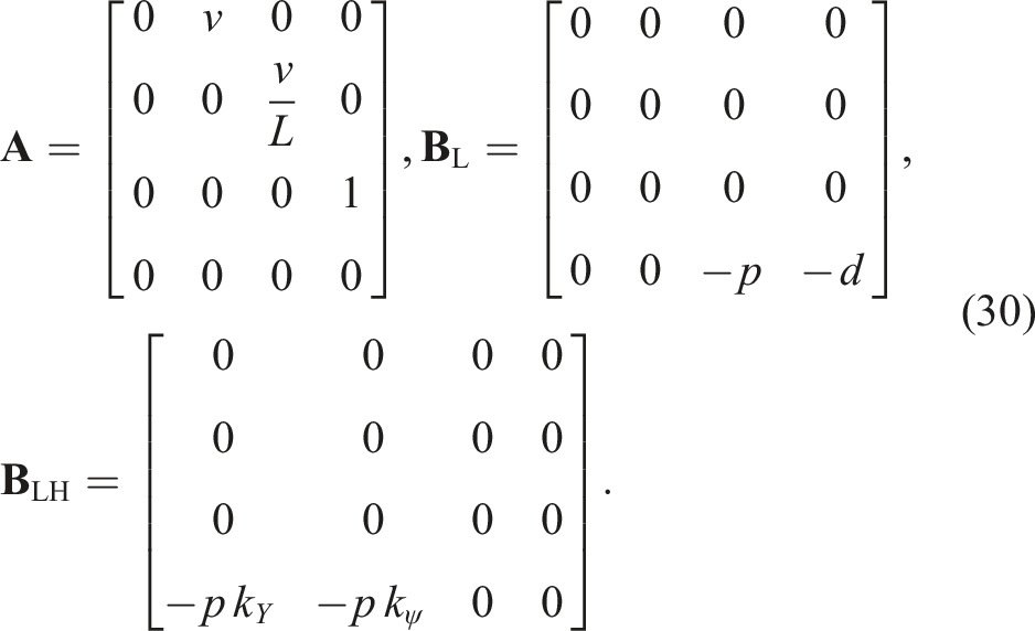
For the stability analysis of the discrete time case, we used the semidiscretization method as detailed in Section 4.2. The linearized system in (29) can be brought to the form in (12) by defining D as the four-dimensional identity matrix, that is, u = x. In the digital case, the value of the time periodic delay τ₂ = τ_L of the lower-level controller ranges from τ_act to 2τ_act, while the combined delay τ₁ = τ_LH of the two controller levels has a minimum of τ_com+τ_net+τ_act and a maximum of τ_com+2τ_net+τ_act, as illustrated in Figure 4. According to Section 4, τ_c,1 = τ_com+τ_act, τ_d,1 = τ_net and τ_c,2 = 0, τ_d,2 = τ_act are the parameters of the combined and the lower-level time delay functions, respectively.

Figure 4.

Sawtooth-like time periodic delay functions of the digital system. The time delay of the lower- and higher-level controller together can be seen in (a) and the lower-level controller in (b).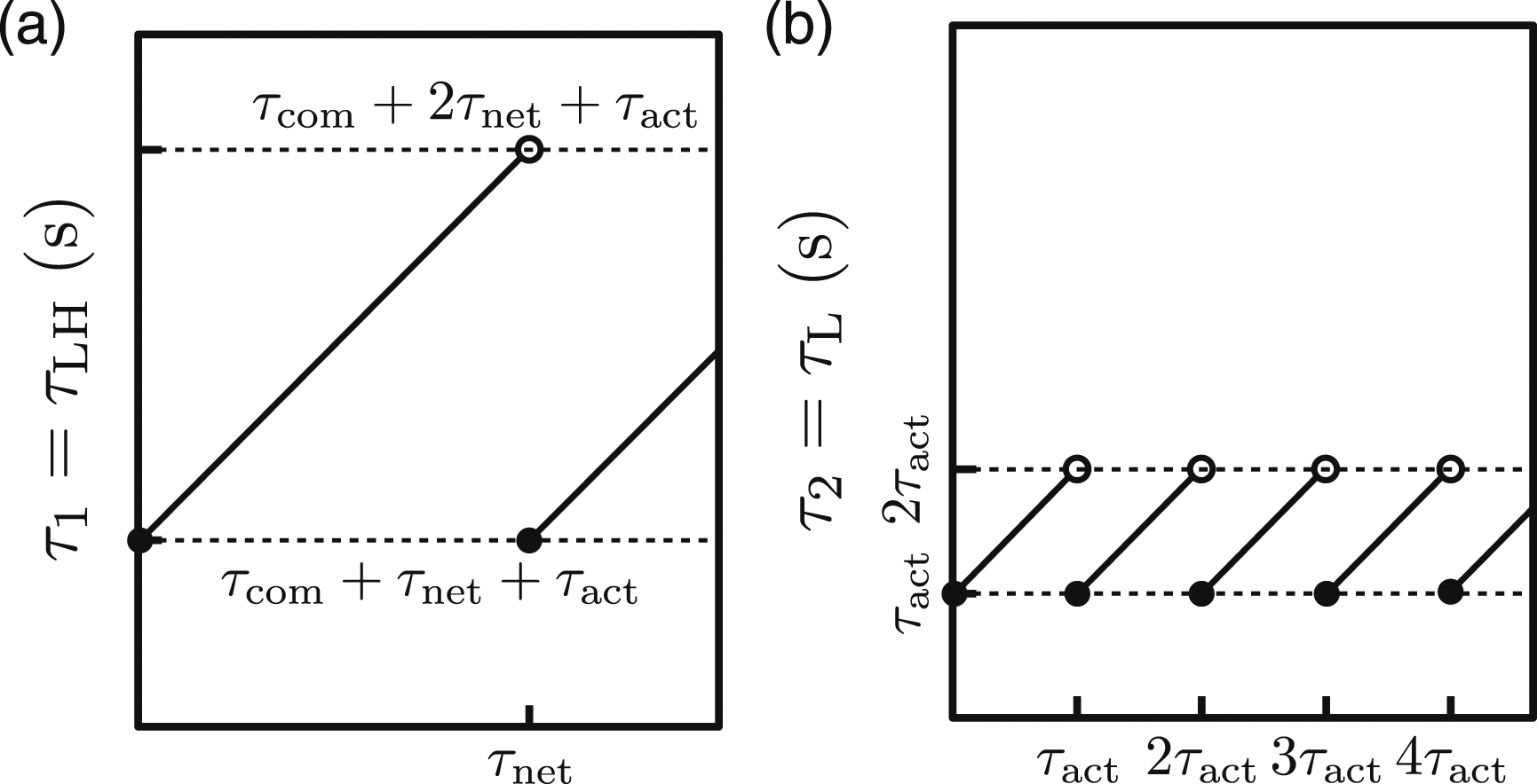

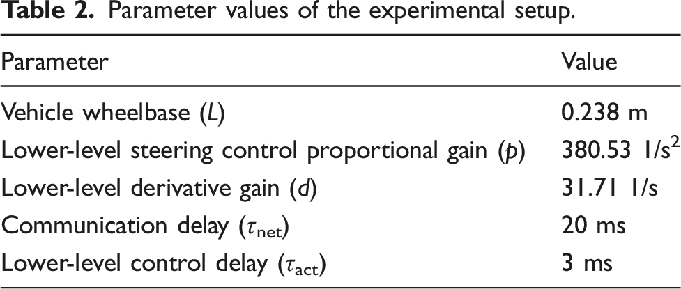
In the experimental setup detailed in Section 6, the higher-level control delay τ_com can be altered programmatically. The sampling frequency between the lower- and higher-level controllers is 50 Hz, corresponding to τ_net = 20 ms, while the sampling frequency of the actuator is 330 Hz, leading to τ_act ≈ 3 ms. With the consideration of these delay values, the discretization time step was chosen to be h = 1 ms during the calculations.

5.3. Comparison

Figure 5(i) shows the stability charts of stabilizing control gains for both the continuous and discrete time delay cases. The stability charts were generated using the parameter values listed in Table 2, corresponding to the experimental setup in Section 6. The delay of the higher-level controller was set to τ_com = 1 ms.

Figure 5.

(i) Comparison of the stability boundaries for the continuous and digital systems. The time delays of the continuous and digital systems are ${\overline{\tau }}_{\mathrm{L}}=4.5\text{ms},{\overline{\tau }}_{\text{LH}}=34\text{ms}$ and τ_com = 1 ms, τ_net = 20 ms, τ_act = 3 ms, respectively. The red markers give the best performance controllers, which coincide for the continuous and digital systems in both parameter planes. (ii) Parameter analysis investigating the sampling time delay τ_com. The other time delays are τ_net = 20 ms, τ_act = 3 ms. The parameters of the best performance points for different sampling time delay τ_com values can be found in Table 3. The parameter planes are (a) k _Y −k _ψ and (b) p−d. The velocity for all the results is v = 10 m/s. The continuous and dashed lines show the results of the digital and continuous systems, respectively.

Table 2.

Parameter values of the experimental setup.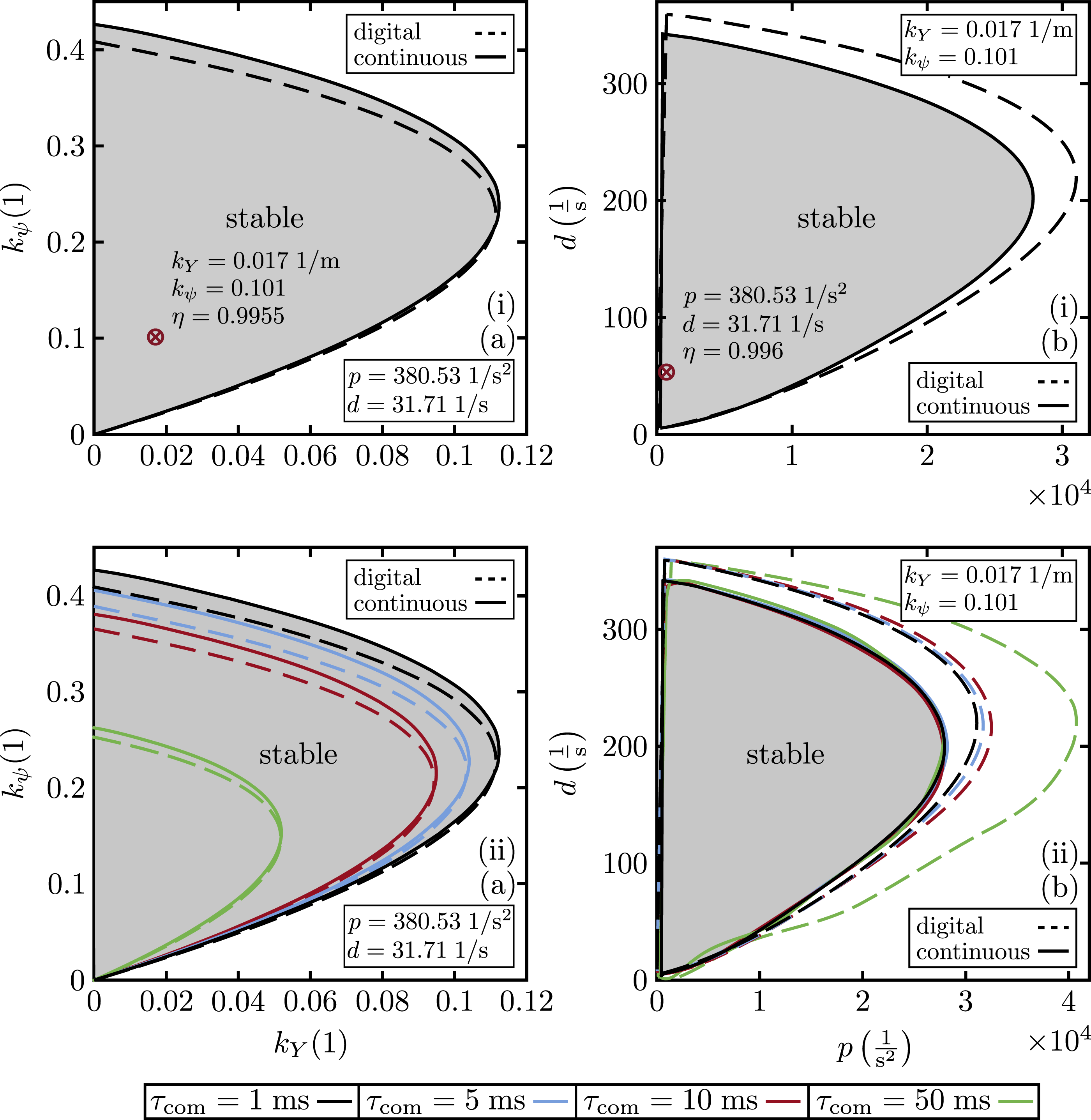

Parameter	Value
Vehicle wheelbase (L)	0.238 m
Lower-level steering control proportional gain (p)	380.53 1/s2
Lower-level derivative gain (d)	31.71 1/s
Communication delay (τnet)	20 ms
Lower-level control delay (τact)	3 ms

The continuous approximation of the discrete delays can be calculated as the mean value of the sawtooth-like functions. This corresponds to ${\overline{\tau }}_{\mathrm{L}}=3/2{\tau }_{\text{act}}$ and ${\overline{\tau }}_{\text{LH}}={\tau }_{\text{com}}+3/2{\tau }_{\text{net}}+{\tau }_{\text{act}}$ (see Figure 4).

Figure 5(i)(a) shows the stable region of the higher-level control gains k _Y and k _ψ .

It can be seen that there is negligible difference in the stability boundaries between the continuous and the digital system. The difference is more pronounced in the plane of the lower-level control gains p and d in Figure 5(i)(b), but the continuous approximation is still reasonably accurate.

In order to find the best performance point of the system, where the most highly damped system response can be achieved, we introduce the maximum normalized eigenvalue of the discrete mapping as

$\eta ={\left|{\mu }_{\max }\right|}^{\frac{1}{r_{\text{lcm}}}},$

(37)

where μ denotes the eigenvalues of the discrete mapping. The normalization is necessary only when the periods of the delay functions change in the investigated stability region. The global optima in Figure 5(i) are denoted by red dots. These points coincide for the continuous and digital systems. The parameters of the best performance points from Figure 5(i) can be found in Table 3.

Table 3.

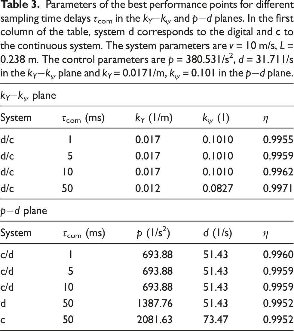
Parameters of the best performance points for different sampling time delays τ_com in the k _Y −k _ψ and p−d planes. In the first column of the table, system d corresponds to the digital and c to the continuous system. The system parameters are v = 10 m/s, L = 0.238 m. The control parameters are p = 380.531/s², d = 31.711/s in the k _Y −k _ψ plane and k _Y = 0.0171/m, k _ψ = 0.101 in the p−d plane.

k Y −k ψ plane
System	τcom (ms)	k Y (1/m)	k ψ (1)	η
d/c	1	0.017	0.1010	0.9955
d/c	5	0.017	0.1010	0.9959
d/c	10	0.017	0.1010	0.9962
d/c	50	0.012	0.0827	0.9971

p−d plane
System	τcom (ms)	p (1/s2)	d (1/s)	η
c/d	1	693.88	51.43	0.9960
c/d	5	693.88	51.43	0.9959
c/d	10	693.88	51.43	0.9959
d	50	1387.76	51.43	0.9952
c	50	2081.63	73.47	0.9952

Based on these results, it is advisable to choose relatively smaller control gains when tuning the higher-level controller (Figure 5(i)(a)). Even though the system would remain linearly stable with larger values of k _Y and k _ψ , the larger gains would not lead to better control performance. In case of the lower-level controller (Figure 5(i)(b)), the optimal gains in terms of system response are very close to the stability boundary, which could easily lead to stability loss due to, for example, modeling uncertainties or control gain perturbations. Therefore, a balance needs to be found between system response and robustness against undesirable effects when tuning the lower-level controller.

Figure 5(ii) shows the effect of increasing the higher-level control delay τ_com on the stable domains. Larger delay values significantly reduce the stable region in the plane of the higher-level control gains k _Y and k _ψ (see Figure 5(ii)(a)), while there is negligible difference between the stability boundaries of the continuous and the digital system. The stable region of the lower-level control gains p and d (Figure 5(ii)(b)) is not affected as much by the value of τ_com, but the difference between the stability boundaries of the continuous and the digital system is becoming more pronounced as τ_com is increased. In the case of τ_com = 50 ms, neglecting the effects of quantization can lead to a significant overestimation of the stable domain. This implies that taking into account the quantized nature of the digital system is more important when tuning the lower-level controller, especially in the case of larger time delays.

6. Measurement results

A series of measurements was carried out using the experimental test rig shown in Figure 6 (see Vörös et al. (2021) for more details). The measurement setup consists of a small-scale model vehicle and a conveyor belt. The vehicle is anchored to the frame of the conveyor belt using a custom suspension mechanism that only constrains the displacement of the car in the longitudinal direction of the belt, while leaving the rest of the degrees of freedom free. The suspension system includes a roller bearing linear guide with a linear encoder, as well as a 3D printed mechanism with ball bearings and magnetic rotary sensors. The running conveyor belt provides the longitudinal velocity of the vehicle, while the steering torque is generated by a servo motor using the controller in (8). The sensor setup provides measurements of the lateral position and yaw angle of the vehicle, and a National Instruments (NI) CompactRIO 9039 unit is used for data acquisition and processing. The higher-level controller in (7) is also running on the NI control unit, where the control gains k _Y −k _ψ and the sampling delay τ_com can be adjusted programmatically. The values of the lower-level control gains and the delays τ_net and τ_act are fixed, as listed in Table 2.

Figure 6.

Measurement setup for the validation process. It consists of a conveyor belt, a linear guide, and the small-scale model of the car. The conveyor belt can run with constant velocities. The guide constrains the displacement in the longitudinal direction, while leaving the rest of the degrees of freedom of the car free.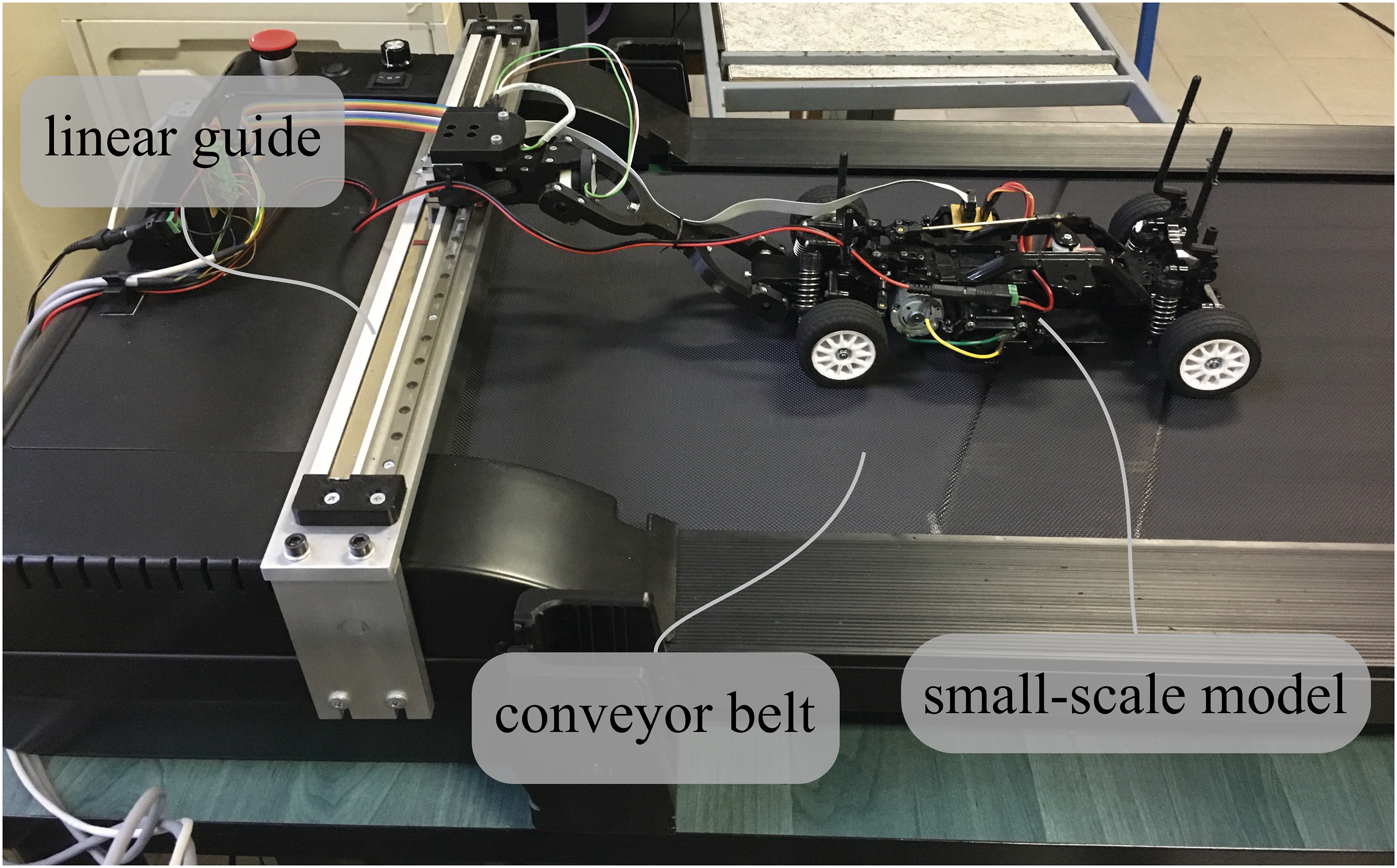

The validating measurements were carried out with velocities v = 1.5 m/s and v = 2.5 m/s, and the stability of the system was assessed for different sets of k _Y –k _ψ values. The measurement points along with the stability boundary of the digital model are plotted in Figure 7. The shape of the experimentally determined stability boundaries show good correspondence with the analytical solution, but there are some large quantitative differences at certain parts of the stability charts. These differences can potentially be explained by the simplifications of our mechanical model: on the one hand, neglecting the tire side forces and side slip angles can have a strong effect on the dynamics of the vehicle. On the other hand, some dissipation effects due to viscous damping and friction might be present in the linear guide, which could also alter the results. Moreover, nonlinear effects not investigated in this study can make it hard to measure the exact stability boundaries. Nevertheless, the analytical results still provide a reasonably accurate prediction of stabilizing control gains. In future studies, the results can be improved, and the system can be investigated more in detail. A more complicated car model can be used with elastic wheels that take the forces and friction into account. Furthermore, the model of the lower-level control scheme can be improved as well.

Figure 7.

Measurement results for velocities (a) v = 1.5 m/s and (b) v = 2.5 m/s in the k _Y −k _ψ plane for τ_com = 1 ms. The rest of the parameters are listed in Table 2. The green circles and red crosses are stable and unstable measured points, respectively. The black line is the analytical result for the digital controller.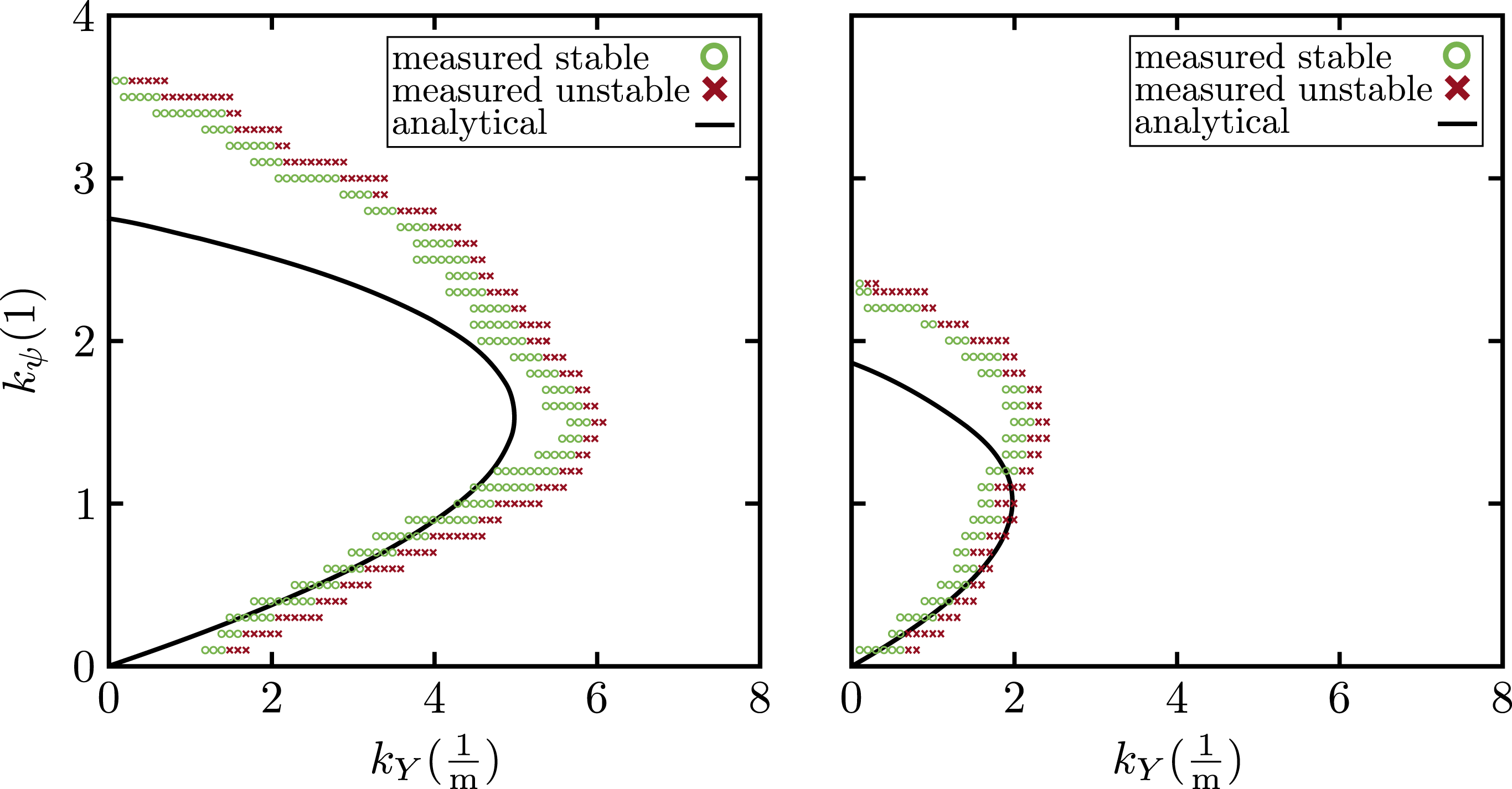

Overall, the measurement results confirm the location and shape of the domain of stabilizing control gains of the higher-level control law. However, since the difference between the analytical results based on the continuous and the digital system model in the plane of the higher-level control gains was negligible (see Figure 5(i)(a) and (ii)(a)), the measurement results provide no additional insight into the effects of digitization, that is, the measurement uncertainties already lead to larger discrepancies in the stability charts than the calculated differences between the continuous and the digital system. Based on Figure 5 (i)(b) and (ii)(b), measurements in the plane of the lower-level control gains could potentially provide a clearer picture regarding the effects of digitization.

7. Conclusion

This study investigated the stability of a lane-keeping controller with hierarchical digital feedback control. The single track kinematic model of cars was used in which the steering dynamics was also considered. The differential equations were derived and the linearization provided the mathematical expressions of the vehicle model. Delayed control laws of a simple lane-keeping controller were implemented.

To construct linear stability charts of the controller, the theory of the semidiscretization method was expanded in a way that digital systems with several delays can be investigated. Using this method together with the D-subdivision method, the stability charts of both continuous and digital systems have been determined highlighting the effects of quantization on the stability of the system.

The results showed that for small higher-level sampling time delays (τ_com), the difference is negligible both in the plane of the lower- and higher-level control gains. However, the parameter analysis implies that for increasing τ_com higher-level sampling time delays, the differences between the continuous and digital systems in the plane of the lower-level control parameter gains p, d are getting more pronounced and non-negligible.

A measurement setup was built with a hierarchical control scheme, which is closely related to the ones used in real, full scale vehicles. Theoretical stability limits of the digital system were compared with the measurement results. The measured and calculated stability properties showed good correspondence. However, based on the calculated stability charts in the plane of the higher-level control gains, the effect of digitization is not severe in this particular system; therefore, the measurement results could not be used to verify the importance of digital effects. The analytical results suggest that experiments in the plane of the lower-level control gains could potentially provide more conclusive results regarding the importance of digitization in the model. Additionally, in other, more detailed models of the controlled vehicle, the effect of digitization might also prove to be more pronounced.

This can be true for other engineering applications as well, especially where the system is described by neutral or advanced delay differential equations (Insperger et al. (2010); Insperger and Kovacs (2017)). Another aspect, which is also an outlook of this study, is that the digital nature of controllers can have significant effects on the nonlinear behavior of dynamical systems (Gyebrószki and Csernák (2019)). Investigating how the digital effects influence the nonlinear behavior of the controlled vehicle is an important direction of future research.