DMVT-based observer design for general affine class of fractional-order nonlinear MIMO systems

Abstract

In this article, a new observer design technique is proposed for the general affine class of fractional-order nonlinear multi-input/multi-output (MIMO) systems. This study is presented based on the differential mean value theorem. One significant characteristic of the suggested approach is that the nonlinear dynamic of observer error is converted into a linear parameter-varying system. Stability and convergence of observation error are shown using the Lyapunov direct method leading to feasibility and existence of a solution for some linear matrix inequalities. The performance and efficacy of the proposed method are evaluated through some illustrated simulations.

1. Introduction

Over the past three centuries, the role of fractional calculus has received increasing attention across several disciplines, and it has been vigorously challenged by many researchers (Dabiri and Butcher, 2019). Recently, its employment in physics and engineering has attracted considerable interest. For example, heat conduction (Jenson and Jeffreys, 1977), transmission line model (Chen and Friedman, 2005), biological and financial systems (Laskin, 2000), dielectric and electrode–electrolyte polarization (Ichise et al., 1971; Sun et al., 1984), and diffusion waves (Ahmad and Sayed, 1996) can be stated for its applications.

Most control systems use state variables of the plants in their control policy. Unfortunately, in practice, it is not possible to access or measure all state variables of an under-control system. Therefore, for implementing such controllers, it is required to estimate unmeasurable states truly. An observer can accomplish this aim. So far, several linear and nonlinear observers have been widely developed by researchers to estimate unmeasurable states of various classes in nonlinear dynamic systems (Chen and Saif, 2012; Dadras and Momeni, 2011; Khalifa and Mabrouk, 2015; Luenberger, 1964). More recent studies on state observers can be found in the literature, such as state feedback control (Gao et al., 2019), fault detection and isolation (Ren-Jie and Jun-Guo, 2022; Su et al., 2016), system monitoring (Anagnostou et al., 2018; Yunlong et al., 2022), observer-based robust adaptive fuzzy control (Ghavidel and Kalat, 2018), and robot manipulator (Yang et al., 2020).

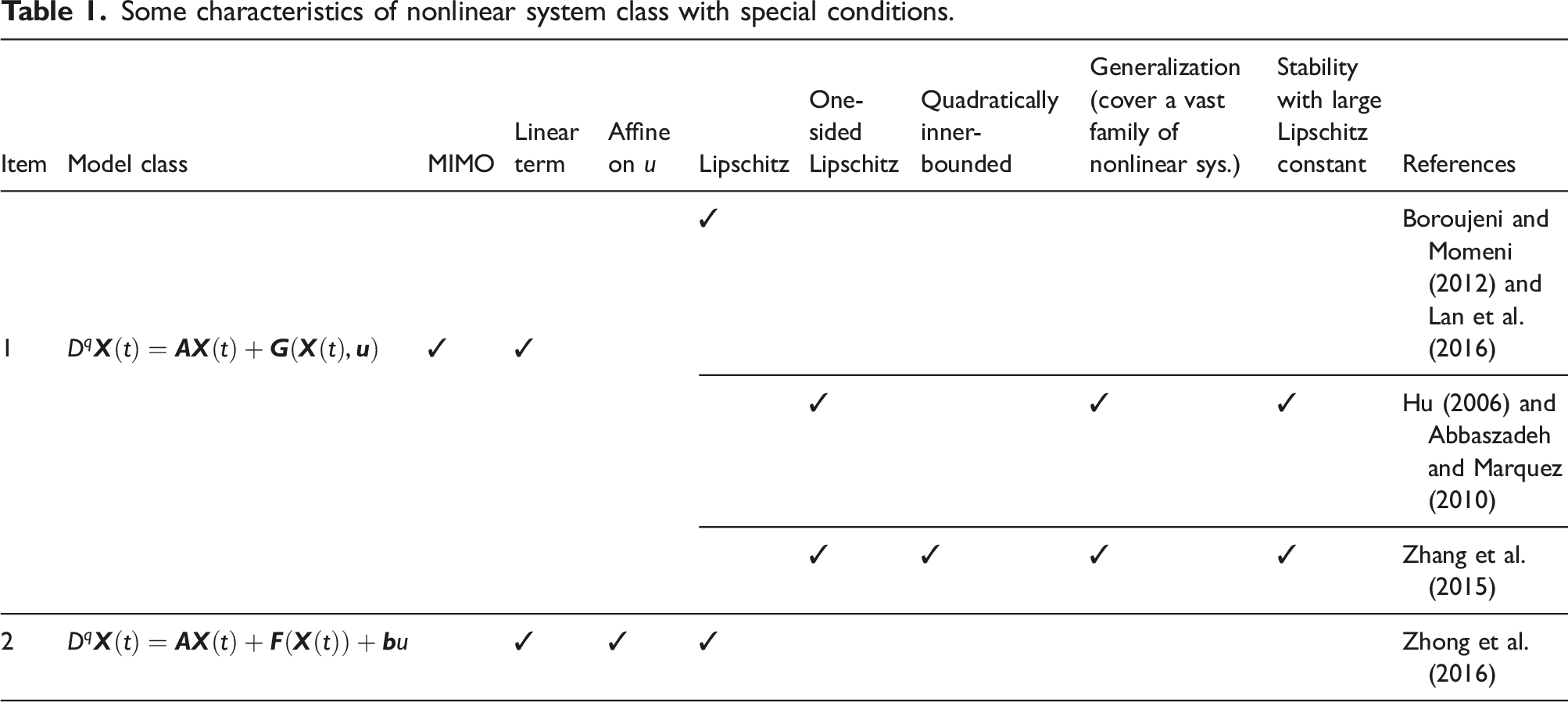
Recently, researchers have paid more attention to fractional-order fields. So, several observer design methods for fractional-order (FO) linear and nonlinear systems have been introduced during the latest years. For example, an observer in the form of FO has been presented in NDoye et al. (2013), applied on a FO linear system with unknown input. Moreover, in Liu and Laleg (2015); Rapaic and Alessandro (2014), adaptive observers have been introduced for a FO linear system. The so-called non-fragile observer for FO nonlinear systems has been studied in Boroujeni and Momeni (2012); Jeong et al. (2006); Lan and Zhou (2013). In the latter studies, the term the fragile or non-resilient observer has been referred to as divergence of estimation error, which may be resulted from a minor disturbance in observer gain. In Hafezi et al. (2020); N’Doye et al. (2013); Senejohnny and Delavari (2012), observer-based synchronization has been suggested for FO chaotic systems. Lipschitz nonlinear systems are a popular class of nonlinear systems considered in some studies (Lan et al., 2016; Zhong et al., 2016). Recently, more attention has been paid to this class of nonlinear systems. Despite their efficacy, the Lipschitz type of nonlinear systems suffers from minor and/or large values of the Lipschitz constants that may render linear matrix inequalities (LMIs) infeasible and cause the designed observer to be unstable (Lan and Zhou, 2013). To overcome this limitation, well-known one-sided Lipschitz condition and quadratically inner-bounded requirement have been introduced in Abbaszadeh and Marquez (2010); Abdullah and Qasem (2019); Hu (2006); Zhang et al. (2015); Zulfiqar et al. (2016). Some characteristics of nonlinear systems with those conditions are listed in Table 1.

Table 1.

Some characteristics of nonlinear system class with special conditions.

Item	Model class	MIMO	Linear term	Affine on $u$	Lipschitz	One-sided Lipschitz	Quadratically inner-bounded	Generalization (cover a vast family of nonlinear sys.)	Stability with large Lipschitz constant	References
1	$D^q\mathit{X}\left(t\right)=\mathit{A}\mathit{X}\left(t\right)+\mathit{G}\left(\mathit{X}\left(t\right),\mathit{u}\right)$	✓	✓		✓					Boroujeni and Momeni (2012) and Lan et al. (2016)
											✓		✓	✓	Hu (2006) and Abbaszadeh and Marquez (2010)
											✓	✓	✓	✓	Zhang et al. (2015)
2	$D^q\mathit{X}\left(t\right)=\mathit{A}\mathit{X}\left(t\right)+\mathit{F}\left(\mathit{X}\left(t\right)\right)+\mathit{b}u$		✓	✓	✓					Zhong et al. (2016)

Recently, some researchers have shown a particular interest in the well-known differential mean value theorem (DMVT), which is less conservative than the methods as mentioned above (Sharma et al., 2016, 2018; Zemouche and Boutayeb, 2009, 2013; Zemouche et al., 2005, 2008). By this theorem, dynamics of observation error with nonlinear terms are converted into linear parameter-varying (LPV) dynamics. Stability analysis of the method is easy, and one can investigate simply using a classical quadratic Lyapunov function and convexity theory. Convergence of estimation states to nominal states is guaranteed by feasibility and existence of a solution for LMI conditions, providing the observer gain.

In the case of observer design, a general affine class of nonlinear FO systems already studied includes systems in the form of $D^q\mathit{X}(t)=\mathit{f}(\mathit{X})+\mathit{b}u$ , where b is the constant vector (gain of the system input) and $u$ is the scalar input. Having this fact in mind, to the best of our knowledge, none of the previous studies have investigated an affine nonlinear single-input/single-output (SISO) or multi-input/multi-output (MIMO) system, in which gain of the system input is a nonlinear function of the states’ vector, that is, a system in the form of $D^q\mathit{X}(t)=\mathit{f}(\mathit{X})+\mathit{G}(\mathit{X})\mathit{u}$ . However, in this paper, first of all, a new FO observer is proposed for FO nonlinear MIMO systems in the last mentioned form. Then, using DMVT, the dynamic equation of state observation error is converted into an LPV dynamic system. Finally, observer gains of the proposed method are obtained by suggesting a Lyapunov function and solving some LMI problems, ensuring asymptotic stability and convergence of the observation error.

The rest of this paper is organized as follows. At first, a brief overview of some definitions and properties of fractional calculus is given in Section 2. The problem is stated in Section 3. The fourth section is concerned with the methodology proposed in this paper. The fifth section presents the research findings, focusing on illustrations regarding the performance of the proposed observer through some examples. Finally, a summary and evaluation of the results are presented in the Conclusion section.

2. Preliminaries on fractional calculus

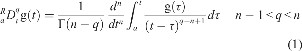
In this section, some definitions, properties, and theorems found in the field of fractional calculus are described. The first definition is a fractional derivative of order $q$ of a function $\mathrm{g}(t)$ , introduced by Riemann–Liouville (Valério et al., 2013)

${{}_a{}^{R}D}_t^q\mathrm{g}(t)=\frac{1}{\mathrm{\Gamma }(n-q)}\frac{d^n}{{dt}^n}{\int }_a^t\frac{\mathrm{g}(\tau )}{{(t-\tau )}^{q-n+1}}d\tau \hspace{0.17em}n-1<q<n$

(1)

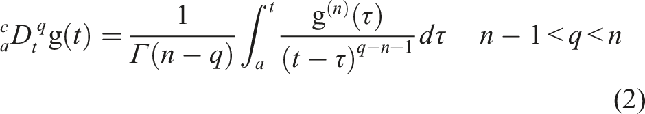
The second definition is the fractional derivative presented by Caputo (Valério et al., 2013)

${{}_a{}^{c}D}_t^q\mathrm{g}(t)=\frac{1}{\Gamma (n-q)}{\int }_a^t\frac{{\mathrm{g}}^{(n)}(\tau )}{{(t-\tau )}^{q-n+1}}d\tau \hspace{0.17em}n-1<q<n$

(2)

where $n\in N,\hspace{0.17em}q\in R^{+}$ , and Gamma function $\Gamma (.)$ is defined as $\Gamma (\tau )={\int }_0^{\infty }{e}^{-t}{t}^{\tau -1}dt$ .

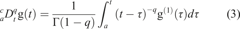
In particular, if $0<q<1$ , then

${{}_a{}^{c}D}_t^q\mathrm{g}(t)=\frac{1}{\mathrm{\Gamma }(1-q)}{\int }_a^t{(t-\tau )}^{-q}{\mathrm{g}}^{(1)}(\tau )d\tau$

(3)

Interestingly, in the latter definition, there is a similarity between the description of the initial conditions for FO equations and integer-order ones (Sharma et al., 2018). Therefore, although researchers suggested various specification of the fractional derivative term, the Caputo derivative definition will be used in this paper.

Notations

Notations and terminologies introduced throughout this paper are as follows:

1. Transpose of matrix $\mathit{A}$ will be denoted by ${\mathit{A}}^T$ .

2. The notation A > 0 ( A < 0) for a square matrix means positive definition (negative definition) of matrix A .

3. The convex hull of $\left\{\mathit{x},\mathit{y}\right\}\in R^n$ , denoted by the $Conv(\mathit{x},\mathit{y})$ , is defined as the $Conv(\mathit{x},\mathit{y})=\left\{\lambda \mathit{x}+(1-\lambda )\mathit{y},\hspace{0.17em}0\le \lambda \le 1\right\}$ .

4. ${\mathit{\xi }}_n(i)={(0,\dots ,0,\underset{i}{\underset{\{}{1}},0,\dots ,0)}^T\in R^n,\hspace{0.17em}n\ge 1,\hspace{0.17em}i=1,\dots ,n$ implies a vector of canonical basis of $R^n$ .

Theorem 1

(Aguila et al., 2014; Chen et al., 2014): (Lyapunov stability of FO systems) Consider the FO dynamic system as

$D^q\mathit{X}=\mathit{f}(\mathit{X})$

(4)

where $\mathit{X}={\left[x_1,x_2,\dots ,x_n\right]}^T\in R^n$ is the state vector. $\mathit{f}(\mathit{X}):R^n\to R^n$ is a smooth nonlinear function in a vector form. The FO is represented by $q\in (0,1]$ . Nonlinear system (4) is asymptotically stable if it is found that a Lyapunov function $V(\mathit{X})>0$ , such that $D^{q}V(\mathit{X})<0$ for all $t\ge 0$ .

Theorem 2

(Duarte-Mermoud et al., 2014): Consider $\mathit{X}(t)\in {\mathbb{R}}^n$ to be a differentiable function vector and $\mathit{P}\in {\mathbb{R}}^{n\times n}$ to be a constant matrix in a symmetric positive definite form. Then, the following inequality is satisfied

$\frac{1}{2}{D}^q({\mathit{X}}^T(t)\mathit{P}\mathit{X}(t))\le {\mathit{X}}^T(t)\mathit{P}\hspace{0.17em}(D^q\mathit{X}(t))$

(5)

where $q\in (\mathrm{0,1}],\hspace{0.17em}t\ge t_0$ .

Lemma 1

(Sharma et al., 2016, 2018; Zemouche and Boutayeb, 2009, 2013; Zemouche et al., 2005, 2008): (DMVT technique) Let $\mathbf{\Lambda }(\mathrm{\nu })\hspace{0.17em}:\hspace{0.17em}{\mathbb{R}}^n\to {\mathbb{R}}^m$ and $\mathit{\sigma },\hspace{0.17em}\mathit{\theta }\in {\mathbb{R}}^n$ so that $\mathbf{\Lambda }(\mathrm{\nu })$ is differentiable on $Conv(\mathit{\sigma },\hspace{0.17em}\mathit{\theta })$ . Then, there are constant vectors ${\mathit{\eta }}_1,\dots ,{\mathit{\eta }}_m\in Conv(\mathit{\sigma },\hspace{0.17em}\mathit{\theta }),\hspace{0.17em}{\mathit{\eta }}_i\ne \mathit{\sigma },\hspace{0.17em}{\mathit{\eta }}_i\ne \mathit{\theta }$ for $i=1,\dots ,m$ , such that

$\mathbf{\Lambda }(\mathit{\sigma })-\mathbf{\Lambda }(\mathit{\theta })=({\displaystyle \sum }_{i,j=1}^{m,n}{\mathit{\xi }}_m(i){\mathit{\xi }}_n^T(j)\frac{\partial {\mathbf{\Lambda }}_i}{\partial {\mathrm{\nu }}_i}({\mathit{\eta }}_i))(\mathit{\sigma }-\mathit{\theta })$

(6)

where ${\mathit{\xi }}_m(i)$ is a vector of the canonical basis of $R^n$ .

3. Problem formulation

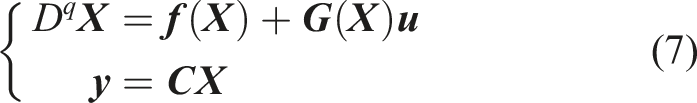
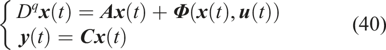
A general affine class of FO nonlinear dynamic systems in the form of state space can be considered as

$\{\begin{array}{c}{D}^q\mathit{X}=\mathit{f}(\mathit{X})+\mathit{G}(\mathit{X})\mathit{u}\\ \mathit{y}=\mathit{C}\mathit{X}\hspace{0.17em}\end{array}$

(7)

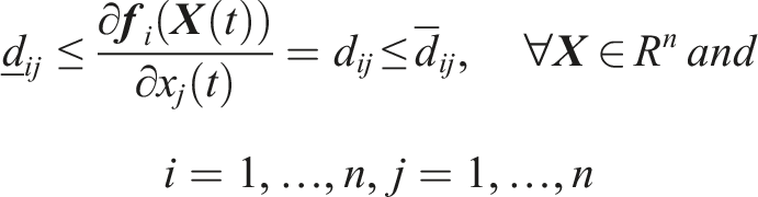
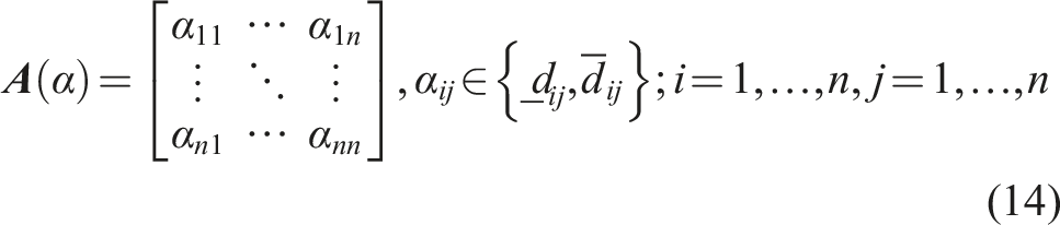
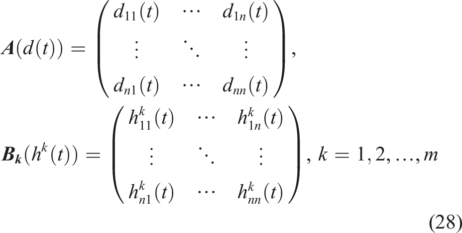
where $\mathit{X}={\left[x_1,x_2,\dots ,x_n\right]}^T\in R^n$ is the state vector, $\mathit{u}\in R^m$ is the input, $\mathit{y}\in R^p$ is the output, that is, the measurable output variables of the system, $\mathit{C}$ is the matrix with appropriate dimensions, that is, $\mathit{C}\in R^{p\times n}$ , $\mathit{f}(\mathit{X})\in R^n$ is the nonlinear function vector, and $\mathit{G}(\mathit{X})=\left[{\mathbf{g}}_1(\mathit{X}),\hspace{0.17em}\dots ,{\mathbf{g}}_m(\mathit{X})\right]\in R^{n\times m}$ is the nonlinear function matrix, both of which are supposed to be known and differentiable. The fractional order is represented by $q\in (\mathrm{0,1})$ .

Assumption 1

(Sharma et al., 2016, 2018; Zemouche and Boutayeb, 2009, 2013; Zemouche et al., 2005, 2008). It is supposed that the Jacobean matrix of $\mathit{f}(\mathit{X})$ and $\mathit{G}(\mathit{X})=\left[{\mathbf{g}}_1(\mathit{X}),\hspace{0.17em}\dots ,{\mathbf{g}}_m(\mathit{X})\right]$ meet the subsequent conditions

${\underset{\_}{d}}_{ij}\le \frac{\partial {\mathit{f}}_i(\mathit{X}(t))}{\partial x_j(t)}=d_{ij}\le {\overline{d}}_{ij},\forall \mathit{X}\in R^n\hspace{0.17em}and\hspace{0.17em}i=1,\dots ,n,\hspace{0.17em}j=1,\dots ,n$

${\underset{\_}{\underset{\_}{h}}}_{ij}^k\le \frac{\partial {\mathbf{g}}_i^k(\mathit{X}(t))}{\partial x_j(t)}=h_{ij}^k\le {\overline{h}}_{ij}^k,\forall \mathit{X}\in R^n\hspace{0.17em}and\hspace{0.17em}i=1,\dots ,n;\hspace{0.17em}j=1,\dots ,n\hspace{0.17em};\hspace{0.17em}k=1,\dots ,m$

(8)

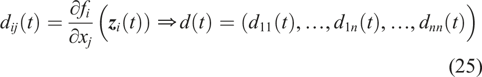
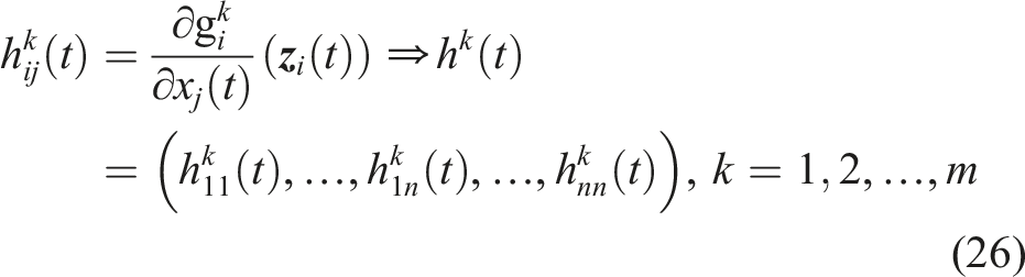
where ${\mathit{f}}_i(\mathit{X})$ is the i-th row of function vector $\mathit{f}(\mathit{X})$ and ${\mathbf{g}}_i^k(\mathit{X})$ is the i-th row of column function vector ${\mathbf{g}}_k(\mathit{X})$ , for $k=1,\dots ,m$ . Also, ${\underset{\_}{\underset{\_}{d}}}_{ij}$ , ${\overline{d}}_{ij}$ , ${\underset{\_}{\underset{\_}{d}}}_{ij}^k$ , and ${\overline{h}}_{ij}^k$ are defined as

${\underset{\_}{\underset{\_}{d}}}_{ij}=\underset{\mathit{X}\in {\mathbb{R}}^n}{\min }(\frac{\partial {\mathit{f}}_i(\mathit{X})}{\partial x_j}),\hspace{0.17em}{\overline{d}}_{ij}=\underset{\mathit{X}\in {\mathbb{R}}^n}{\max }(\frac{\partial {\mathit{f}}_i(\mathit{X})}{\partial x_j})$

${\underset{\_}{\underset{\_}{h}}}_{ij}^k=\underset{\mathit{X}\in {\mathbb{R}}^n}{\min }(\frac{\partial {\mathbf{g}}_i^k(\mathit{X})}{\partial x_j}),\hspace{0.17em}{\overline{h}}_{ij}^k=\underset{\mathit{X}\in {\mathbb{R}}^n}{\max }(\frac{\partial {\mathbf{g}}_i^k(\mathit{X})}{\partial x_j})$

(9)

4. Designing the proposed observer

In this section, an observer is proposed for system (7). The observation error dynamic of the proposed method can be evolved as an LPV system by DMVT. Then, a Lyapunov function is introduced to prove the asymptotic convergence of the proposed observer. Stability analysis of the observation error dynamic leads to an LMI problem. Finding a feasible solution for the LMI problem is the final part of this procedure.

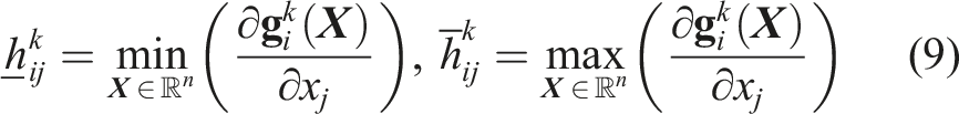
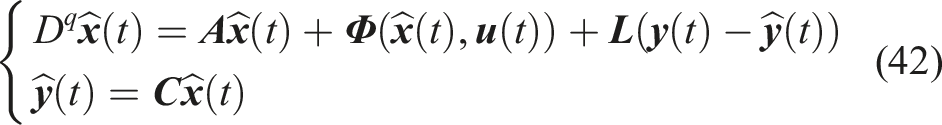
At first, based on the dynamic system introduced by (7), the following FO state observer is proposed

$\{\begin{array}{c}{D}^q\widehat{\mathit{X}}=\mathit{f}(\widehat{\mathit{X}})+\mathit{G}(\widehat{\mathit{X}})\mathit{u}+{\mathit{L}}_0(\mathit{y}-\widehat{\mathit{y}})+{\displaystyle \sum }_{k=1}^m{\mathit{L}}_k(\mathit{y}-\widehat{\mathit{y}})u_k\\ \widehat{\mathit{y}}=\mathit{C}\widehat{\mathit{X}}\hspace{0.17em}\end{array}$

(10)

where $\widehat{\mathit{X}}$ denotes an estimate of the state $\mathit{X}$ . The aim of this study is to determine gain vectors or matrices ${\mathit{L}}_0$ and ${\mathit{L}}_k$ ( $k=1,\dots ,m$ ) such that, the observation error, that is, $\mathit{E}=\mathit{X}-\widehat{\mathit{X}}$ , converges to zero asymptotically.

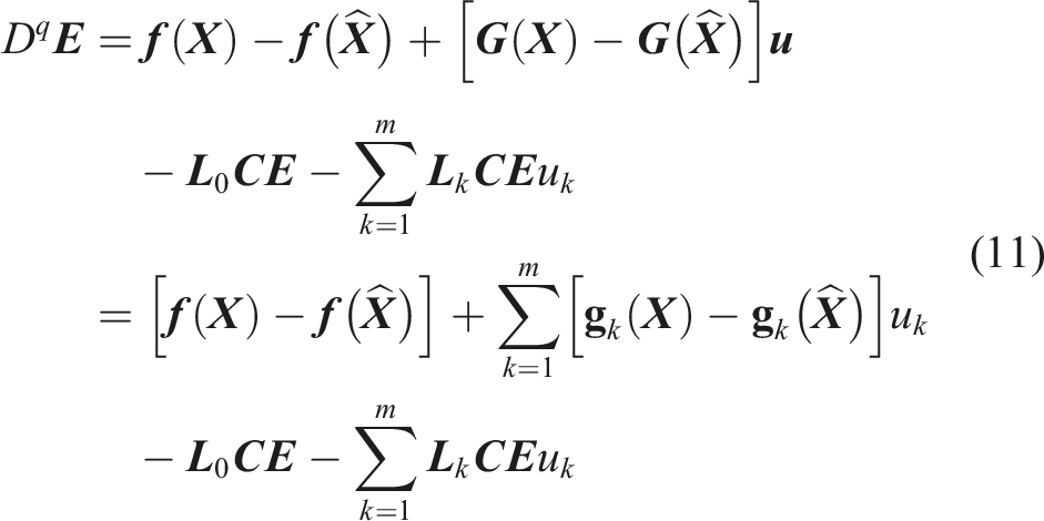
From the definition of the observer error $\mathit{E}$ , system (7), and proposed observer (10), the dynamic of the observation error can be written as

$D^q\mathit{E}=\mathit{f}(\mathit{X})-\mathit{f}(\widehat{\mathit{X}})+\left[\mathit{G}(\mathit{X})-\mathit{G}(\widehat{\mathit{X}})\right]\mathit{u}-{\mathit{L}}_0\mathit{C}\mathit{E}-{\displaystyle \sum }_{k=1}^m{\mathit{L}}_k\mathit{C}\mathit{E}{u}_k=\left[\mathit{f}(\mathit{X})-\mathit{f}(\widehat{\mathit{X}})\right]+{\displaystyle \sum }_{k=1}^m\left[{\mathbf{g}}_k(\mathit{X})-{\mathbf{g}}_k(\widehat{\mathit{X}})\right]u_k-{\mathit{L}}_0\mathit{C}\mathit{E}-{\displaystyle \sum }_{k=1}^m{\mathit{L}}_k\mathit{C}\mathit{E}{u}_k$

(11)

For attaining the convergence of error dynamic (11), a Lyapunov function $V(t)$ is introduced, and based on the feasibility of some LMIs, it can be assured that $D^{q}V<0$ . The observer gain vectors (or matrices), that is, ${\mathit{L}}_0$ and ${\mathit{L}}_k\hspace{0.17em}(k=1,\dots ,m)$ , can be calculated through the feasibility of the LMIs.

Herein, some preliminaries are presented before proceeding to the proposed approach. Firstly, based on assumption 1, it will be necessary to introduce the sets $D_{n,n}$ and $H_{n,n}^k$ as follows (Sharma et al., 2016, 2018; Zemouche and Boutayeb, 2009; Zemouche et al., 2008)

$D_{n,n}=\left\{d=(d_{11},\hspace{0.17em}\dots ,\hspace{0.17em}{d}_{1n},\dots ,d_{nn}):\hspace{0.17em}{\underset{\_}{d}}_{ij}\le d_{ij}\le {\overline{d}}_{ij},\hspace{0.17em}i=1,\dots ,n;\hspace{0.17em}j=1,\dots ,n\right\}$

$H_{n,n}^k=\left\{h^k=(h_{11}^k,\hspace{0.17em}\dots ,\hspace{0.17em}{h}_{1n}^k,\dots ,h_{nn}^k):\hspace{0.17em}{\underset{\_}{\underset{\_}{h}}}_{ij}^k\le h_{ij}^k\le {\overline{h}}_{ij}^k,\hspace{0.17em}i=1,\dots ,n;\hspace{0.17em}j=1,\dots ,n\right\},\hspace{0.17em}k=1,\dots ,m$

(12)

The sets $D_{n,n}$ and $H_{n,n}^k$ are two bounded convex domains of $2^{(n^2)}$ vertices. These vertices are defined for each set as follows

${\mathcal{V}}_{D_{n,n}}=\left\{\alpha =\left\{{\alpha }_{11},\hspace{0.17em}\dots ,\hspace{0.17em}{\alpha }_{1n},\dots ,{\alpha }_{nn}\right\}:\hspace{0.17em}{\alpha }_{ij}\in \left\{{\underset{\_}{\underset{\_}{d}}}_{ij},{\overline{d}}_{ij}\right\}\hspace{0.17em}\right\}$

${\mathcal{V}}_{H_{n,n}^k}=\left\{{\beta }^k=\left\{{\beta }_{11}^k,\hspace{0.17em}\dots ,\hspace{0.17em}{\beta }_{1n}^k,\dots ,{\beta }_{nn}^k\right\}:\hspace{0.17em}{\beta }_{ij}^k\in \left\{{\underset{\_}{\underset{\_}{h}}}_{ij}^k,{\overline{h}}_{ij}^k\right\}\hspace{0.17em}\right\},\hspace{0.17em}k=1,\dots ,m$

(13)

Based on $\mathit{f}(\mathit{X})$ and $\mathit{G}(\mathit{X})=\left[{\mathbf{g}}_1(\mathit{X}),\hspace{0.17em}\dots ,{\mathbf{g}}_m(\mathit{X})\right]$ in (7), also (8), (9), and (13), matrices of $\mathit{A}(\alpha )$ and ${\mathit{B}}_k({\beta }^k)$ are defined as (Sharma et al., 2016, 2018; Zemouche and Boutayeb, 2009; Zemouche et al., 2008)

$\mathit{A}(\alpha )=\left[\begin{array}{ccc}{\alpha }_{11}& \cdots & {\alpha }_{1n}\\ ⋮& \ddots & ⋮\\ {\alpha }_{n1}& \cdots & {\alpha }_{nn}\end{array}\right],\hspace{0.17em}{\alpha }_{ij}\in \left\{{\underset{\_}{\underset{\_}{d}}}_{ij},{\overline{d}}_{ij}\right\};\hspace{0.17em}i=1,\dots ,n,\hspace{0.17em}j=1,\dots ,n$

(14)

${\mathit{B}}_k({\beta }^k)=\left[\begin{array}{ccc}{\beta }_{11}^k& \cdots & {\beta }_{1n}^k\\ ⋮& \ddots & ⋮\\ {\beta }_{n1}^k& \cdots & {\beta }_{nn}^k\end{array}\right],\hspace{0.17em}{\beta }_{ij}^k\in \left\{{\underset{\_}{\underset{\_}{h}}}_{ij}^k,{\overline{h}}_{ij}^k\right\};\hspace{0.17em}i=1,\dots ,n,\hspace{0.17em}j=1,\dots ,n,\hspace{0.17em}k=1,\dots ,m$

(15)

The following theorem is the key to presenting the previous results, followed by its proof.

Theorem 3

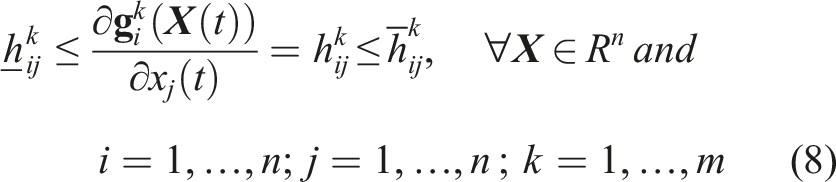
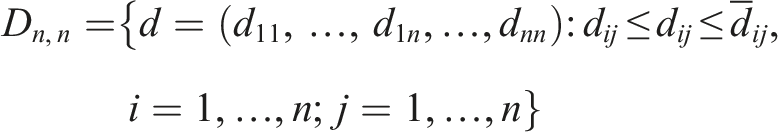
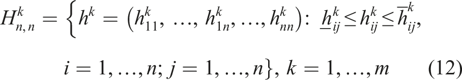
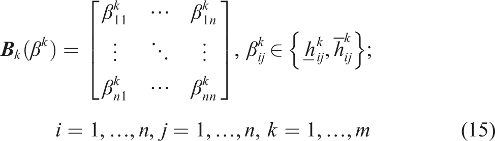
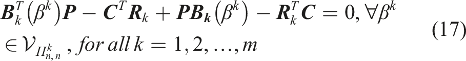
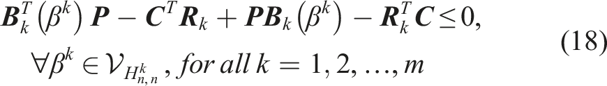
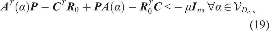
Consider the dynamic system (7) and observer (10). For every matrices $\mathit{P}={\mathit{P}}^T>0$ , ${\mathit{R}}_0$ , ${\mathit{R}}_k\hspace{0.17em}(k=1,\dots ,m)$ , and $\mathit{A}(\alpha )$ and ${\mathit{B}}_{\mathit{k}}({\beta }^k)$ , which are defined based on (14) and (15), respectively, the observers’ error $\mathit{E}$ will converge to zero asymptotically for all $\alpha \in {\mathcal{V}}_{D_{n,n}}$ and ${\beta }^k\in {\mathcal{V}}_{H_{n,n}^k}$ (defined in (13)), if one of the following three cases are fulfilled.

Case 1

If the subsequent LMIs are satisfied

${\mathit{A}}^T(\alpha )\mathit{P}-{\mathit{C}}^T{\mathit{R}}_0+\mathit{P}\mathit{A}(\alpha )-{\mathit{R}}_0^T\mathit{C}<0,\forall \alpha \in {\mathcal{V}}_{D_{n,n}}$

(16)

and succeeding equalities are held

${\mathit{B}}_k^T({\beta }^k)\mathit{P}-{\mathit{C}}^T{\mathit{R}}_k+\mathit{P}{\mathit{B}}_{\mathit{k}}({\beta }^k)-{\mathit{R}}_k^T\mathit{C}=0,\forall {\beta }^k\in {\mathcal{V}}_{H_{n,n}^k}\hspace{0.17em},\hspace{0.17em}for\hspace{0.17em}all\hspace{0.17em}k=\mathrm{1,2},\dots ,m$

(17)

Case 2

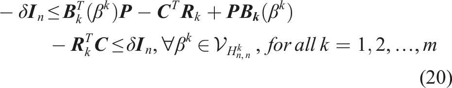
If the following LMIs are satisfied

${\mathit{A}}^T(\alpha )\mathit{P}-{\mathit{C}}^T{\mathit{R}}_0+\mathit{P}\mathit{A}(\alpha )-{\mathit{R}}_0^T\mathit{C}<0,\forall \alpha \in {\mathcal{V}}_{D_{n,n}}$

${\mathit{B}}_k^T({\beta }^k)\mathit{P}-{\mathit{C}}^T{\mathit{R}}_k+\mathit{P}{\mathit{B}}_k({\beta }^k)-{\mathit{R}}_k^T\mathit{C}\le 0,\forall {\beta }^k\in {\mathcal{V}}_{H_{n,n}^k\hspace{0.17em}},\hspace{0.17em}for\hspace{0.17em}all\hspace{0.17em}k=\mathrm{1,2},\dots ,m$

(18)

in addition, $u_k\ge 0$ , for all $k=\mathrm{1,2},\dots ,m$ .

Case 3

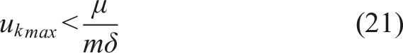
If there are two positive constants $\mu$ and $\delta$ such that the following inequalities are satisfied

${\mathit{A}}^T(\alpha )\mathit{P}-{\mathit{C}}^T{\mathit{R}}_0+\mathit{P}\mathit{A}(\alpha )-{\mathit{R}}_0^T\mathit{C}<-\mu {\mathit{I}}_n,\forall \alpha \in {\mathcal{V}}_{D_{n,n}}$

(19)

$-\delta {\mathit{I}}_n\le {\mathit{B}}_k^T({\beta }^k)\mathit{P}-{\mathit{C}}^T{\mathit{R}}_k+\mathit{P}{\mathit{B}}_{\mathit{k}}({\beta }^k)-{\mathit{R}}_k^T\mathit{C}\le \delta {\mathit{I}}_n,\forall {\beta }^k\in {\mathcal{V}}_{H_{n,n}^k}\hspace{0.17em},\hspace{0.17em}for\hspace{0.17em}all\hspace{0.17em}k=\mathrm{1,2},\dots ,m$

(20)

and also

${u_k}_{\mathit{max}}<\frac{\mu }{m\delta }$

(21)

where ${\mathit{I}}_n$ is $n\times n$ identity matrix and

${u_k}_{\mathit{max}}=\underset{k}{\mathit{max}}(\underset{t\ge 0}{\mathit{sup}}\left|u_k(t)\right|),\hspace{0.17em}k=\mathrm{1,2},\dots m$

(22)

In each case, the matrices ${\mathit{L}}_0$ and ${\mathit{L}}_k\hspace{0.17em}(k=1,\dots ,m)$ are obtained by ${\mathit{L}}_0={\mathit{P}}^{-1}{\mathit{R}}_0^T$ and ${\mathit{L}}_k={\mathit{P}}^{-1}{\mathit{R}}_k^T$ , respectively.

Proof

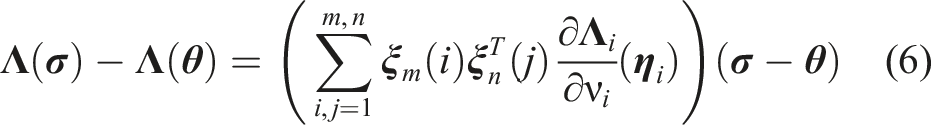
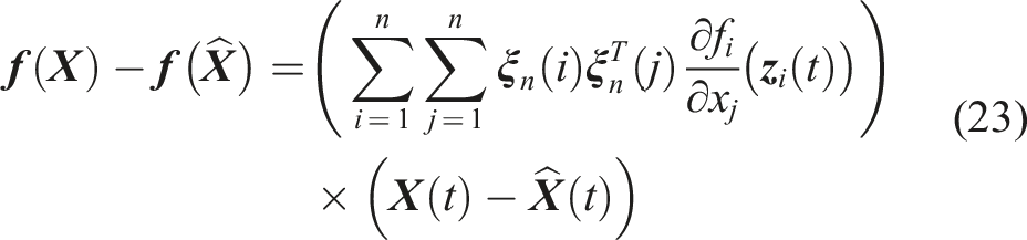
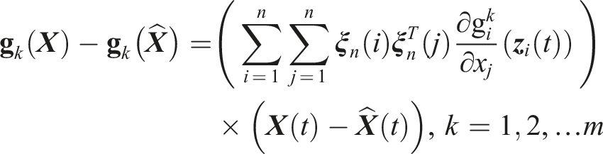
The nonlinear terms in observation error dynamic (11) take form through the use of DMVT technique (Lemma 1)

$\mathit{f}(\mathit{X})-\mathit{f}(\widehat{\mathit{X}})=({\displaystyle \sum }_{i=1}^n{\displaystyle \sum }_{j=1}^n{\mathit{\xi }}_n(i){\mathit{\xi }}_n^T(j)\frac{\partial f_i}{\partial x_j}({\mathit{z}}_i(t)))(\mathit{X}(t)-\widehat{\mathit{X}}(t))$

(23)

${\mathbf{g}}_k(\mathit{X})-{\mathbf{g}}_k(\widehat{\mathit{X}})=({\displaystyle \sum }_{i=1}^n{\displaystyle \sum }_{j=1}^n{\mathit{\xi }}_n(i){\mathit{\xi }}_n^T(j)\frac{\partial {\mathrm{g}}_i^k}{\partial x_j}({\mathit{z}}_i(t))\hspace{0.17em})(\mathit{X}(t)-\widehat{\mathit{X}}(t)),\hspace{0.17em}k=\mathrm{1,2},\dots m$

where ${\mathit{\xi }}_n(i)$ was introduced earlier in Notation 4 and ${\mathit{z}}_i(t)\in Conv(\mathit{X},\widehat{\mathit{X}})$ .

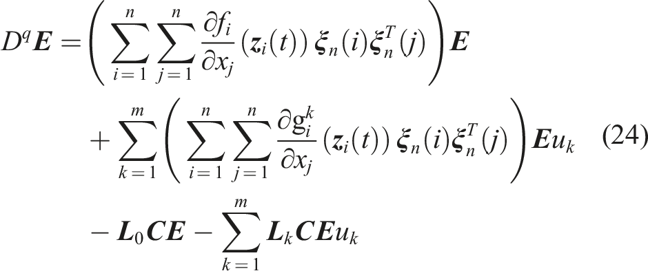
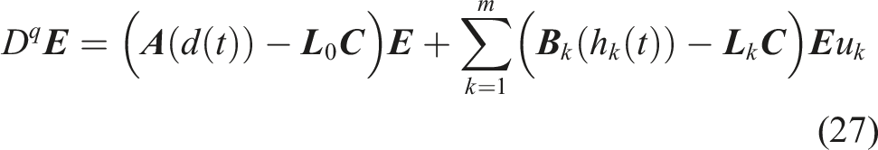
Now, utilizing (23), error dynamic (11) can be written in the following form

$D^q\mathit{E}=({\displaystyle \sum }_{i=1}^n{\displaystyle \sum }_{j=1}^n\frac{\partial f_i}{\partial x_j}({\mathit{z}}_i(t))\hspace{0.17em}{\mathit{\xi }}_n(i){\mathit{\xi }}_n^T(j))\mathit{E}+{\displaystyle \sum }_{k=1}^m({\displaystyle \sum }_{i=1}^n{\displaystyle \sum }_{j=1}^n\frac{\partial {\mathrm{g}}_i^k}{\partial x_j}({\mathit{z}}_i(t))\hspace{0.17em}{\mathit{\xi }}_n(i){\mathit{\xi }}_n^T(j))\mathit{E}{u}_k-{\mathit{L}}_0\mathit{C}\mathit{E}-{\displaystyle \sum }_{k=1}^m{\mathit{L}}_k\mathit{C}\mathit{E}{u}_k$

(24)

Using the following notations

$d_{ij}(t)=\frac{\partial f_i}{\partial x_j}({\mathit{z}}_i(t))\hspace{0.17em}\Rightarrow d(t)=(d_{11}(t),\dots ,d_{1n}(t),\dots ,d_{nn}(t))$

(25)

$h_{ij}^k(t)=\frac{\partial {\mathrm{g}}_i^k}{\partial x_j(t)}({\mathit{z}}_i(t))\hspace{0.17em}\Rightarrow h^k(t)=(h_{11}^k(t),\dots ,h_{1n}^k(t),\dots ,h_{nn}^k(t)),\hspace{0.17em}k=\mathrm{1,2},\dots ,m$

(26)

Error dynamic (24) can be substituted by

$D^q\mathit{E}=(\mathit{A}(d(t))-{\mathit{L}}_0\mathit{C})\mathit{E}+{\displaystyle \sum }_{k=1}^m({\mathit{B}}_k(h_k(t))-{\mathit{L}}_k\mathit{C})\mathit{E}{u}_k\hspace{0.17em}$

(27)

where

$\mathit{A}(d(t))=(\begin{array}{ccc}{d}_{11}(t)& \cdots & d_{1n}(t)\\ ⋮& \ddots & ⋮\\ d_{n1}(t)& \cdots & d_{nn}(t)\end{array}),\hspace{0.17em}{\mathit{B}}_{\mathit{k}}(h^k(t))=(\begin{array}{ccc}{h}_{11}^k(t)& \cdots & h_{1n}^k(t)\\ ⋮& \ddots & ⋮\\ h_{n1}^k(t)& \cdots & h_{nn}^k(t)\end{array}),\hspace{0.17em}k=\mathrm{1,2},\dots ,m$

(28)

Error dynamic (27) is an LPV system, that is, using DMVT (Zemouche et al., 2008), the observation error dynamic is transformed into an LPV system. Now, a Lyapunov function candidate is chosen as

$V(t)={\mathit{E}}^{\mathit{T}}(t)\mathit{P}\mathit{E}(t)$

(29)

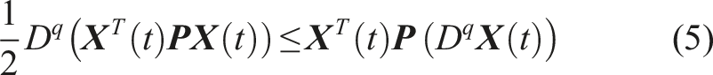
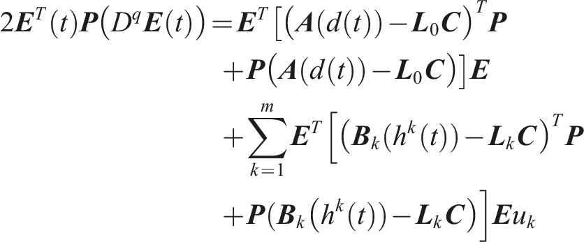
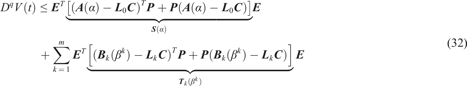
where $\mathit{P}$ is a matrix in a symmetric positive definite form. The following inequality can be held by fractional differentiating concerning time using (29) and regarding (5)

$D^{q}V(t)\le 2{\mathit{E}}^T(t)\mathit{P}(D^q\mathit{E}(t))$

(30)

The right-hand side of equation (30) can be written as

$2{\mathit{E}}^T(t)\mathit{P}\left(D^q\mathit{E}(t)\right)={\mathit{E}}^T(t)\mathit{P}(D^q\mathit{E}(t))+{(D^q\mathit{E}(t))}^T\mathit{P}\mathit{E}(t)$

Then, by substituting (27) in right-hand side of the latter, we have

$2{\mathit{E}}^T(t)\mathit{P}(D^q\mathit{E}(t))={\mathit{E}}^T\left[{(\mathit{A}(d(t))-{\mathit{L}}_0\mathit{C})}^T\mathit{P}+\mathit{P}(\mathit{A}(d(t))-{\mathit{L}}_0\mathit{C})\right]\mathit{E}+{\displaystyle \sum }_{k=1}^m{\mathit{E}}^T\left[{({\mathit{B}}_k(h^k(t))-{\mathit{L}}_k\mathit{C})}^T\mathit{P}+\mathit{P}({\mathit{B}}_k(h^k(t))-{\mathit{L}}_k\mathit{C})\right]\mathit{E}{u}_k$

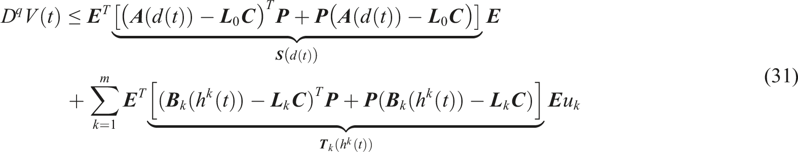
Thus, according to FO differential inequality (30), one can obtain

$D^{q}V(t)\le {\mathit{E}}^T\underset{\mathit{S}(d(t))}{\underbrace{\left[{(\mathit{A}(d(t))-{\mathit{L}}_0\mathit{C})}^T\mathit{P}+\mathit{P}(\mathit{A}(d(t))-{\mathit{L}}_0\mathit{C})\right]}}\mathit{E}+{\displaystyle \sum }_{k=1}^m{\mathit{E}}^T\underset{{\mathit{T}}_k(h^k(t))}{\underbrace{\left[{({\mathit{B}}_k(h^k(t))-{\mathit{L}}_k\mathit{C})}^T\mathit{P}+\mathit{P}({\mathit{B}}_k(h^k(t))-{\mathit{L}}_k\mathit{C})\right]}}\mathit{E}{u}_k$

(31)

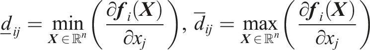
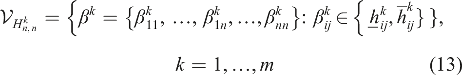
Based on Assumption 1 and equations (25) and (26), the parameters $d_{ij}$ and $h_{ij}^k$ are bounded for each i, j, and $k=1,\dots ,m$ . Thus, $d(t)$ and $h^k(t)$ lie in a bounded domain. The matrix functions ${\mathit{T}}_k(.)$ and $\mathit{S}(.)$ in (31) are affined in $d(t)$ and $h^k(t)$ , respectively. Thus using the convexity principle (Boyd and Vandenberghe, 2001), if by the matrices $\mathit{A}(\alpha )$ and ${\mathit{B}}_k({\beta }^k)$ (such as (14) and (15)), the matrix functions ( ${\mathit{T}}_k(.)$ and $\mathit{S}(.)$ ) are satisfied at the vertices ${\mathcal{V}}_{D_{n,n}}$ and ${\mathcal{V}}_{H_{n,n}^k}$ (such as (13)), it is deduced that for all values of $d(t)$ and $h^k(t)$ , the matrix functions ( ${\mathit{T}}_k(.)$ and $\mathit{S}(.)$ ) will lie in bounded domains as $D_{n,n}$ and $H_{n,n}^k$ (such as (12)), respectively. Consequently, noticing (31), one can result

$D^{q}V(t)\le {\mathit{E}}^T\underset{\mathit{S}(\alpha )}{\underbrace{\left[{(\mathit{A}(\alpha )-{\mathit{L}}_0\mathit{C})}^T\mathit{P}+\mathit{P}(\mathit{A}(\alpha )-{\mathit{L}}_0\mathit{C})\right]}}\mathit{E}+{\displaystyle \sum }_{k=1}^m{\mathit{E}}^T\underset{{\mathit{T}}_k({\beta }^k)}{\underbrace{\left[{({\mathit{B}}_k({\beta }^k)-{\mathit{L}}_k\mathit{C})}^T\mathit{P}+\mathit{P}({\mathit{B}}_k({\beta }^k)-{\mathit{L}}_k\mathit{C})\right]}}\mathit{E}$

(32)

According to (32), if (16) and (17), that is, Cases 1 and 2 are satisfied, then $D^{q}V(t)<0$ . Also provided that (18) and $u_k\ge 0$ , for all $k=\mathrm{1,2},\dots ,m$ are pleased, it follows that asymptotic stability and zero convergence of the observer error $\mathit{E}$ are concluded, that is, $D^{q}V(t)<0$ .

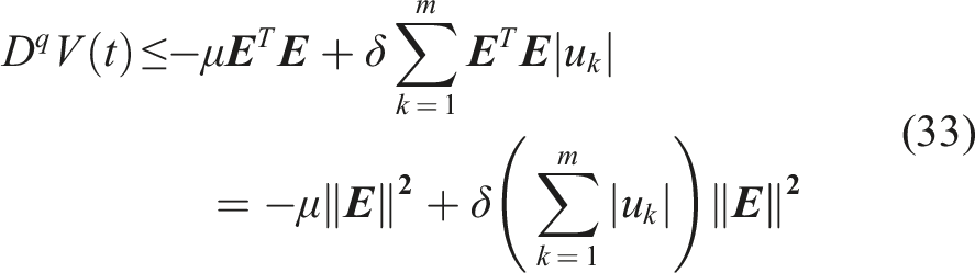
In Case 3, considering (19), (20), and (32), one can write

$D^{q}V(t)\le -\mu {\mathit{E}}^T\mathit{E}+\delta {\displaystyle \sum }_{k=1}^m{\mathit{E}}^T\mathit{E}\left|u_k\right|=-\mu {\Vert \mathit{E}\Vert }^{\mathbf{2}}+\delta ({\displaystyle \sum }_{k=1}^m\left|u_k\right|){\Vert \mathit{E}\Vert }^{\mathbf{2}}$

(33)

Noticing (22), one sufficient condition for satisfying (33) is

$D^{q}V(t)\le (-\mu +\delta \hspace{0.17em}m\hspace{0.17em}{u_k}_{\mathit{max}}){\Vert \mathit{E}\Vert }^{\mathbf{2}}$

(34)

Now, if ${u_k}_{\mathit{max}}<\frac{\mu }{m\delta }$ is true, it can be concluded that

$D^{q}V(t)<0$

(35)

and the proof is complete.

Remark 1

In many dynamic systems, such as biomedical, process control, positive systems, and also some engineering and economic systems, the control signal must be positive, and therefore, this observer can be used for such systems by noticing Case 2 in the theorem.

Remark 2

Although in Case 3, the proposed observer cannot guarantee asymptotic stability of the observer error for unbounded $\mathit{u}$ , it must be noted that in natural systems, all input signals are always bounded, and therefore, condition (21) may be satisfied by proper selection of $\mu$ and $\delta$ . However, condition (21) is only one of the sufficient conditions for satisfying the theorem in Case 3, whereas the primary satisfactory condition is ${\displaystyle \sum }_{k=1}^m\left|u_k(t)\right|<\frac{\mu }{\delta }\hspace{0.17em},\forall t\ge 0$ , which is less conservative.

Remark 3

The proposed method can be applied to a general affine class of nonlinear integer-order dynamic systems $(q=1)$ , by making a trivial change in the proof procedure.

5. Numerical examples

Three numerical illustrations are presented in this section to show the soundness and usefulness of the recommended design methodology. To show the validity of the suggested scheme, numerical simulations are presented via MATLAB and Simulink environments.

Example 1

The first example is an inverted pendulum mounted on a cart (Atam et al., 2014; Li et al., 2017; Yang et al., 2006). The diagram of the system is represented in Figure 1. The system dynamic is presented by

$\{\begin{array}{l}{D}^q{x}_1(t)=x_2(t)\hspace{0.17em}\\ D^q{x}_2(t)=\frac{g\sin (x_1)-amL{x}_2^2\sin (2x_1)/2-a\cos (x_1)u}{4L/3-amL{\cos }^2(x_1)}\end{array}$

(36)

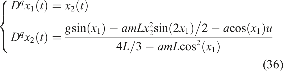
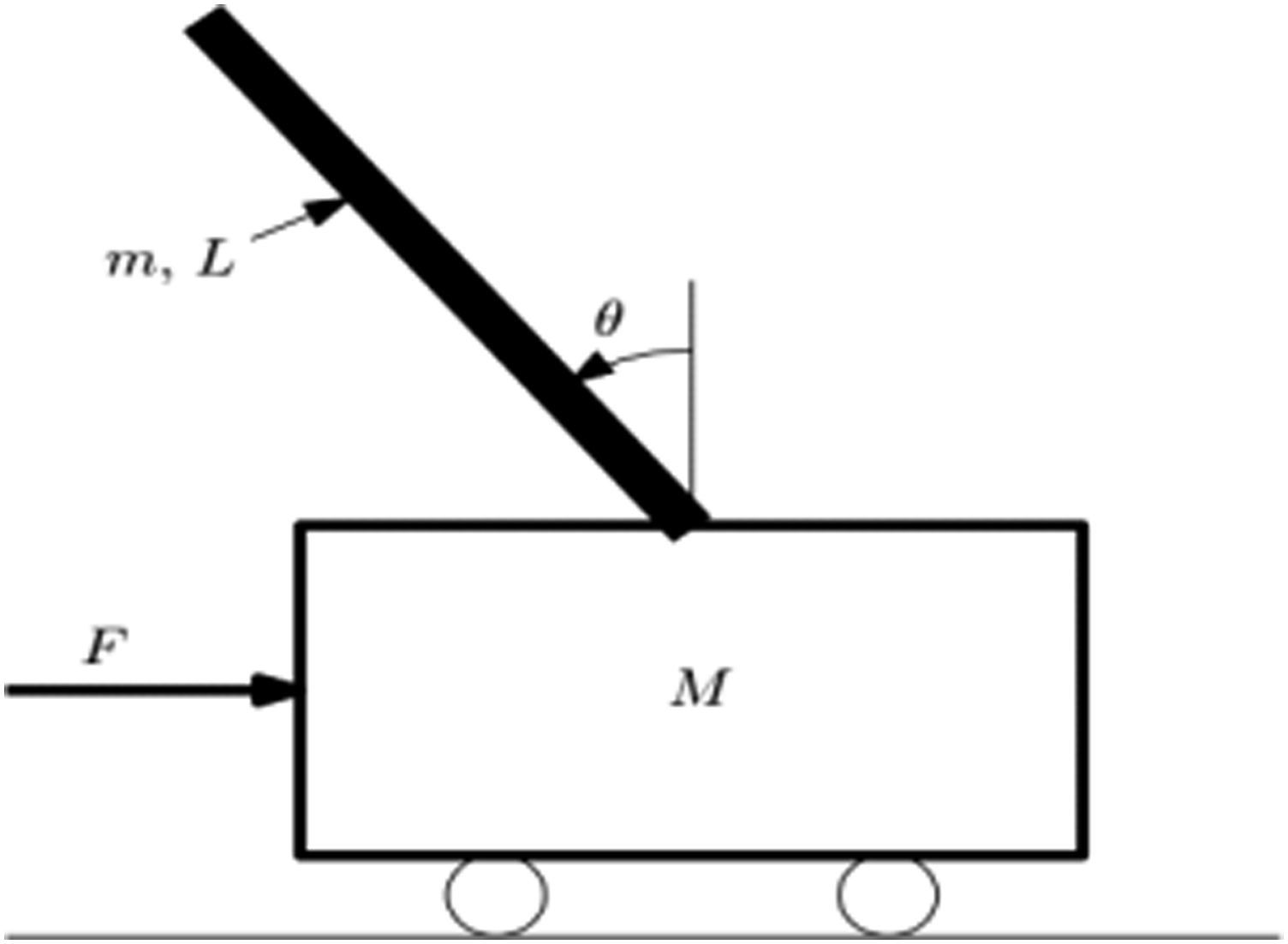
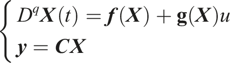
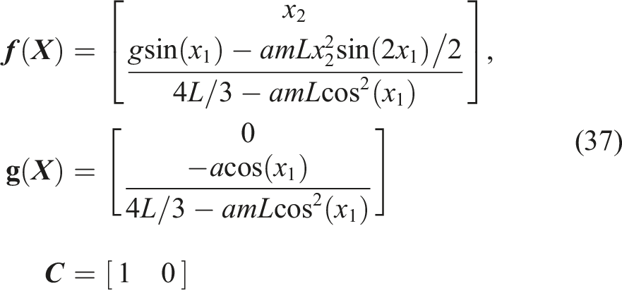
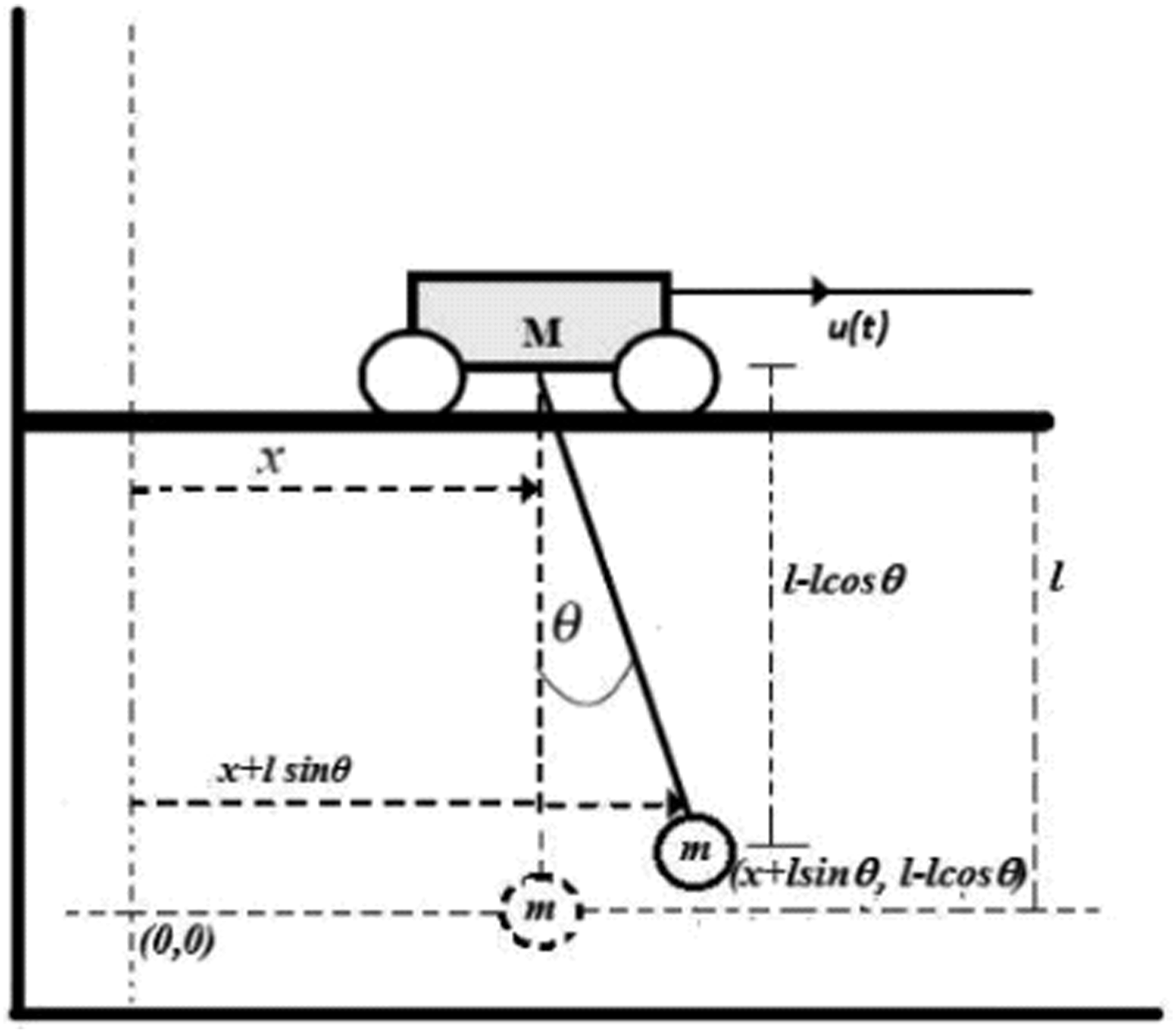
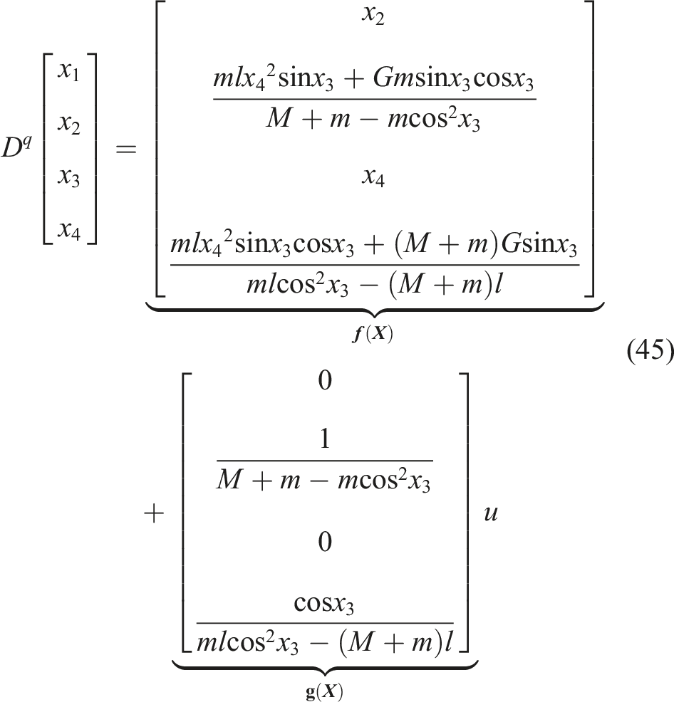
where pendulum angle ( $\theta$ ) from the vertical axis and angular velocity ( $D^q\theta$ ) are revealed by $x_1$ and $x_2$ , respectively, and $q=0.4$ . The gravity constant is shown by $g=9.8\hspace{0.17em}m/s^2$ . Pendulum mass is denoted by $m$ . $M$ and $L$ are the symbols for cart mass and pendulum length, respectively, and $a=1/(m+M)$ . The force utilized in the cart is $u=F=5\sin (5t)\hspace{0.17em}N$ . Parameters of the system are selected as $m=2\hspace{0.17em}\mathrm{k}\mathrm{g},\hspace{0.17em}M=8\hspace{0.17em}\mathrm{k}\mathrm{g}$ and $L=0.5\hspace{0.17em}m$ .

Figure 1.

Inverted pendulum on a cart.

Equation (36) can be rewritten as the following

$\{\begin{array}{c}{D}^q\mathit{X}(t)=\mathit{f}(\mathit{X})+\mathbf{g}(\mathit{X})u\\ \mathit{y}=\mathit{C}\mathit{X}\hspace{0.17em}\end{array}$

$\begin{array}{c}\mathit{f}(\mathit{X})=\left[\begin{array}{c}{x}_2\\ \frac{g\sin (x_1)-amL{x}_2^2\sin (2x_1)/2}{4L/3-amL{\cos }^2(x_1)}\end{array}\right],\hspace{0.17em}\mathbf{g}(\mathit{X})=\left[\begin{array}{c}0\\ \frac{-a\cos (x_1)}{4L/3-amL{\cos }^2(x_1)}\end{array}\right]\\ \mathit{C}=\left[\begin{array}{cc}1& 0\end{array}\right]\hspace{0.17em}\end{array}$

(37)

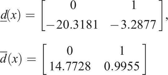
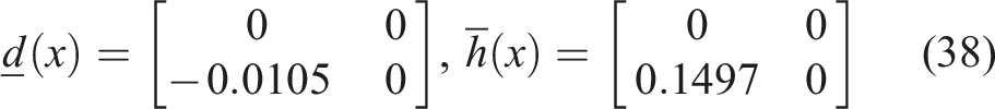
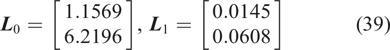
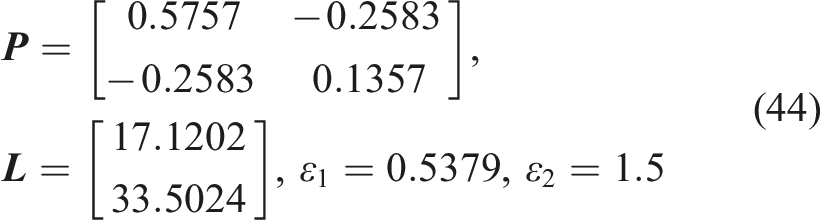
Applying our approach and carrying out the simulation, the values of $\left\{{\underset{\_}{\underset{\_}{d}}}_{ij},{\overline{d}}_{ij}\right\}$ and $\left\{{\underset{\_}{\underset{\_}{h}}}_{ij},{\overline{h}}_{ij}\right\}$ are found as

$\underset{\_}{\underset{\_}{d}}(x)=\left[\begin{array}{cc}0& 1\\ -20.3181& -3.2877\end{array}\right],\hspace{0.17em}\overline{d}(x)=\left[\begin{array}{cc}0& 1\\ 14.7728& 0.9955\end{array}\right]$

$\underset{\_}{\underset{\_}{d}}(x)=\left[\begin{array}{cc}0& 0\\ -0.0105\hspace{0.17em}& 0\end{array}\right],\hspace{0.17em}\overline{h}(x)=\left[\begin{array}{cc}0& 0\\ 0.1497& 0\end{array}\right]$

(38)

According to (38), the sets of ${\mathcal{V}}_{D_{n,n}}$ and ${\mathcal{V}}_{H_{n,n}}$ have $\alpha =2^2=4$ and $\beta =2^1=2$ vertices, respectively. By solving LMIs (19) and (20) (Case 3) using Yalmip toolbox and Mosek solver, it obtains

${\mathit{L}}_0=\left[\begin{array}{c}1.1569\\ 6.2196\end{array}\right],\hspace{0.17em}{\mathit{L}}_1=\left[\begin{array}{c}0.0145\\ 0.0608\end{array}\right]$

(39)

Using these two gains ( ${\mathit{L}}_0$ and ${\mathit{L}}_1$ ), asymptotic convergence of the estimation error toward zero is guaranteed. In order to determine the effectiveness of our method, it would be interesting to compare our approach with the one that is suggested in Lan et al. (2016). The nonlinear Lipschitz system is addressed below according to Lan et al. (2016)

$\{\begin{array}{c}{D}^q\mathit{x}(t)=\mathit{A}\mathit{x}(t)+\mathit{\Phi }(\mathit{x}(t),\mathit{u}(t))\\ \mathit{y}(t)=\mathit{C}\mathit{x}(t)\hspace{0.17em}\end{array}$

(40)

where $\mathit{x}\in R^n$ is the state vector, $\mathit{u}\in R^m$ is the input, $\mathit{y}\in R^p$ is the output, that is, the measurable output variables of the system, and $\mathit{A}\hspace{0.17em}\mathrm{a}\mathrm{n}\mathrm{d}\hspace{0.17em}\mathit{C}$ is the matrix with appropriate dimensions. The nonlinear function $\mathit{\Phi }(\mathit{x},\mathit{u}):R^n\to R^n$ is said to be locally Lipschitz in a region $\mathbb{D}$ including the origin with respect to $\mathit{x}$ , uniformly in $\mathit{u}$ , if for all ${\mathit{x}}_{\mathbf{1}},\hspace{0.17em}{\mathit{x}}_{\mathbf{2}}\in \mathbb{D}$ , there exists a constant γ > 0 satisfying

$\Vert \mathit{\Phi }({\mathit{x}}_{\mathbf{1}},{\mathit{u}}^{*})-\mathit{\Phi }({\mathit{x}}_{\mathbf{2}},{\mathit{u}}^{*})\Vert \le \gamma \Vert {\mathit{x}}_{\mathbf{1}}-{\mathit{x}}_{\mathbf{2}}\Vert$

(41)

The suggested observer is (Lan et al., 2016)

$\{\begin{array}{c}{D}^q\widehat{\mathit{x}}(t)=\mathit{A}\widehat{\mathit{x}}(t)+\mathit{\Phi }(\widehat{\mathit{x}}(t),\mathit{u}(t))+\mathit{L}(\mathit{y}(t)-\widehat{\mathit{y}}(t))\\ \widehat{\mathit{y}}(t)=\mathit{C}\widehat{\mathit{x}}(t)\hspace{0.17em}\end{array}$

(42)

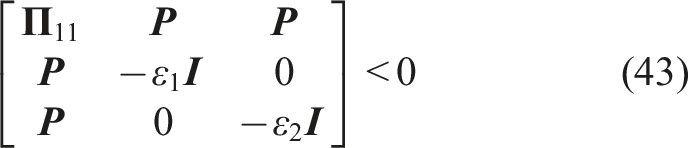
According to Lan et al. (2016), the observer error dynamic system asymptotically converges if there exist a symmetrical matrix $\mathit{P}\hspace{0.17em}>\hspace{0.17em}0$ and matrix $\mathit{Z}$ of appropriate dimensions together with real scalars ${\epsilon }_1\hspace{0.17em}>\hspace{0.17em}0,\hspace{0.17em}{\epsilon }_2\hspace{0.17em}>\hspace{0.17em}0$ such that

$\left[\begin{array}{ccc}{\mathbf{\Pi }}_{11}& \mathit{P}& \mathit{P}\\ \mathit{P}& -{\epsilon }_1\mathit{I}& 0\\ \mathit{P}& 0& -{\epsilon }_2\mathit{I}\end{array}\right]<0$

(43)

where ${\mathbf{\Pi }}_{11}=\mathit{P}\mathit{A}+{\mathit{A}}^{\mathit{T}}\mathit{P}-\mathit{Z}\mathit{C}-{\mathit{C}}^{\mathit{T}}{\mathit{Z}}^{\mathit{T}}+{\epsilon }_1\gamma \mathit{I}$ . Moreover, the observer gain can be chosen as $L={\mathit{P}}^{-\mathbf{1}}\mathit{Z}$ .

By considering the Lipschitz constant for this example as ( $\gamma =0.5$ ) and solving LMIs (43) using Yalmip toolbox and Mosek solver, it can obtain

$\mathit{P}=\left[\begin{array}{cc}0.5757& -0.2583\\ -0.2583& 0.1357\end{array}\right],\hspace{0.17em}\mathit{L}=\left[\begin{array}{c}17.1202\\ 33.5024\end{array}\right],\hspace{0.17em}{\epsilon }_1=0.5379,\hspace{0.17em}{\epsilon }_2=1.5$

(44)

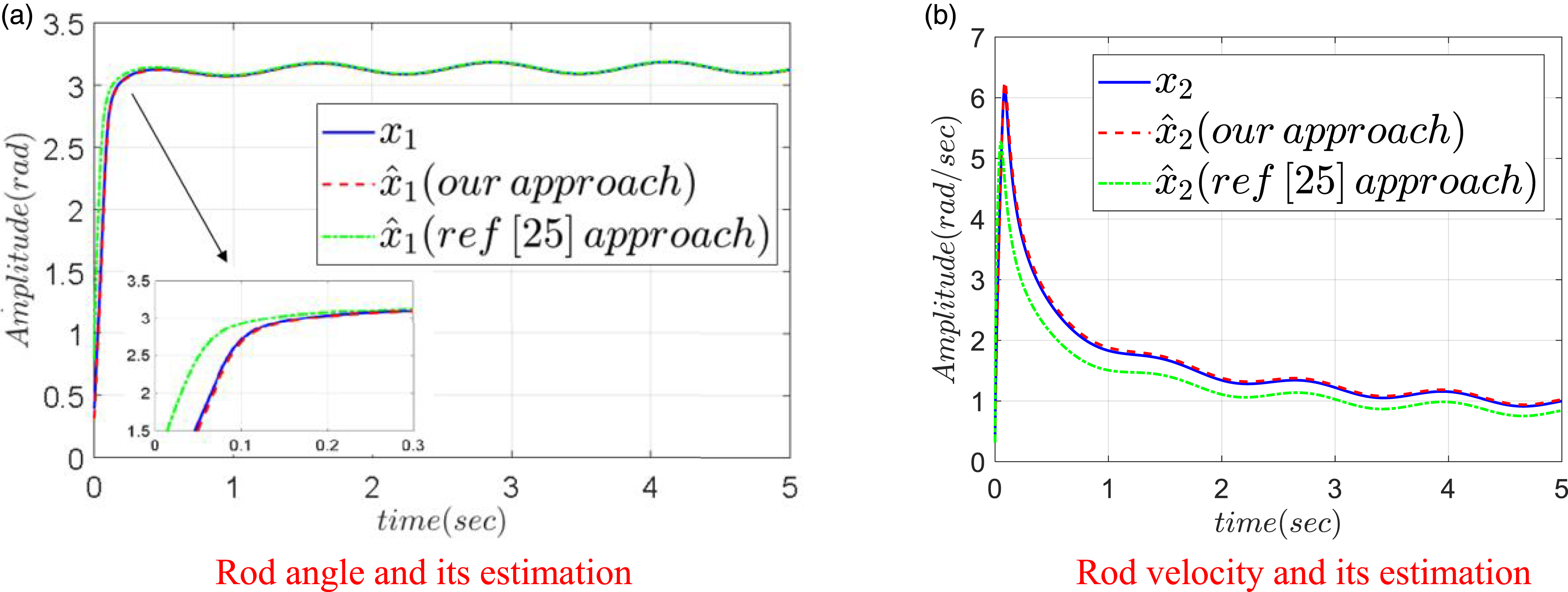
The comparison of the rod angle ( $\theta$ ) and the rod velocity ( $D^q\theta$ ) estimation and their actual values are illustrated in Figure 2(a) and (b), respectively, in the sense of our approach and the one in Lan et al. (2016). In this example, the initial conditions for the system and observer have been chosen as $\mathit{X}(0)=\left[\begin{array}{cc}\frac{\pi }{3}& \frac{\pi }{8}\end{array}\right]$ and $\widehat{\mathit{X}}(0)={\left[\begin{array}{cc}\frac{\pi }{4}& \frac{\pi }{10}\end{array}\right]}^T$ , respectively.

Figure 2.

(a) Rod angle and its estimation and (b) rod velocity and its estimation.

Example 2

As shown in Figure 3, the 2-D gantry crane is used to move heavy loads in factories, ships, etc.

Figure 3.

Schematic diagram of 2-D gantry crane.

The nonlinear FO state space representation of the 2-D gantry crane is given by (Pal Singh et al., 2017)

$D^q\left[\begin{array}{c}{x}_1\\ x_2\\ x_3\\ x_4\end{array}\right]=\underset{\mathit{f}(\mathit{X})}{\underbrace{\left[\begin{array}{c}\begin{array}{c}{x}_2\\ \frac{ml{x_4}^2\sin x_3+Gm\sin x_3\cos x_3}{M+m-m{\cos }^2{x}_3}\\ x_4\end{array}\\ \frac{ml{x_4}^2\sin x_3\cos x_3+(M+m)G\sin x_3}{ml{\cos }^2{x}_3-(M+m)l}\end{array}\right]}}+\underset{\mathbf{g}(\mathit{X})}{\underbrace{\left[\begin{array}{c}\begin{array}{c}0\\ \frac{1}{M+m-m{\cos }^2{x}_3}\\ 0\end{array}\\ \frac{\cos x_3}{ml{\cos }^2{x}_3-(M+m)l}\end{array}\right]}}u$

(45)

$\mathit{y}=\left[\begin{array}{cc}\begin{array}{cc}1& 0\end{array}& \begin{array}{cc}0& 0\end{array}\\ \begin{array}{cc}0& 0\end{array}& \begin{array}{cc}1& 0\end{array}\end{array}\right]\mathit{X}$

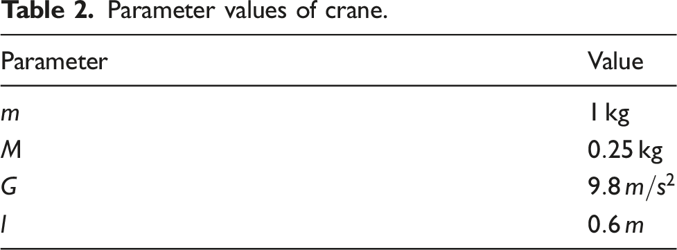
where $m$ and $M$ are load mass and trolley mass, respectively. $q=0.6$ , $l$ is cable length, and $u=10+10\sin (t)$ is the force applied to the system. $x_1(t)=x(t)$ and $x_3(t)=\theta (t)$ are the position of the trolley and tilt angle, respectively. Parameter values of the crane are given in Table 2.

Table 2.

Parameter values of crane.

Parameter	Value
$m$	$1\hspace{0.17em}\mathrm{k}\mathrm{g}$
$M$	$0.25\hspace{0.17em}\mathrm{k}\mathrm{g}$
$G$	$9.8\hspace{0.17em}m/s^2$
$l$	$0.6\hspace{0.17em}m$

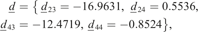
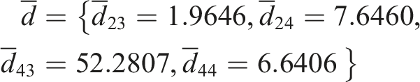
Here, the values of $\left\{{\underset{\_}{\underset{\_}{d}}}_{ij},{\overline{d}}_{ij}\right\}$ and $\left\{{\underset{\_}{\underset{\_}{m}}}_{ij},{\overline{m}}_{ij}\right\}$ are obtained as

$\underset{\_}{\underset{\_}{d}}=\left\{{\underset{\_}{\underset{\_}{d}}}_{23}=-16.9631,\hspace{0.17em}{\underset{\_}{\underset{\_}{d}}}_{24}=0.5536,{\underset{\_}{\underset{\_}{d}}}_{43}=-12.4719,{\underset{\_}{\underset{\_}{d}}}_{44}=-0.8524\right\},$

$\overline{d}=\left\{{\overline{d}}_{23}=1.9646,{\overline{d}}_{24}=7.6460,{\overline{d}}_{43}=52.2807,{\overline{d}}_{44}=6.6406\hspace{0.17em}\right\}$

${\underset{\_}{\underset{\_}{d}}}_{12}={\overline{d}}_{12}=1.0\hspace{0.17em},\hspace{0.17em}{\underset{\_}{\underset{\_}{d}}}_{34}={\overline{d}}_{34}=1.0$

$The\hspace{0.17em}remain\hspace{0.17em}elements\hspace{0.17em}of\hspace{0.17em}d\hspace{0.17em}are\hspace{0.17em}zero.$

$\underset{\_}{\underset{\_}{h}}=\left\{{\underset{\_}{\underset{\_}{h}}}_{23}=-4.4990,{\underset{\_}{\underset{\_}{h}}}_{43}=-2.2608\right\},$

$\overline{m}=\left\{{\overline{m}}_{23}=0.9291,{\overline{m}}_{43}=8.5364\right\}$

$The\hspace{0.17em}remain\hspace{0.17em}elements\hspace{0.17em}of\hspace{0.17em}m\hspace{0.17em}are\hspace{0.17em}zero.$

(46)

According to (46), the sets of ${\mathcal{V}}_{D_{n,n}}$ and ${\mathcal{V}}_{H_{n,n}}$ have $\alpha =2^4=16$ and $\beta =2^2=4$ vertices, respectively. Solving LMIs (18) using Yalmip toolbox and Mosek solver, it is found that

${\mathit{L}}_0=\left[\begin{array}{cc}\begin{array}{c}115.4\\ 9340.6\end{array}& \begin{array}{c}73.5\\ 5969\end{array}\\ \begin{array}{c}41.3\\ 6183.9\end{array}& \begin{array}{c}38\\ 5651.2\end{array}\end{array}\right],\hspace{0.17em}{\mathit{L}}_1=\left[\begin{array}{cc}\begin{array}{c}0.6189\\ 15.7863\end{array}& \begin{array}{c}0.0392\\ 5.5756\end{array}\\ \begin{array}{c}0.0392\\ 10.2935\end{array}& \begin{array}{c}0.5107\\ 5.4291\end{array}\end{array}\right]$

(47)

Simulation is done using Simulink with the FOMCON toolbox to solve the fractional system model, and it is run for 10 s. Initial conditions for the system and the observer are assumed as ${\mathit{X}}_0={(0,\hspace{0.17em}0,\hspace{0.17em}\frac{\pi }{8},\hspace{0.17em}0)}^T$ and ${\widehat{\mathit{X}}}_0={(1,\hspace{0.17em}\mathrm{2,0},\hspace{0.17em}2)}^T$ , respectively. The obtained results are shown in Figures 4–7.

Figure 4.

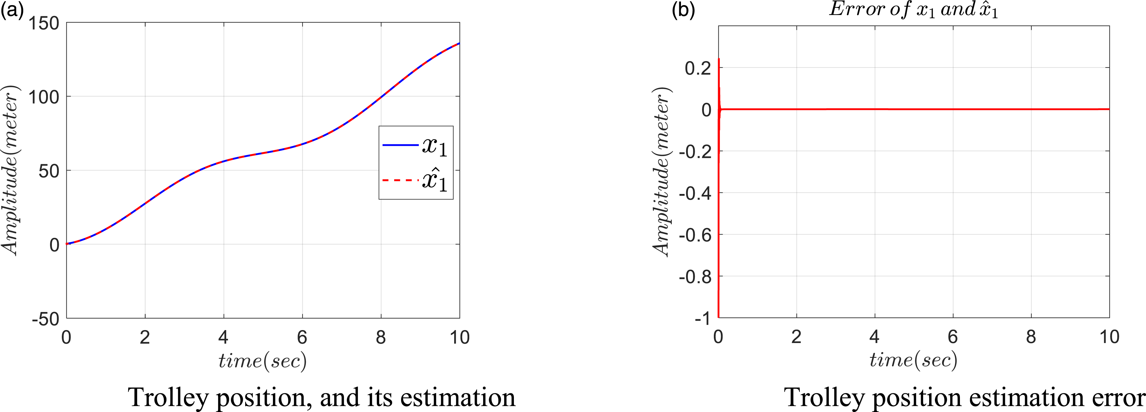
(a) Trolley position and its estimation and (b) trolley position estimation error.

Figure 5.

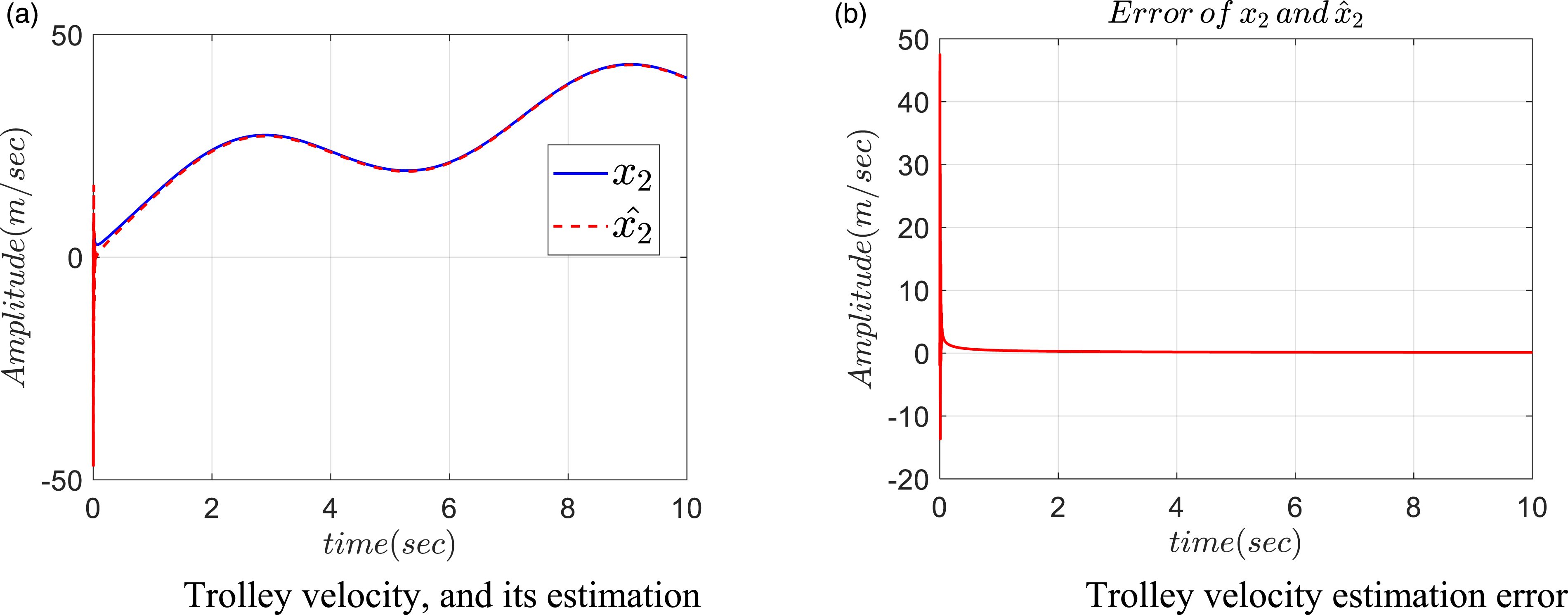
(a) Trolley velocity and its estimation and (b) trolley velocity estimation error.

Figure 6.

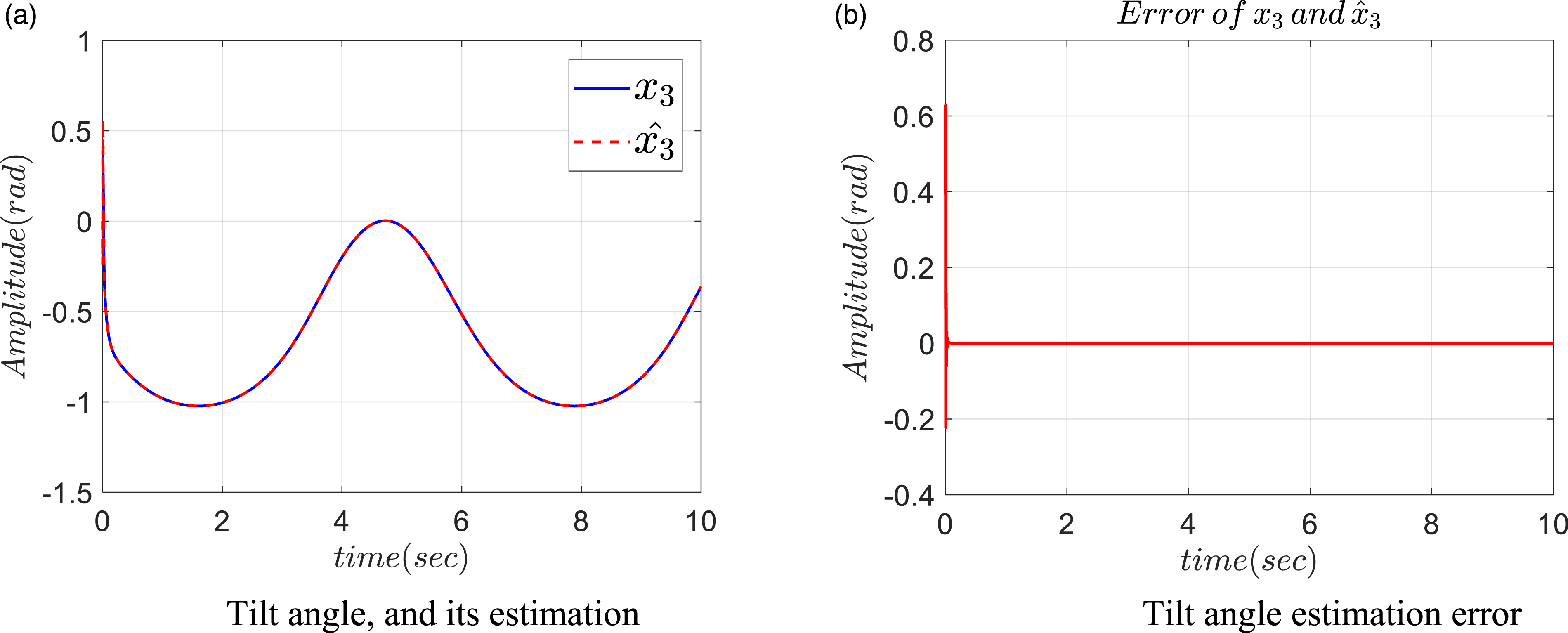
(a) Tilt angle and its estimation and (b) tilt angle estimation error.

Figure 7.

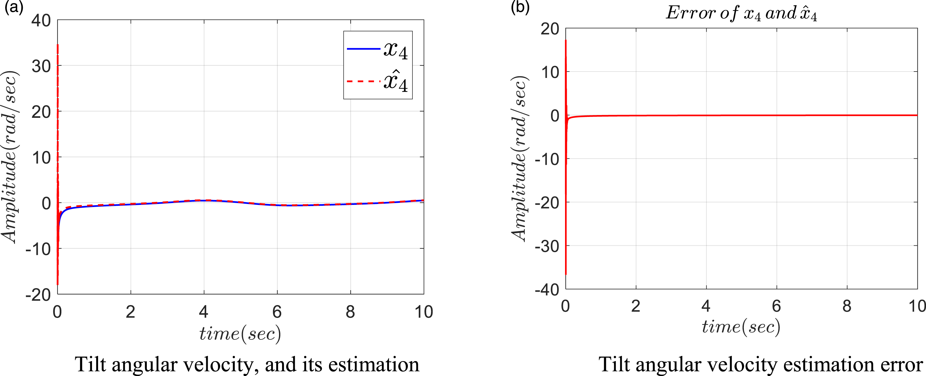
(a) Tilt angular velocity and its estimation and (b) tilt angular velocity estimation error.

Figure 4(a) displays the convergence results for the trolley position ( $x_1(t)$ ) and its estimation ( ${\widehat{x}}_1(t)$ ), in which the trolley position estimation error is shown in Figure 4(b). Figure 5(a) gives a plot of trolley velocity ( $x_2(t)$ ) and its estimation ( ${\widehat{x}}_2(t)$ ), and the trolley velocity estimation error is depicted in Figure 5(b). Looking at Figure 6(a), it is apparent that estimation of the state of tilt angle ( ${\widehat{x}}_3(t)$ ) converges to its actual value ( $x_3(t)$ ) in a reasonable manner, whereas this claim is illustrated in Figure 6(b). Noticing Figure 7(a), it can be noted that estimation of tilt angular velocity ( ${\widehat{x}}_4(t)$ ) can move toward its actual value ( $x_4(t)$ ) in less than 2 s. This is revealed in Figure 7(b) that the estimation error of tilt angular velocity is converged to zero.

Example 3

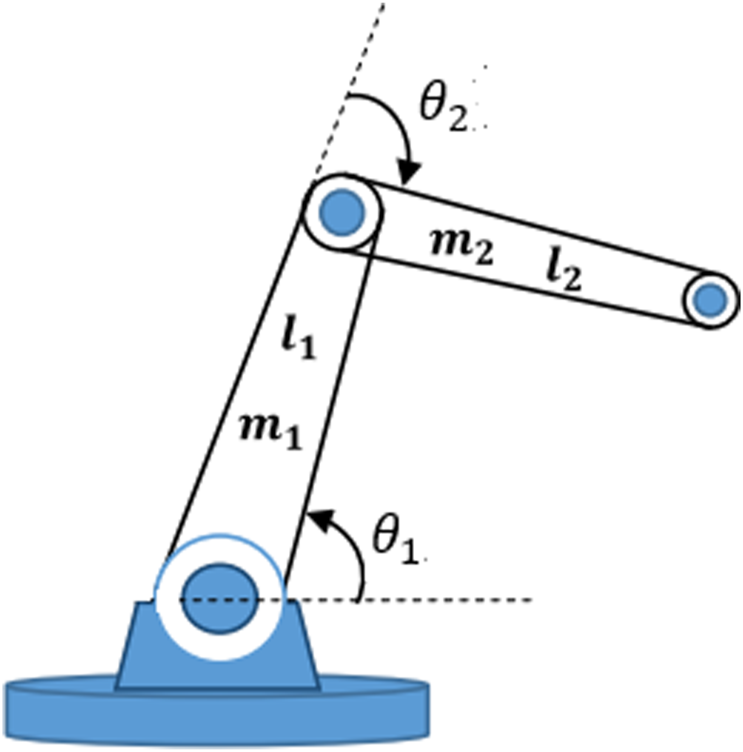
The final case study is a MIMO nonlinear system. A planar two-link robot manipulator model is considered, which is depicted in Figure 8. The joint angles can be displayed by vector $\mathit{\theta }={({\theta }_1,{\theta }_2)}^T$ , as the outputs and 2-input torque ( $\mathit{\tau }={({\tau }_1,{\tau }_2)}^T$ ), which are applied at the manipulator’s joints.

Figure 8.

Two-link robot manipulator.

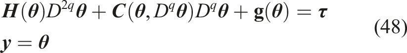
A nonlinear dynamic model of the robot manipulator based on the integer-order form has been introduced in Slotin and Weiping (1991). It can be written in MIMO fractional-order form as

$\mathit{H}(\mathit{\theta })D^{2q}\mathit{\theta }+\mathit{C}(\mathit{\theta },D^q\mathit{\theta })D^q\mathit{\theta }+\mathbf{g}(\mathit{\theta })=\mathit{\tau }\hspace{0.17em}\mathit{y}=\mathit{\theta }$

(48)

where $\mathit{H}(\mathit{\theta })$ is the $2\times 2$ symmetric positive definite inertia matrix of the manipulator, $\mathit{C}(\mathit{\theta },D^q\mathit{\theta })D^q\mathit{\theta }$ is the vector of centripetal and Coriolis torques, and $\mathbf{g}(\mathit{\theta })$ is the vector of gravitational torques. It is supposed that $\mathbf{g}(\mathit{\theta })\equiv \mathbf{0}$ , which implies the robot manipulator is in the horizontal plane.

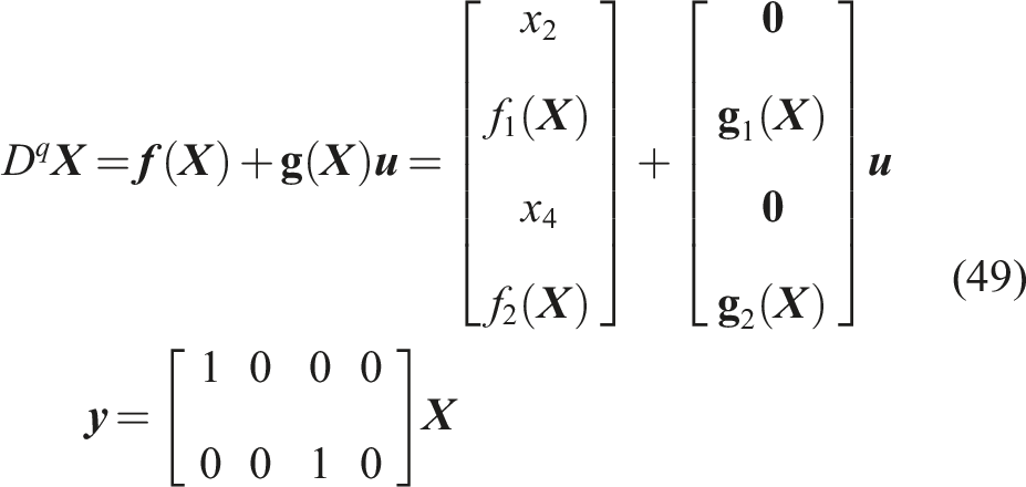
Suppose that $\mathit{X}={\left[x_1,x_2,x_3,x_4\right]}^T=\left[{\theta }_1,D^q{\theta }_1,{\theta }_2,D^q{\theta }_2\right]$ and $\mathit{\tau }=\mathit{u}={\left[u_1,u_2\right]}^T$ in which $u_1(t)=1$ , for $t\ge 0$ and $u_2(t)=2$ , for $t\ge 2$ , otherwise $\mathit{u}=\mathbf{0}$ . Equation (48) can be written in the state space form as

$D^q\mathit{X}=\mathit{f}(\mathit{X})+\mathbf{g}(\mathit{X})\mathit{u}=\left[\begin{array}{c}\begin{array}{c}{x}_2\\ f_1(\mathit{X})\end{array}\\ \begin{array}{c}{x}_4\\ f_2(\mathit{X})\end{array}\end{array}\right]+\left[\begin{array}{c}\begin{array}{c}\mathbf{0}\\ {\mathbf{g}}_1(\mathit{X})\end{array}\\ \begin{array}{c}\mathbf{0}\\ {\mathbf{g}}_2(\mathit{X})\end{array}\end{array}\right]\mathit{u}\hspace{0.17em}\mathit{y}=\left[\begin{array}{c}\begin{array}{cc}\begin{array}{cc}1& 0\end{array}& \begin{array}{cc}0& 0\end{array}\end{array}\\ \begin{array}{cc}\begin{array}{cc}0& 0\end{array}& \begin{array}{cc}1& 0\end{array}\end{array}\end{array}\right]\mathit{X}$

(49)

where $\left[f_1(\mathit{X}),f_2(\mathit{X})\right]=-{\mathit{H}(\mathit{\theta })}^{-1}\left[\mathit{C}(\mathit{\theta },D^q\mathit{\theta })D^q\mathit{\theta }\right]$ , $\left[{\mathrm{g}}_1(\mathit{X}),{\mathrm{g}}_2(\mathit{X})\right]=\left[{\mathrm{g}}_{11}(\mathit{X}),{\mathrm{g}}_{12}(\mathit{X});{\mathrm{g}}_{21}(\mathit{X}),{\mathrm{g}}_{22}(\mathit{X})\right]={\mathit{H}(\mathit{\theta })}^{-1}$ , and $q=0.5$ .

According to Slotin and Weiping (1991), $\mathit{H}(\mathit{\theta })$ and $\mathit{C}(\mathit{\theta },D^q\mathit{\theta })$ are defined as

$\mathit{H}(\mathit{\theta })=\left[\begin{array}{c}\begin{array}{cc}1.2\mathit{sin}{\theta }_2+2.0785\mathit{cos}{\theta }_2+3.34& 0.6\mathit{sin}{\theta }_2+1.0392\mathit{cos}{\theta }_2+0.97\end{array}\\ \begin{array}{cc}0.6\mathit{sin}{\theta }_2+1.0392\mathit{cos}{\theta }_2+0.97& 0.97\hspace{0.17em}\end{array}\end{array}\right]$

$\mathit{C}(\mathit{\theta },D^q\mathit{\theta })=\left[\begin{array}{c}\begin{array}{cc}0.6D^q{\theta }_2\mathit{cos}{\theta }_2-1.0392\mathit{sin}{\theta }_2& \hspace{0.17em}0.6(D^q{\theta }_1+D^q{\theta }_2)\mathit{cos}{\theta }_2-1.0392(D^q{\theta }_1+D^q{\theta }_2)\mathit{sin}{\theta }_2\end{array}\\ \begin{array}{cc}-0.6D^q{\theta }_1\mathit{cos}{\theta }_2+1.0392D^q{\theta }_1\mathit{sin}{\theta }_2\hspace{0.17em}& \hspace{0.17em}0.0\hspace{0.17em}\end{array}\end{array}\right]$

(50)

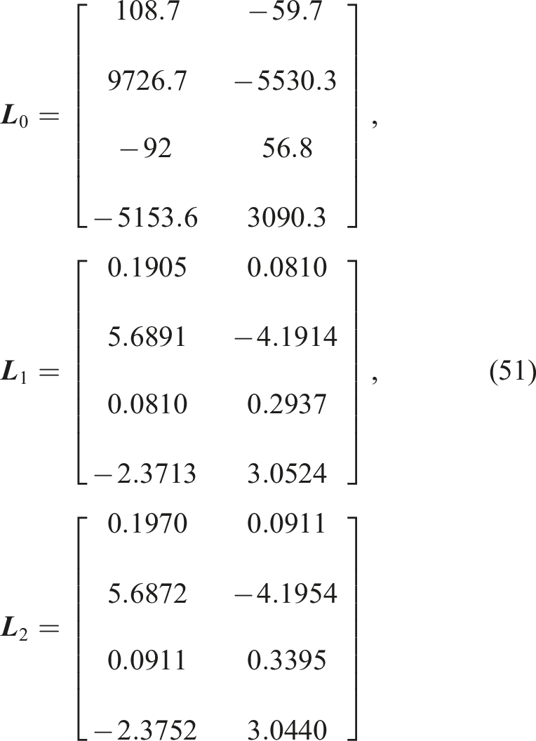
Now, by carrying out the simulation and finding the vertices of ${\mathcal{V}}_{D_{n,n}}$ and ${\mathcal{V}}_{H_{n,n}^k}(\hspace{0.17em}k=\mathrm{1,2})$ , LMIs (18) can be solved by Yalmip toolbox and Mosek solver. The gain vectors, that is, ${\mathit{L}}_0$ and ${\mathit{L}}_k,\hspace{0.17em}k=\mathrm{1,2}$ , can be obtained

${\mathit{L}}_0=\left[\begin{array}{cc}\begin{array}{c}108.7\\ 9726.7\end{array}& \begin{array}{c}-59.7\\ -5530.3\end{array}\\ \begin{array}{c}-92\\ -5153.6\end{array}& \begin{array}{c}56.8\\ 3090.3\end{array}\end{array}\right]\hspace{0.17em},\hspace{0.17em}{\mathit{L}}_1=\left[\begin{array}{cc}\begin{array}{c}0.1905\\ 5.6891\end{array}& \begin{array}{c}0.0810\\ -4.1914\end{array}\\ \begin{array}{c}0.0810\\ -2.3713\end{array}& \begin{array}{c}0.2937\\ 3.0524\end{array}\end{array}\right]\hspace{0.17em},\hspace{0.17em}{\mathit{L}}_2=\left[\begin{array}{cc}\begin{array}{c}0.1970\\ 5.6872\end{array}& \begin{array}{c}0.0911\\ -4.1954\end{array}\\ \begin{array}{c}0.0911\\ -2.3752\end{array}& \begin{array}{c}0.3395\\ 3.0440\end{array}\end{array}\right]$

(51)

Using the initial conditions ${\mathit{X}}_0={(0,\hspace{0.17em}0,\hspace{0.17em}0,\hspace{0.17em}0)}^{°\hspace{0.17em}T}$ and ${\widehat{\mathit{X}}}_0={(5,\hspace{0.17em}\mathrm{5,5},\hspace{0.17em}5)}^{°\hspace{0.17em}T}$ for the system and observer states, respectively, and the computed observer gain matrices ( ${\mathit{L}}_0\hspace{0.17em},\hspace{0.17em}{\mathit{L}}_1$ , and ${\mathit{L}}_2$ ), the Simulink simulation has been carried out with FOMCON toolbox for 10 s. The obtained results are presented in Figures 9–12.

Figure 9.

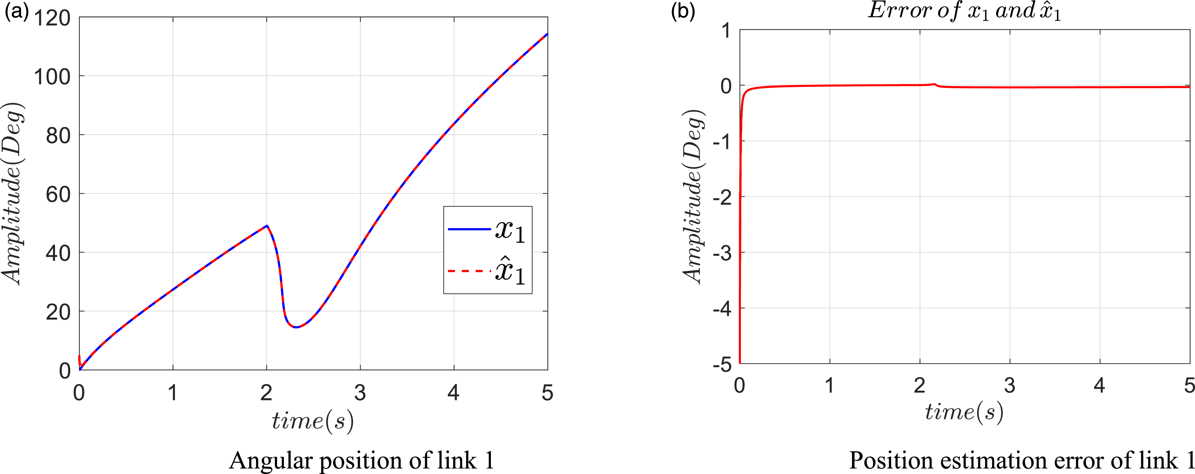
(a) Angular position of link 1 and (b) position estimation error of link 1.

Figure 10.

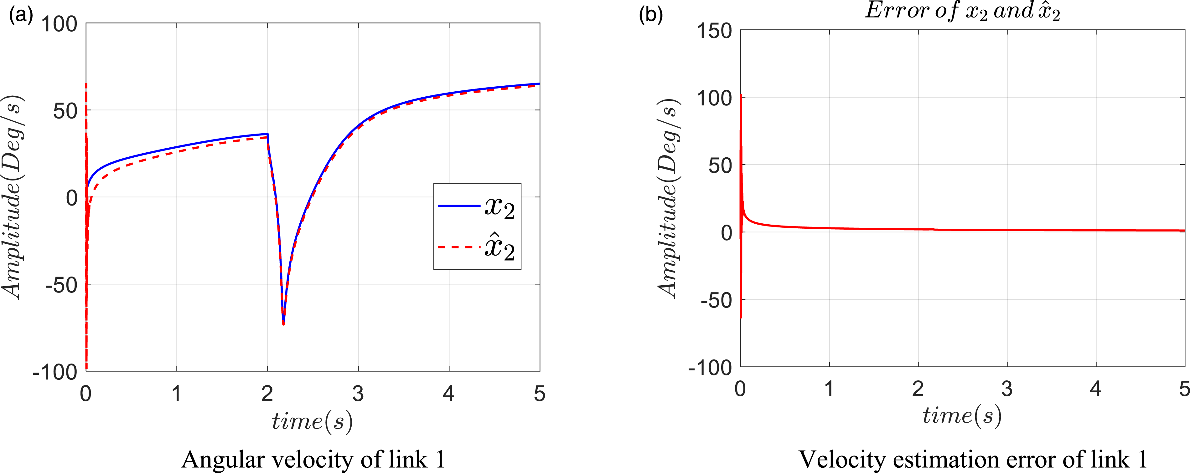
(a) Angular velocity of link 1 and (b) velocity estimation error of link 1.

Figure 11.

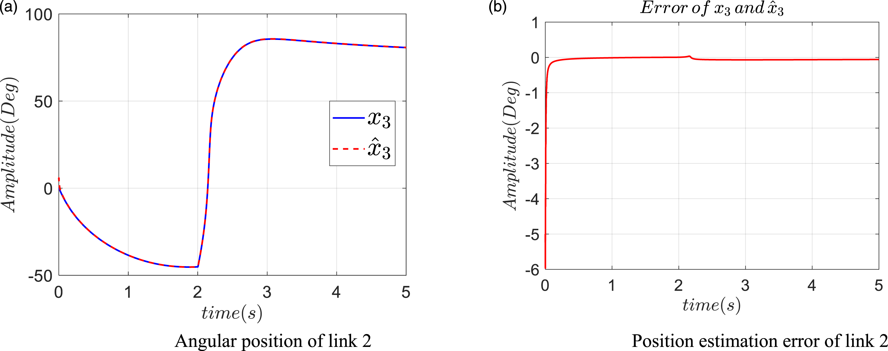
(a) Angular position of link 2 and (b) position estimation error of link 2.

Figure 12.

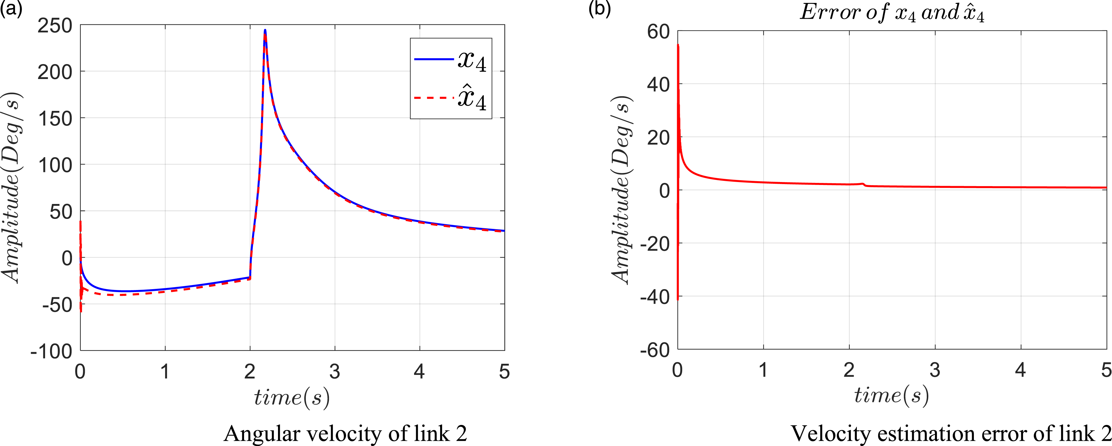
(a) Angular velocity of link 2 and (b) velocity estimation error of link 2.

Looking at the figures, it is apparent that all state estimation errors converge to zero.

6. Conclusion

In the current study, an observer has been designed for a general case of affine nonlinear FO MIMO systems. By DMVT-based approach, the proposed observer error’s dynamic is evolved as an LPV model. Using the convexity principle and solving a set of LMIs at vertices of a convex hull, gain matrices of the observer are designed. Furthermore, these observer gains are derived through the Lyapunov stability theory, that is, asymptotic convergence of the observation error toward zero is guaranteed. It must be noted that the proposed method can be applied to a general affine class of nonlinear integer-order dynamic systems. Numerical simulations have also been presented for three nonlinear FO systems to show the performance and efficacy of the proposed approach.