A unified approach for dynamic characteristic analysis of a standing-wave thermoacoustic engine with general impedance ends

Abstract

As promising devices for energy conversion, thermoacoustic engines (TAEs) are attracting more and more research attention with regard to renewable thermal energy application. For a TAE, the oscillation frequency is a critical parameter in its design and operation, which can only be estimated currently through an often tedious process using a shooting method or a numerical iteration method, and an analysis model with classical boundary conditions. In this context, this study seeks to establish a unified model for dynamic analysis of a one-dimensional (1D) standing-wave TAE with general impedance ends. First, the differential equations governing the thermoacoustic behavior of the TAE and its impedance boundary conditions are simultaneously solved using the Galerkin method and an improved Fourier series expansion method. Then, the characteristic distributions of oscillation frequency, sound pressure, and volume flow rate are obtained by solving a standard eigenvalue problem. Finally, the effects of engine length, stack length and position, and impedance ends on the dynamic behavior of the TAE’s thermoacoustic system are investigated and analyzed. The results show that engine length has a significantly negative correlation with the modal frequencies in different working gases, and stack position and stack length have a slight effect on the oscillation frequency of the TAE. The arbitrary variations in impedance boundary conditions can be simulated from the open end to the rigid wall and all intermediate cases. The proposed model can efficiently predict changes in dynamic parameters of 1-D TAEs with impedance ends in a unified pattern and can serve as a reliable analysis tool for further research on TAEs coupled with various energy harvesters.

Introduction

The recent years’ growing popularity of thermo-acoustic phenomena is built on their considerable potential in applications in the fields of energy conversion and refrigeration technology. Thermoacoustics is a major area of interest within both the fields of thermodynamics and acoustics, around which studies on thermoacoustic oscillation phenomena have been conducted in full swing. According to the different directions of energy transformation, thermoacoustic devices are usually categorized into thermoacoustic engines (TAEs) and thermoacoustic refrigerators. And TAEs can be further divided into standing-wave TAEs and traveling-wave TAEs based on the difference between oscillating sound pressure and velocity phase. A standing-wave TAE has the advantages of high sound pressure amplitude and high power density compared with a traveling-wave TAE, while it has the benefits of no moving parts, an elementary structure, a long service life, and environmental friendliness, compared with other types of heat engines. Therefore, standing-wave TAEs have enormous potential for further development, which results in considerable research efforts.

The thermoacoustic effect was first qualitatively described by Rayleigh (1878), who found the important phase relationship between the gas movement and ambient temperature for preserving acoustic oscillation around 130 years ago. Rott (1969) proposed a quantitative description of the thermoacoustic effect, and then, between 1972 and 1983 (Rott, 1972, 1975, 1980; Rott and Zouzoulas, 1976; 1983), further investigated the “Thermally Driven Acoustic Oscillations” in terms of stability limit, second-order heat flux, variable cross-section, etc. According to Rott’s summary (Swift et al., 1985; Swift, 1992, 2007, 2017; Swift and Kerlian, 1993, Swift and Spoor, 1999), simplified the governing equations in thermoacoustics under some assumptions and prepared DeltaEC (Design Environment for Low-amplitude Thermoacoustic Energy Conversion), the prominent software for TAE simulation analysis. Based on their work, an increasing research interest has been aroused in thermoacoustic systems.

There is a growing body of literature that recognizes the importance of the onset behavior of a standing-wave thermoacoustic engine. Tu et al. (2003) used the network theory to calculate the oscillation frequency of thermoacoustic system, and the theoretical results were in good agreement with those observed in experiments. Sugimoto and Yoshida (2007) and Sugimoto and Minamigawa (2019) established the theory of thermoacoustic oscillation in the closed tubes and derived the frequency equation from the boundary conditions at both ends of the tube. Furthermore, Sugimoto analyzed the stability of thermoacoustic oscillations and found the nonlinear phenomenon of pressure distribution in experiments. Guedra et al. (2010, 2011, 2014) proposed a thermoacoustic core transfer matrix method for the prediction of oscillation behavior, which avoids some assumptions, but the results still have relatively well precision. Limin et al. (2012) and Qiu et al. (2013) used the circuit network analogy to predict the engine onset temperature. On this basis, the influence of the porosity of stack on the onset temperature was explored experimentally. Chen and Jin (1999) and Chen et al. (2002) conducted the experiments to examine the onset and decay characteristics of thermoacoustic engines. The onset temperature of the hot source and frequency are two key variables that are essential to the onset characteristics. Sun et al. (2014) used the thermodynamic analysis to establish a simplified physical model of a standing-wave thermoacoustic engine in the time domain and used the model to calculate the sound pressure amplitude and spectral characteristics during the oscillation process. Boroujerdi and Ziabasharhagh (2016) used the wave propagation method to determine the oscillation frequency and onset temperature of a standing-wave TAE as eigenvalues of the fluctuation problem. In their study, the physical meaning of the wave propagation method was clear, but its theoretical derivations were slightly complicated, and the solution was time-consuming due to the iterations of large matrices.

Alternately, as computer technology advances, the finite element method (FEM) is gradually being implemented in the field of thermoacoustics. Nonetheless, the FEM method is essentially a meshing of the solution domain, and in some cases, mesh encryption is required. The analytical solution permits the parameterization of key properties, such as boundary conditions and geometry when modeling the object of the study. A quick prediction of the dynamical properties can be obtained by modifying the corresponding parameters, and therefore, an analytical method is urgently needed in the thermoacoustic. This method represents one of the most general theoretical modeling results for the swift and effective solution of the dynamical properties of thermoacoustic engines with arbitrary boundary conditions. Therefore, it is necessary to propose an analytical method for efficiently resolving thermoacoustic characterization issues.

In addition to the oscillational characteristics of thermoacoustic engine, the performance of the engine is also the focus of research attention, which is affected by various factors such as plate stack position, plate stack length, working gas type, and inflation pressure. To determine the effects of different working gases on the thermoacoustic behavior, Kalra et al. (2015) used the DeltaEC software to calculate the effects of engine structural parameters (such as engine length and plate stack length) and working gas types (Helium, Argon, Nitrogen, Carbon dioxide, Helium–Argon mixture, etc.) on the oscillation frequency, onset temperature, pressure amplitude, sound power, and efficiency of the thermoacoustic system. In addition, the engine performance is also influenced by its boundary conditions, and with the continuous progress of thermoacoustic technology, the connection of thermoacoustic engines with transducers provides the possibility of further utilization of thermoacoustic energy. Nowak et al. (2014) developed a thermoacoustic engine model with one open end and one closed end using analytical solution and numerical method and compared the results with those from simulation software to verify the model reliability. Based on this, Chen et al. (2018) established a boundary condition with one closed end and one end replaced by an endplate and investigated the effect of the endplate parameters on the performance of thermoacoustic engine. Nouh et al. (2013, 2014) investigated the effect of dynamic amplifiers on the performance of thermoacoustic engine with a piezoelectric transducer connected at one end, and the results showed the output efficiency of the engine could be improved by selecting the appropriate dynamic amplifier parameters.

The basic difference between a thermoacoustic heat engine and other heat engines is the way that sound wave propagates. The stack of thermoacoustic heat engines is placed in the resonant tube, and the propagation of its sound field depends on the constraints of the sound field of the whole thermoacoustic heat engine. It is becoming extremely difficult to ignore the existence of arbitrary boundaries of the sound field. The boundary conditions of sound field determine the sound field distribution, and the sound field distribution affects the coupling of fluid oscillation and temperature oscillation, which in turn affects the dynamic behavior of the thermoacoustic heat engine. Therefore, it is extremely necessary to propose a method that can uniformly solve the dynamic behavior of thermoacoustic heat engines with arbitrary impedance boundaries.

It is widely accepted that the Fourier series is used extensively in structural and acoustic modeling. However, the complexity of the thermoacoustic equations, such as viscous resistance and thermal relaxation, makes it difficult to solve them; consequently, no similar method has been adopted in the thermoacoustic field previously. This paper presents a solution for the dynamic characteristics of thermoacoustic engines with arbitrary boundary conditions, against the backdrop of increasingly complex boundary conditions and difficult control equations. This method is more effective than others for determining the structural parameters of thermoacoustic engines. The application of the extended Fourier series method to the thermoacoustic field permits the rapid generation of thermoacoustic characteristics under general impedance boundary conditions, overcoming the limitations of the prior method for the advancement of thermoacoustics. It also represents a novel mathematical application of the expanded Fourier series method.

As mentioned above, this study aims to expand a modified Fourier series to develop a model that can uniformly describe the oscillating frequency and dynamic behavior of a 1-D standing-wave TAE with general impedance ends. The remainder of this study is organized as follows. In Section 2, a model of the TAE is developed, and the Helmholtz equation for modeling sound pressure is formulated after the functional relationship between the oscillating frequency, the sound pressure and other parameters of the TAE under a given temperature difference is determined using the modified Fourier series. In Section 3, the accuracy of the proposed model is verified, based on which the effects of engine length, stack length, stack position, and the arbitrary boundary conditions at the onset frequency with the four working gases (i.e., H₂, He, N₂, and Ar) on the TAE are investigated, and the effects of the aforementioned factors on the modal distributions of sound pressure and volume flow rate are studied with H₂. And Section 4 concludes this study as the end.

Theoretical modeling

Model of a standing-wave thermoacoustic engine

As illustrated in Figure 1, the thermoacoustic engine includes the following main parts: hot buffer, stack, and resonator tube. The engine is considered as a cylindrical cavity with a radius of r₀ throughout. The left position of the stack of length (x _r -x_l) is fixed to x_l. The thick plate stack is 2l, providing a rectangular channel with a width of 2y₀ for working gas oscillation. The temperature at these two ends of the stack is high-temperature T _h and low-temperature T _c , respectively, and a linear temperature difference is established along with the plate stack due to the thermal conductivity of the solid material. When the temperature of the hot end rises continuously, making the temperature gradient at the stack the same as the onset temperature difference, thermoacoustic oscillations occur. At both ends of the thermoacoustic engine are arbitrary impedance boundaries with an impedance coefficient of Z₀ and Z_L, respectively. For the investigation of the thermoacoustic engine, its internal acoustic field serves as the research object in this paper. The linear thermoacoustic theory summarizes the effect of the solid domain and temperature field on the fluid as the temperature gradient coefficient and the thermal viscosity function. The procedure for modeling the internal flow field of a thermoacoustic engine is as follows.

Figure 1.

Schematic illustration of a typical standing-wave thermoacoustic engine with general impedance ends.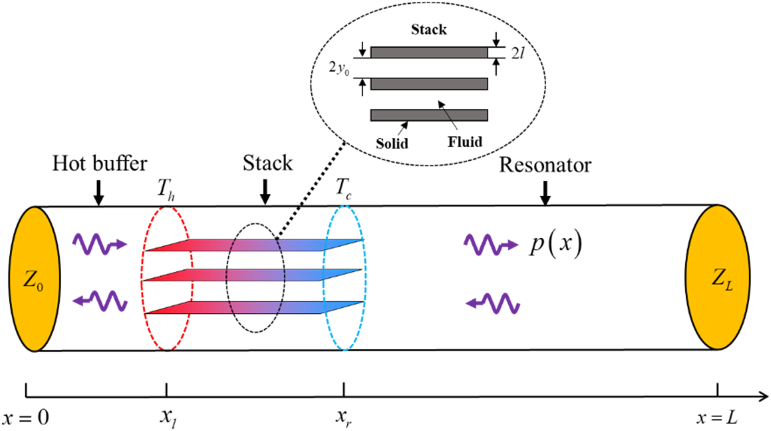

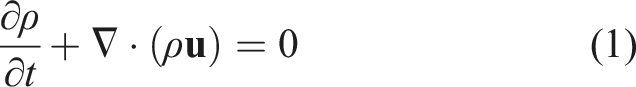
The continuity equation is written as

$\frac{\partial \rho }{\partial t}+\nabla \cdot \left(\rho \mathbf{u}\right)=0$

(1)

where ρ and $\mathbf{u}$ are the density and velocity of the fluid, respectively. $\nabla$ is the Vector differential operator and it can be written as $\nabla =\frac{\partial }{\partial x}+\frac{\partial }{\partial y}+\frac{\partial }{\partial z}$ .

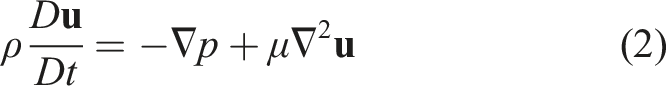
The momentum equation is

$\rho \frac{D\mathbf{u}}{Dt}=-\nabla p+\mu {\nabla }^2\mathbf{u}$

(2)

where p and μ are the pressure and dynamic viscosity of the fluid, ${\nabla }^2$ is the Laplace operator, it means ${\nabla }^2=\frac{{\partial }^2}{\partial x^2}+\frac{{\partial }^2}{\partial y^2}+\frac{{\partial }^2}{\partial z^2}$ , and $\frac{D\mathbf{u}}{Dt}=\frac{\partial \mathbf{u}}{\partial t}+\left(\mathbf{u}\cdot \nabla \right)\mathbf{u}$ .

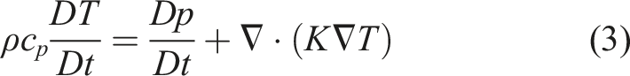
The energy equation is

$\rho c_p\frac{DT}{Dt}=\frac{Dp}{Dt}+\nabla \cdot \left(K\nabla T\right)$

(3)

where c_p, K, and T are the isobaric specific heat, thermal conductivity, and temperature of the fluid.

The state equation of gas is

$p=\rho RT$

(4)

where R is the gas constant.

By the Rott’s acoustic approximation, several significant physical quantities are considered as the summation of average and fluctuating quantities, namely,

$p\left(x,y,z,t\right)=p_m+\mathrm{R}\mathrm{e}\left[p_1\left(x\right)e^{i\omega t}\right]$

(5)

$u\left(x,y,z,t\right)=\mathrm{R}\mathrm{e}\left[u_1\left(x\right)e^{i\omega t}\right]$

(6)

$T\left(x,y,z,t\right)=T_m\left(x\right)+\mathrm{R}\mathrm{e}\left[T_1\left(x\right)e^{i\omega t}\right]$

(7)

where the subscripts m and 1 represent the average and fluctuating values of the physical quantities, Re is the real part of the physical quantities, i is the imaginary unit, and ω is the oscillating frequency, which is related to the frequency f as ω = 2πf.

Rott’s linear acoustic theory suggests that sound waves propagate only along the x-axis, so the average value of the physical quantities in equations (5)–(7) is only related to the x. He also considers that the average pressure p_m, that is, the charging pressure, is not related to all coordinates, and the average velocity u_m is zero.

Substituting equations (5)–(7) into equations (1)–(4), neglecting the second-order small terms, and integrating the x component of the velocity u₁ over the cross-section, the governing thermoacoustic control equation is obtained

$d{p}_1=\frac{-i\omega {\rho }_{m}dx}{S\left(1-f_v\right)}{U}_1$

(8)

$d{U}_1=\frac{-i\omega Sdx}{\gamma p_m}\left[1+\left(\gamma -1\right)f_k\right]p_1+\frac{f_k-f_v}{\left(1-f_v\right)\left(1-\mathrm{Pr}\right)}\frac{d{T}_m}{T_m}{U}_1$

(9)

where f _k and f _v are thermal-viscous functions related to the channel structure, S is the section area of the channel, U₁ is the volume flow velocity of the fluids, and Pr is the Prandtl number.

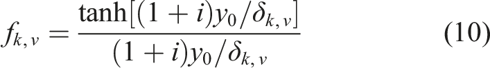
For the parallel plate pipes, the thermal-viscous function is

$f_{k,v}=\frac{\tanh \left[\left(1+i\right)y_0/{\delta }_{k,v}\right]}{\left(1+i\right)y_0/{\delta }_{k,v}}$

(10)

where y₀ is half of the plate spacing and δ_k and δ_v are thermal and viscous penetration depth, they can be written as ${\delta }_k=\sqrt{\frac{2K}{\omega {\rho }_m{c}_p}}$ and ${\delta }_v=\sqrt{\frac{2\mu }{\omega {\rho }_m}}$ , respectively.

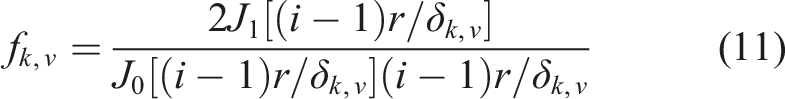
For a circular pipe, the thermal-viscous function is

$f_{k,v}=\frac{2J_1\left[\left(i-1\right)r/{\delta }_{k,v}\right]}{J_0\left[\left(i-1\right)r/{\delta }_{k,v}\right]\left(i-1\right)r/{\delta }_{k,v}}$

(11)

in which J is the Bessel function and r is the hydraulic radius.

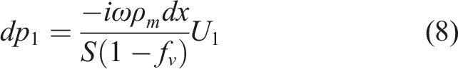
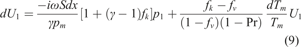
From equation (8), it can be seen that the movement of the gas causes a local pressure increase in the gas, leading to the generation of a pressure gradient dp₁. Similarly, from equation (9), it can be deduced that the gradient of the volume flow rate dU₁ of the gas is generated by two components: the pressure p₁ and the volume flow rate U₁ along the temperature gradient dT_m.

For the ease of solution, one can simplify the thermoacoustic governing equations (8) and (9) as shown below

$\frac{d{p}_1}{dx}=-\omega \alpha U_1$

(12)

$\frac{d{U}_1}{dx}=-\omega \beta p_1+\tau U_1$

(13)

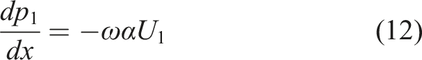
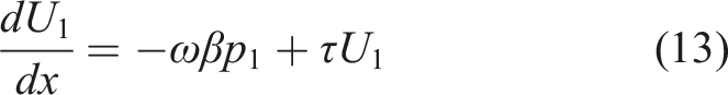
The coefficients are defined as follows

$\alpha =\frac{i{\rho }_m}{S\left(1-f_v\right)}$

(14)

$\beta =\frac{iS\left[1+\left(\gamma -1\right)f_k\right]}{\gamma p_m}$

(15)

$\tau =\frac{f_k-f_v}{\left(1-f_v\right)\left(1-\mathrm{Pr}\right)T_m}\frac{d{T}_m}{dx}$

(16)

where α, β, and τ are the coefficients, which were introduced to simplify the representation and to make the final thermoacoustic equation more concise and has no specific physical meaning.

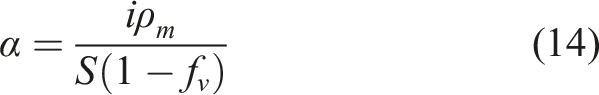
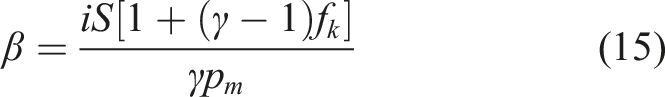
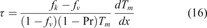
It is generally assumed that the average temperatures of the hot buffer, stack, and resonator are T_h, (T_h + T_c)/2, and T_c, respectively, so that the average density ρ_m inside the three regions do not change with the coordinate x. Hence, the coefficients α and β also do not change with x inside the three regions, but the coefficient τ exists only in the stack region and is zero in the other two leftover regions.

Combining equations (12) and (13), the Helmholtz equation for p₁ is obtained

$\frac{d^2{p}_1}{d{x}^2}-\tau \frac{d{p}_1}{dx}-{\omega }^2\alpha \beta p_1=0$

(17)

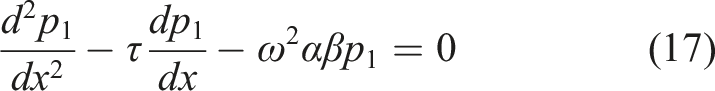
As can be seen from the above equation, if the thermal-viscous function is ignored, equation (17) degenerates into a classical wave equation $\frac{d^2{p}_1}{d{x}^2}+{\mathrm{\Omega }}^2{p}_1=0$ , where Ω is the wavenumber.

General impedance boundary conditions

As already mentioned in the previous introduction, for the solution of the thermoacoustic core governing equations, many methods such as wave propagation method, shooting method, and network analogy method have been proposed, but there is not a more comprehensive and systematic solution process for the coupling between the thermoacoustic equations and the boundary conditions. Inspired by the previous work by Du et al. (2011), this study further extends a modified Fourier series to reconstruct the thermoacoustic governing equations.

The classical boundary conditions in acoustics include rigid wall boundary conditions, soft boundary conditions, and impedance boundary conditions. This impedance is defined as the complex ratio between the sound pressure at the surface and the air velocity normal to the surface just outside the surface. In either case, a low acoustic impedance wall can be described as a “soft” wall, while a large impedance wall can be described as a “hard” wall. Hence, the arbitrary variations in impedance boundary conditions can be simulated from the open end to the rigid wall and all intermediate cases.

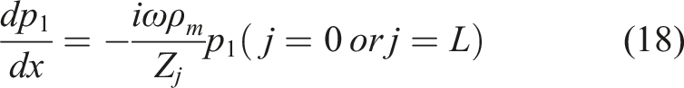
This paper uses the boundary impedance to portray the boundaries of the engine. In the complex value of the boundary impedance Z₀ and Z_L, the real part of the boundary impedance results in the dissipation of acoustic energy, and the imaginary part represents the elasticity, which is used to change the acoustic phase. The relationship between the sound pressure p₁ and the boundary impedance is fulfilled as

$\frac{d{p}_1}{dx}=-\frac{i\omega {\rho }_m}{Z_j}{p}_1\left(j=0\hspace{0.17em}or\hspace{0.17em}j=L\right)$

(18)

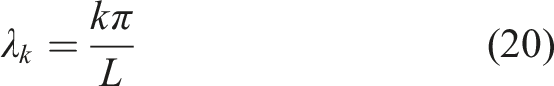
Generally, for an arbitrary periodic function, it can be expressed as a combination of sine and cosine. However, for the practical thermoacoustic problem in this paper, the sound pressure function p₁(x) is an arbitrary function defined on a finite range [0, L]. Since it is not periodic, and such a function can be expanded to the half-range Fourier series mentioned by Gu (2012). Mathematically, expanding p₁(x), $x\in \left[0,L\right]$ , into a Fourier cosine series is equivalent to viewing it as part of a periodic function which is simply p₁(x) over [-L, L]. Hence, the pressure can be written as

$p_1\left(x\right)={\displaystyle \sum }_{k=0}^{\infty }{a}_k\cos \left({\lambda }_{k}x\right)$

(19)

${\lambda }_k=\frac{k\pi }{L}$

(20)

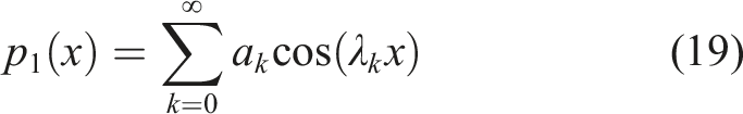
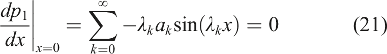
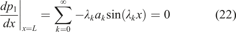
Combining equations (18) and (19), it can be seen that if the standard Fourier series is used to expand the sound pressure distribution, the first-order derivative of the sound pressure is zero at both boundaries, as shown in equations (21) and (22), making it impossible to relate the impedance boundary conditions to the sound pressure.

${\frac{d{p}_1}{dx}|}_{x=0}={\displaystyle \sum }_{k=0}^{\infty }-{\lambda }_k{a}_k\sin \left({\lambda }_{k}x\right)=0$

(21)

${\frac{d{p}_1}{dx}|}_{x=L}={\displaystyle \sum }_{k=0}^{\infty }-{\lambda }_k{a}_k\sin \left({\lambda }_{k}x\right)=0$

(22)

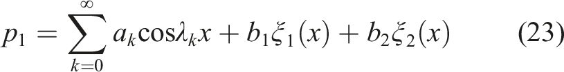
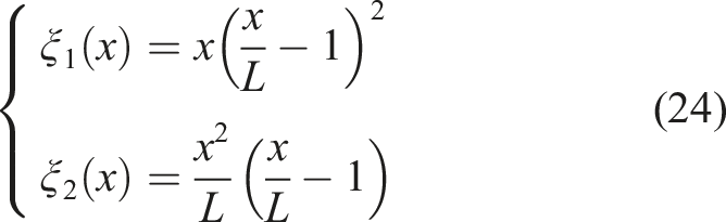
To overcome the issue of discontinuity of such sound pressure derivative at the boundary, the boundary-smoothed complementary function is introduced in this work, and the Fourier series expansion method after the introduction of the complementary function is called the modified Fourier series approach.

The sound pressure field function expanded by a modified Fourier series method can be written as

$p_1={\displaystyle \sum }_{k=0}^{\infty }{a}_k\cos {\lambda }_{k}x+b_1{\xi }_1\left(x\right)+b_2{\xi }_2\left(x\right)$

(23)

where ξ₁(x) and ξ₂(x) are the boundary-smoothed complementary function and b₁ and b₂ is the coefficient corresponding to the supplementary function. The complementary function can be any set of functions that can solve the problem of the boundary discontinuities of the first two derivatives of the sound pressure function, one example is given here

$\{\begin{array}{l}{\xi }_1\left(x\right)=x{\left(\frac{x}{L}-1\right)}^2\\ {\xi }_2\left(x\right)=\frac{x^2}{L}\left(\frac{x}{L}-1\right)\end{array}$

(24)

It’s easy to verify that

${\left[\begin{array}{cc}{\xi }_1\left(x\right)& {\xi }_2\left(x\right)\\ {\xi }_1^{\prime }\left(x\right)& {\xi }_2^{\prime }\left(x\right)\end{array}\right]|}_{x=0}=\left[\begin{array}{cc}0& 0\\ 1& 0\end{array}\right]$

(25)

${\left[\begin{array}{cc}{\xi }_1\left(x\right)& {\xi }_2\left(x\right)\\ {\xi }_1^{\prime }\left(x\right)& {\xi }_2^{\prime }\left(x\right)\end{array}\right]|}_{x=L}=\left[\begin{array}{cc}0& 0\\ 0& 1\end{array}\right]$

(26)

Substituting equation (23) into equation (18), one can obtain

${\frac{d{p}_1}{dx}|}_{x=0}=b_1{\xi }_1^{\prime }\left(0\right)+b_2{\xi }_2^{\prime }\left(0\right)=\frac{-i\omega {\rho }_m}{Z_0}{p}_1\left(0\right)=\frac{-i\omega {\rho }_m}{Z_0}{\displaystyle \sum }_{k=0}^{\infty }{a}_k=b_1$

(27)

${\frac{d{p}_1}{dx}|}_{x=L}=b_1{\xi }_1^{\prime }\left(L\right)+b_2{\xi }_2^{\prime }\left(L\right)=\frac{-i\omega {\rho }_m}{Z_L}{p}_1\left(L\right)=\frac{-i\omega {\rho }_m}{Z_L}{\displaystyle \sum }_{k=0}^{\infty }{\left(-1\right)}^k{a}_k=b_2$

(28)

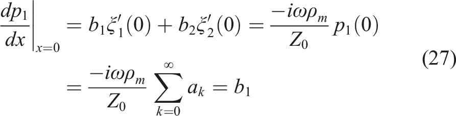
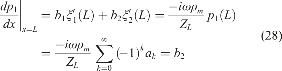
Equations (27) and (28) can be further converted into a matrix form, namely,

$\mathbf{B}=\omega \mathbf{Z}\mathbf{A}$

(29)

in which,

$\mathbf{A}=\left[\begin{array}{c}{a}_0\\ a_1\\ ...\\ a_k\end{array}\right]$

(30)

$\mathbf{B}=\left[\begin{array}{c}{b}_1\\ b_2\end{array}\right]$

(31)

$\mathbf{Z}=-i{\rho }_m\left[\begin{array}{cccc}\frac{1}{Z_0}& \frac{1}{Z_0}& ...& \frac{1}{Z_0}\\ \frac{1}{Z_L}& \frac{-1}{Z_L}& ...& \frac{{\left(-1\right)}^k}{Z_L}\end{array}\right]$

(32)

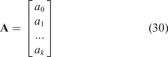
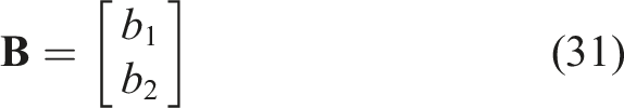
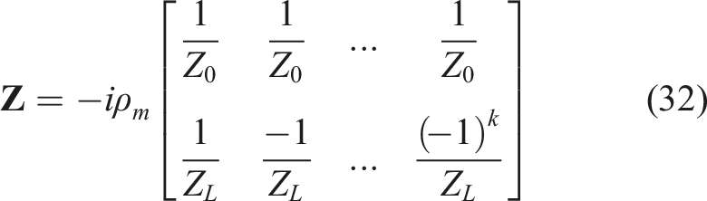
By using equation (29), the arbitrary impedance boundary is associated with the amplitude of sound pressure, and a unified representation of sound field and impedance boundary is then established.

Solution procedure of thermoacoustic engine dynamics

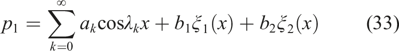
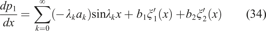
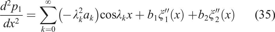
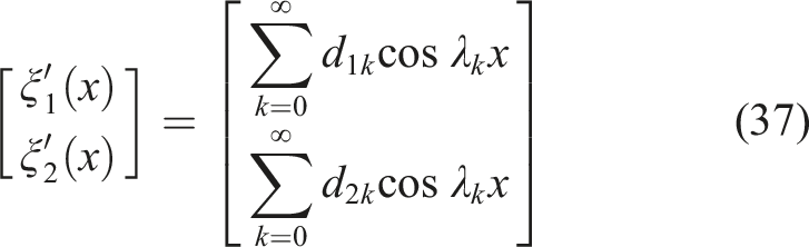
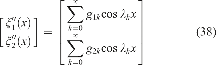
This section will present the solution procedure for the thermoacoustic governing equations and their arbitrary impedance boundaries. The sound pressure and its first-order and second-order derivatives are each expanded into a modified Fourier series form, namely,

$p_1={\displaystyle \sum }_{k=0}^{\infty }{a}_k\cos {\lambda }_{k}x+b_1{\xi }_1\left(x\right)+b_2{\xi }_2\left(x\right)$

(33)

$\frac{d{p}_1}{dx}={\displaystyle \sum }_{k=0}^{\infty }\left(-{\lambda }_k{a}_k\right)\sin {\lambda }_{k}x+b_1{\xi }_1^{\prime }\left(x\right)+b_2{\xi }_2^{\prime }\left(x\right)$

(34)

$\frac{d^2{p}_1}{d{x}^2}={\displaystyle \sum }_{k=0}^{\infty }\left(-{\lambda }_k^2{a}_k\right)\cos {\lambda }_{k}x+b_1{\xi }_1^{″}\left(x\right)+b_2{\xi }_2^{″}\left(x\right)$

(35)

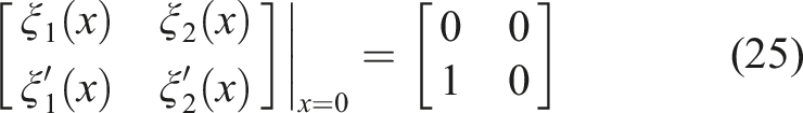
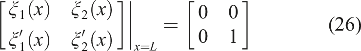
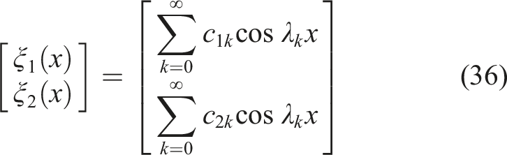
Similarly, the complementary functions and their derivatives are expanded into the Fourier series form as

$\left[\begin{array}{c}{\xi }_1\left(x\right)\\ {\xi }_2\left(x\right)\end{array}\right]=\left[\begin{array}{c}{\displaystyle \sum }_{k=0}^{\infty }{c}_{1k}\cos {\lambda }_{k}x\\ {\displaystyle \sum }_{k=0}^{\infty }{c}_{2k}\cos {\lambda }_{k}x\end{array}\right]$

(36)

$\left[\begin{array}{c}{\xi }_1^{\prime }\left(x\right)\\ {\xi }_2^{\prime }\left(x\right)\end{array}\right]=\left[\begin{array}{c}{\displaystyle \sum }_{k=0}^{\infty }{d}_{1k}\cos {\lambda }_{k}x\\ {\displaystyle \sum }_{k=0}^{\infty }{d}_{2k}\cos {\lambda }_{k}x\end{array}\right]$

(37)

$\left[\begin{array}{c}{\xi }_1^{″}\left(x\right)\\ {\xi }_2^{″}\left(x\right)\end{array}\right]=\left[\begin{array}{c}{\displaystyle \sum }_{k=0}^{\infty }{g}_{1k}\cos {\lambda }_{k}x\\ {\displaystyle \sum }_{k=0}^{\infty }{g}_{2k}\cos {\lambda }_{k}x\end{array}\right]$

(38)

where the process for solving coefficients of the complementary functions and their derivatives is shown in Appendix A.

Substituting equations (33)–(38) into equation (17) will lead to the following equation

$\begin{array}{l}{\displaystyle \sum }_{k=0}^{\infty }\left[-{\lambda }_k^2{a}_k+b_1{g}_{1k}+b_2{g}_{2k}\right]\cos {\lambda }_{k}x-\tau \left\{{\displaystyle \sum }_{k=0}^{\infty }-{\lambda }_k{a}_k\sin {\lambda }_{k}x+{\displaystyle \sum }_{k=0}^{\infty }\left[b_1{d}_{1k}+b_2{d}_{2k}\right]\cos {\lambda }_{k}x\right\}\\ -{\omega }^2\alpha \beta \left\{{\displaystyle \sum }_{k=0}^{\infty }\left[a_k+b_1{c}_{1k}+b_2{c}_{2k}\right]\cos {\lambda }_{k}x\right\}=0\end{array}$

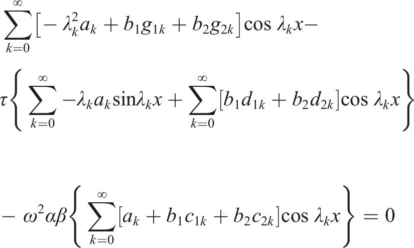
By following the Galerkin method which truncates the modes in the modal space instead of discretizing them over the spatial domain, and using cosλ_nx (n = 0∼k) as the weighting function, the following thermo-acoustic coupling equations can be obtained in matrix form, namely,

${\mathbf{T}}_{\mathbf{1}}\left({\mathbf{F}}_{\mathbf{2}}\mathbf{A}+\mathbf{G}\mathbf{B}\right)-\tau \left({\mathbf{T}}_{\mathbf{2}}{\mathbf{F}}_{\mathbf{1}}\mathbf{A}+{\mathbf{T}}_{\mathbf{3}}\mathbf{D}\mathbf{B}\right)-{\omega }^2\mathbf{\psi }{\mathbf{T}}_{\mathbf{4}}\left(\mathbf{A}+\mathbf{C}\mathbf{B}\right)=\mathbf{0}$

(40)

where

${\mathbf{T}}_1^{k,n}={\int }_0^L\cos \left({\lambda }_{k}x\right)\cos \left({\lambda }_{n}x\right)dx$

(41)

${\mathbf{T}}_2^{k,n}={\int }_{x_l}^{x_r}\sin \left({\lambda }_{k}x\right)\cos \left({\lambda }_{n}x\right)dx$

(42)

${\mathbf{T}}_3^{k,n}={\int }_{x_l}^{x_r}\cos \left({\lambda }_{k}x\right)\cos \left({\lambda }_{n}x\right)dx$

(43)

${\mathbf{T}}_4=\left[\begin{array}{c}{\mathbf{T}}_{4A}\\ {\mathbf{T}}_{4B}\\ {\mathbf{T}}_{4C}\end{array}\right]$

(44)

${\mathbf{T}}_{4A}^{k,n}={\int }_0^{x_l}\cos \left({\lambda }_{k}x\right)\cos \left({\lambda }_{n}x\right)dx$

(45)

${\mathbf{T}}_{4B}={\mathbf{T}}_2$

(46)

${\mathbf{T}}_{4C}^{k,n}={\int }_{x_r}^L\cos \left({\lambda }_{k}x\right)\cos \left({\lambda }_{n}x\right)dx$

(47)

${\mathbf{F}}_1=\left[\begin{array}{cccc}-{\lambda }_0& & & \\ & -{\lambda }_1& & \\ & & ...& \\ & & & -{\lambda }_k\end{array}\right]$

(48)

${\mathbf{F}}_2=\left[\begin{array}{cccc}-{\lambda }_0^2& & & \\ & -{\lambda }_1^2& & \\ & & ...& \\ & & & -{\lambda }_k^2\end{array}\right]$

(49)

$\mathbf{C}={\left[\begin{array}{cccc}{c}_{10}& c_{11}& ...& c_{1k}\\ c_{20}& c_{21}& ...& c_{2k}\end{array}\right]}^{\mathrm{{\rm T}}}$

(50)

$\mathbf{D}={\left[\begin{array}{cccc}{d}_{10}& d_{11}& ...& d_{1k}\\ d_{20}& d_{21}& ...& d_{2k}\end{array}\right]}^{\mathrm{{\rm T}}}$

(51)

$\mathbf{G}={\left[\begin{array}{cccc}{g}_{10}& g_{11}& ...& g_{1k}\\ g_{20}& g_{21}& ...& g_{2k}\end{array}\right]}^{\mathrm{{\rm T}}}$

(52)

$\mathbf{\psi }=\left[\begin{array}{ccc}{\psi }_A& {\psi }_B& {\psi }_C\end{array}\right]$

(53)

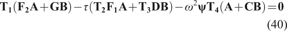
Among them, the calculation method of each coefficient is shown in Appendix A. Substituting equations (29)–(40), the matrix form of the thermoacoustic equation with arbitrary boundary conditions is obtained, namely,

$\left(\mathbf{K}+\omega \mathbf{X}+{\omega }^2\mathbf{M}+{\omega }^3\mathbf{Y}\right)\mathbf{A}=\mathbf{0}$

(54)

where

$\mathbf{K}={\mathbf{T}}_1{\mathbf{F}}_2-\tau {\mathbf{T}}_2{\mathbf{F}}_1$

(55)

$\mathbf{X}=\left({\mathbf{T}}_1\mathbf{G}-\tau {\mathbf{T}}_3\mathbf{D}\right)\mathbf{Z}$

(56)

$\mathbf{M}=-\mathbf{\psi }{\mathbf{T}}_4$

(57)

$\mathbf{Y}=-\mathbf{\psi }{\mathbf{T}}_4\mathbf{C}\mathbf{Z}$

(58)

It can be seen that equation (54) cannot be solved by the conventional method of solving matrix eigenvalues, so it is transformed into the state space matrix equation

$\left(\mathbf{R}-\omega \mathbf{S}\right)\mathbf{H}=\mathbf{0}$

(59)

where,

$\mathbf{R}=\left[\begin{array}{ccc}\mathbf{0}& \mathbf{E}& \mathbf{0}\\ \mathbf{0}& \mathbf{0}& \mathbf{E}\\ \mathbf{K}& \mathbf{X}& \mathbf{M}\end{array}\right]$

(60)

$\mathbf{S}=\left[\begin{array}{ccc}\mathbf{E}& \mathbf{0}& \mathbf{0}\\ \mathbf{0}& \mathbf{E}& \mathbf{0}\\ \mathbf{0}& \mathbf{0}& -\mathbf{Y}\end{array}\right]$

(61)

$\mathbf{H}=\left[\begin{array}{c}\mathbf{A}\\ \omega \mathbf{A}\\ {\omega }^2\mathbf{A}\end{array}\right]$

(62)

here, E is the unit matrix.

By solving the eigenvalues of equation (62), the critical frequency can be found, and the coefficient matrix A corresponding to the frequency is the amplitude coefficient corresponding to the sound pressure so that the sound pressure distribution can be found in its entirety,

$p_1\left(x\right)={\mathbf{N}}_1\left(\mathbf{E}+\omega \mathbf{C}\mathbf{Z}\right)\mathbf{A}$

(63)

where

${\mathbf{N}}_1=\left[\begin{array}{cccc}\cos {\lambda }_{0}x& \cos {\lambda }_{1}x& ...& \cos {\lambda }_{k}x\end{array}\right]$

(64)

Similarly, from the above derivation and equation (12), the volume flow rate distribution can be written as

$U_1\left(x\right)=\frac{-1}{\omega \alpha }\left({\mathbf{N}}_2{\mathbf{F}}_1+\omega {\mathbf{N}}_1\mathbf{D}\mathbf{Z}\right)\mathbf{A}$

(65)

where

${\mathbf{N}}_2=\left[\begin{array}{cccc}\sin {\lambda }_{0}x& \sin {\lambda }_{1}x& ...& \sin {\lambda }_{k}x\end{array}\right]$

(66)

Equations (63) and (66) allow the distribution of the modal acoustic pressure and volume flow rate along the x-axis corresponding to the oscillation frequency to be derived, and these two parameters can be more useful for analyzing the dynamics of the thermoacoustic engine. In addition, other parameters based on the distribution of sound pressure and volume flow rate, such as heat flow, can also be solved arithmetically and will not be discussed here. In this paper, the oscillating frequency, sound pressure, and volume flow rate modal distributions are used as the physical characteristics of the thermoacoustic engine to study the influence of each parameter on it.

Results and discussions

This section will first check the stability of the method proposed in this study and then verify the accuracy of the method by comparing the results with those obtained from other approaches in literature. On this basis, the trends of oscillation frequencies of the four working gases and the modal distributions of sound pressure and volume flow rate of H₂ with engine length, stack length, stack position, and arbitrary boundary conditions are investigated and discussed.

Model validation

The modified Fourier series adopted in this work needs to be truncated during the practical simulation, and the term of the truncation number affects the accuracy of the solution. Therefore, the impact of truncation on the results needs to be judged before the results are verified. In the present work, a parametric study of a one-dimensional thermoacoustic engine with the following parametric characteristics is carried out. The structure and environmental parameters of the thermoacoustic engine studied in this paper are shown in Table 1. The physical parameters of the four working fluids studied in this paper were used by Boroujerdi and Ziabasharhagh (2016). This set of parameters is still adopted in the subsequent simulation discussions.

Table 1.

Structure and environmental parameters of the studied thermoacoustic engine.

L (m)	D (m)	xl (m)	xr (m)	l (mm)	y0 (mm)	Th (K)	Tc(K)	pm(MPa)
1	0.05	0.05	0.1	5	5	600	300	1

To investigate the effect of the truncation number on the accuracy of solving the critical frequency of the thermoacoustic engine, here truncation numbers are taken as k = 5, k = 10, k = 15, k = 20, and k = 25, and the obtained modal frequency results are shown in Table 2.

Table 2.

The first 10 modal frequencies with different series truncation numbers k (Hz).

Modal order	$k=5$	$k=10$	$k=15$	$k=20$	$k=25$
1	682.89	682.85	682.85	682.85	682.85
2	1364.66	1364.26	1364.26	1364.26	1364.26
3	2044.47	2042.69	2042.67	2042.67	2042.67
4	2723.36	2716.88	2716.81	2716.81	2716.81
5	3415.97	3386.30	3386.04	3386.04	3386.04
6	─	4051.75	4050.83	4050.83	4050.83
7	─	4715.92	4713.10	4713.07	4713.07
8	─	5383.57	5375.70	5375.57	5375.57
9	─	6063.37	6041.28	6040.88	6040.88
10	─	6816.77	6711.30	6710.27	6710.27

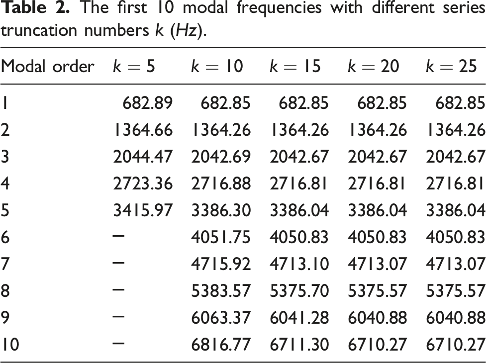
From the results presented in Table 2, it can be seen that with the increasing number of truncations, the modal frequency sought has a trend of constant change until stability. The modal frequency of the first 10 orders stabilizes at the truncation number k = 20 and remains constant at k = 25. The thermoacoustic engine often operates at the first-order intrinsic frequency, also called onset frequency, therefore, in the subsequent parameter study, the truncation number k = 25 is used as a precondition to ensure the accuracy of the critical frequency and dynamic parameters.

Using the model established in this work, the critical oscillation frequencies of the system at the oscillation temperature are calculated to verify the unified solution of the dynamical behavior of 1D thermoacoustic engine based on the modified Fourier series method, and the pure acoustic frequencies for the same structural parameters are also listed in Table 3.

Table 3.

Comparison of the first four orders of critical frequencies of thermoacoustic engines with the results of reference and pure acoustic frequencies (Hz).

		1st mode	2nd mode	3rd mode	4th mode
Acoustic model		658.0	1316.1	1974.1	2632.2
TA model	Reference	674.8	1346.4	2017.9	2700.5
	Present	679.4	1357.3	2032.3	2703.0
	Difference	0.68%	0.81%	0.71%	0.09%

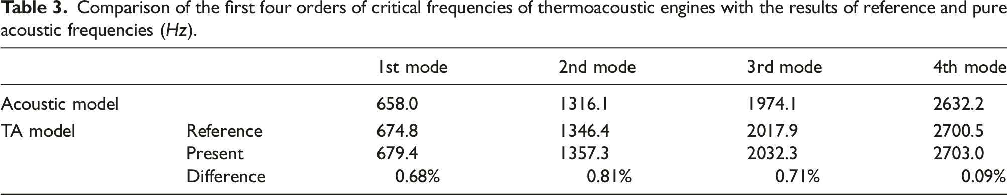
The critical frequencies available in literature are derived under the model condition that the two ends of the thermoacoustic heat engine are closed. In this paper, the boundary impedance values at both ends are set to Z to simulate the two-end closure condition. From Table 3, it can be seen that the difference between the results of this paper and the results of the reference literature are within 1% at the same temperature. It can also be seen that the modal frequencies in the thermoacoustic model differ significantly from the pure acoustic frequencies, which is caused by the existence of the stack, the introduction of the heat source excitation term, and the corresponding heat transfer and viscous losses.

To show the difference between the thermoacoustic model and the pure acoustic model more visually, the sound pressure distribution at the first four orders of modal frequencies of both is plotted in Figure 2.

Figure 2.

Comparison of sound pressure modal distribution between pure acoustic model and thermoacoustic model.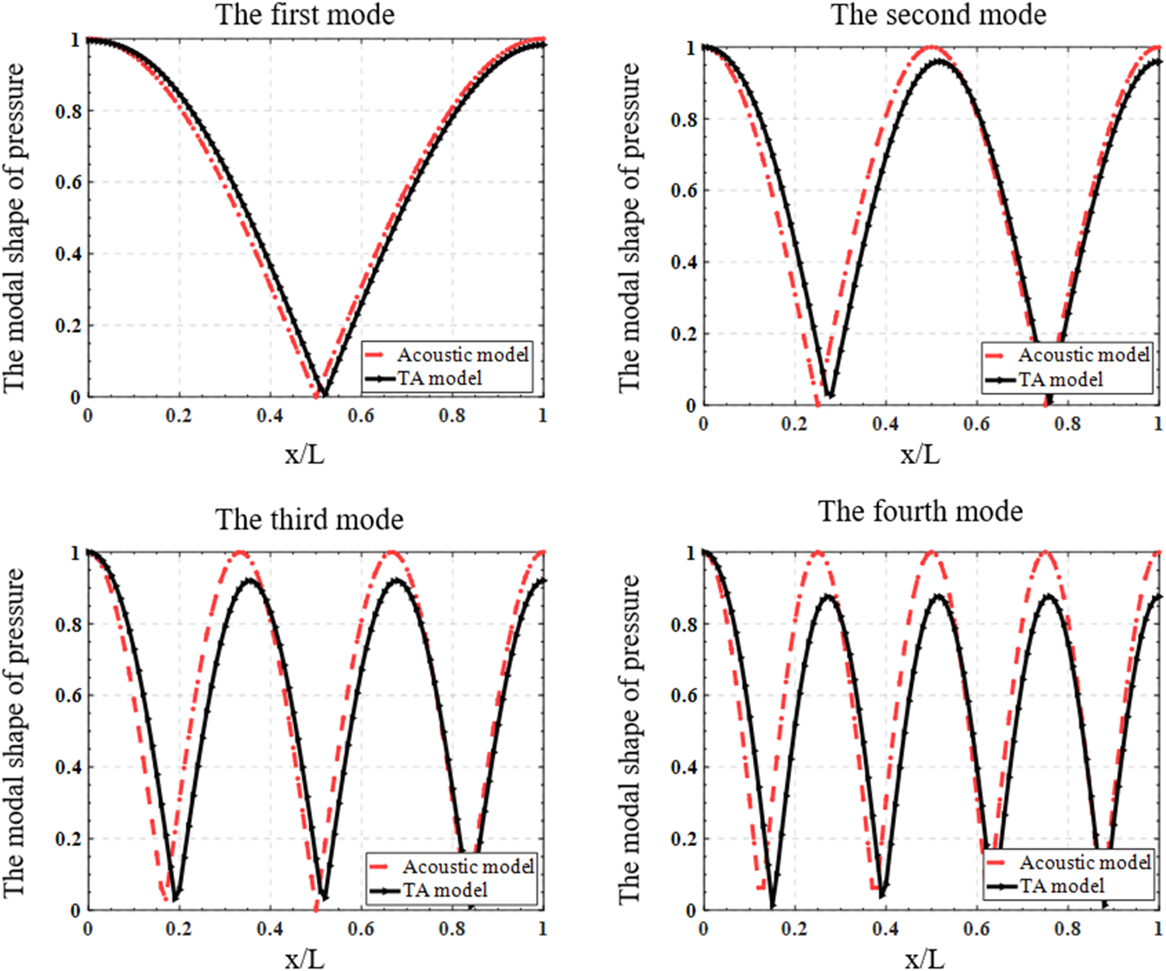

Figure 2 visualizes the change in the modal distribution of the acoustic pressure after introducing the heat source excitation term in the tube and considering the heat transfer and viscous losses. For the first-order modal distribution, the difference is not very significant, but only causes a slight rightward shift of the acoustic pressure node. For the other modal distributions after the first order, not only the rightward shift of the nodes is caused but also the decay of the modal amplitude of the sound pressure, which is due to the partial energy dissipation caused by the consideration of heat transfer and viscous losses, thus causing the decay of the modal amplitude of the sound pressure.

Influence of engine length

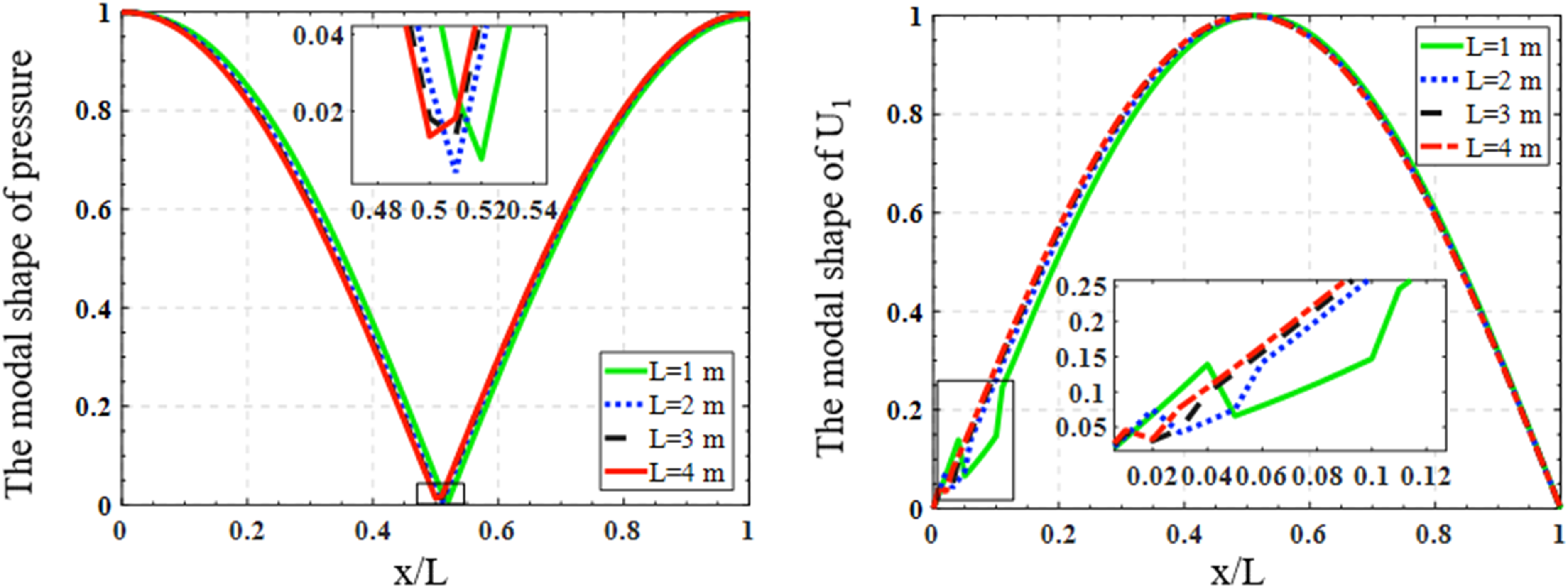
The effect of engine length on the first-order modal frequency of the four working gases while keeping the position of the stack constant is shown in Figure 3, and the effect on the modal distribution of acoustic pressure and volume flow rate of H₂ gas is shown in Figure 4.

Figure 3.

Effect of engine length on the onset frequency of the four working fluids.

Figure 4.

Effect of engine length on sound pressure and volume flow rate distribution.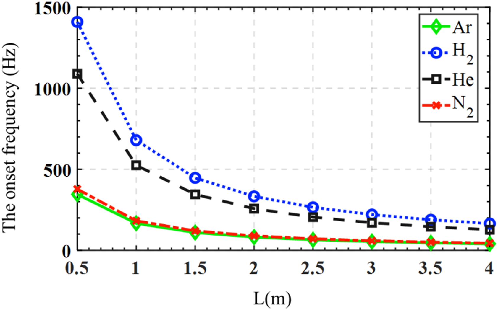

From Figure 3, the effect of the variation of engine length on the onset frequency of the four working fluids is obvious, that is, the onset frequency is inversely proportional to the engine length. Among the four working gases, H₂ has a higher onset frequency, and the onset frequency is more affected by the engine length variation. N₂ and Ar have similar onset frequencies. Therefore, in the design work of thermoacoustic engines, the operating frequency and the engine construction cost need to be considered together. While longer engine lengths result in lower operating frequencies, they also cost more to build. In particular, for the thermoacoustic engine with H₂ as the working gas, the effect of the engine length on the sound pressure and volume flow rate distribution is represented in Figure 4.

From the diagram of sound pressure distribution, it can be concluded that the length of the engine has less of an effect on the sound pressure modal distribution. Its microscopic diagram also reveals that the sound pressure nodes are slightly shifted around the half-engine length, which is intended to make the offset of the acoustic pressure nodes more obvious. In the volume flow rate distribution diagram, the engine length has a more obvious effect on its modal distribution. The relative length of the stack shortens as a result of the relative engine lengthening under the condition that the stack position remains constant, which has a lessened impact on the internal flow field’s volume flow rate. Equation (11) in the modeling process represents the viscous loss of the stack to the fluid field. From the perspective of physics, as the relative length of the stack decreases, its viscous loss to the fluid field diminishes, and as a consequence, the relative magnitude of volumetric flow rate decay decreases. This can be confirmed by the microscopic diagram of volume flow rate distribution in Figure 4.

Influence of stack length and position

In this work, the length of the stack is changed by keeping the position of the left side of the stack the same and changing the position of the right end. The variation of the onset frequency with the length of the stack for the four working gases is plotted in Figure 5, and likewise, the modal distribution of the sound pressure and volume flow rate in the engine with H₂ as the working gas as a function of the stack length is given in Figure 6.

Figure 5.

Effect of the stack length on the onset frequency of the four working fluids.

Figure 6.

Effect of the stack length on sound pressure and volume flow rate distribution.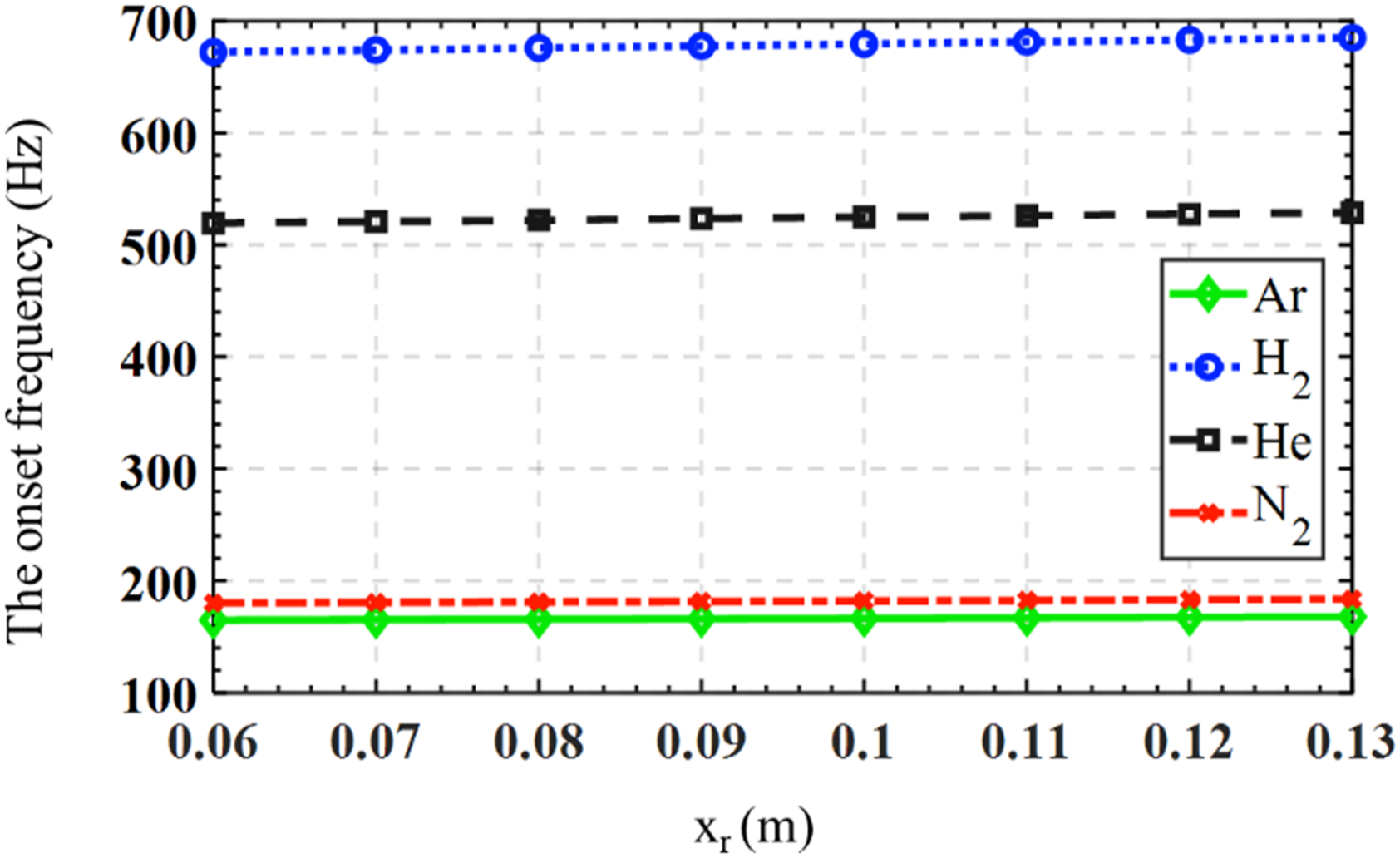

In contrast to the effect of engine length on the onset frequency of the four working fluids, it can be observed that while the stack length has less effect on the onset frequency, as the length of the stack increases, the onset frequency exhibits an increasing trend; though, the increase is not statistically significant. This is due to the fact that when temperatures of the high-temperature heat source and the low-temperature ambiance are fixed, with an increase in the length of the plate stack, the temperature gradient along the plate stack will decrease, which makes it easier for the thermoacoustic engine to enter a state in which it is unable to generate vibrations; alternatively, when after the vibrations have been generated, the performance of the engine is severely diminished. This situation makes it impossible to vary the range of plate stack length excessively, and within the range of variation specified in this paper, the onset frequency is only slightly altered.

The length of the stack has little effect on the modal distribution of acoustic pressure depicted in Figure 6, whose nodes are all on the right side of the half-engine length as a result of introducing the stack. Due to the fixed position of the left side of the stack, the distribution to the left of the stack overlaps. As a corollary, the distribution mode of the volume flow rate can be observed to be more dissimilar than others. The volume flow rate of the fluid within the stack varies to a different extent, but the progressing trend remains the same. This is to the variations in the length of the plate stack. Outside the stack, the distribution mode becomes similar to others again.

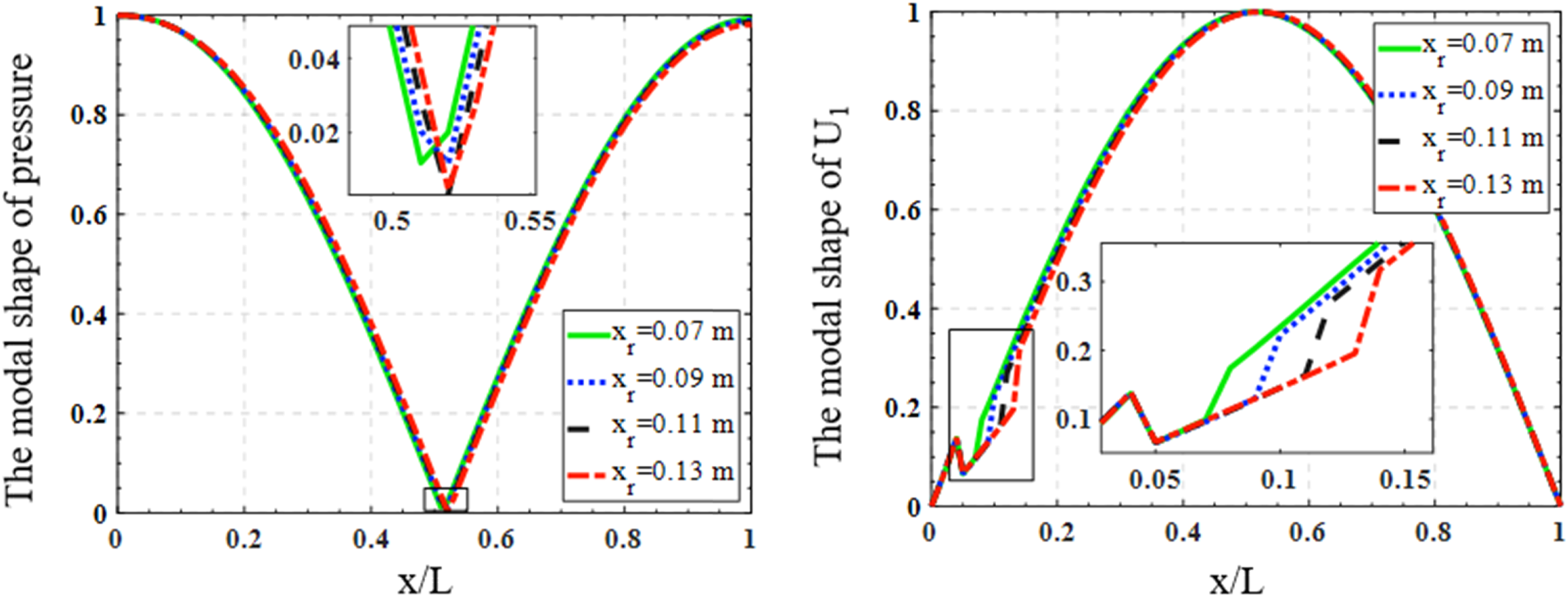
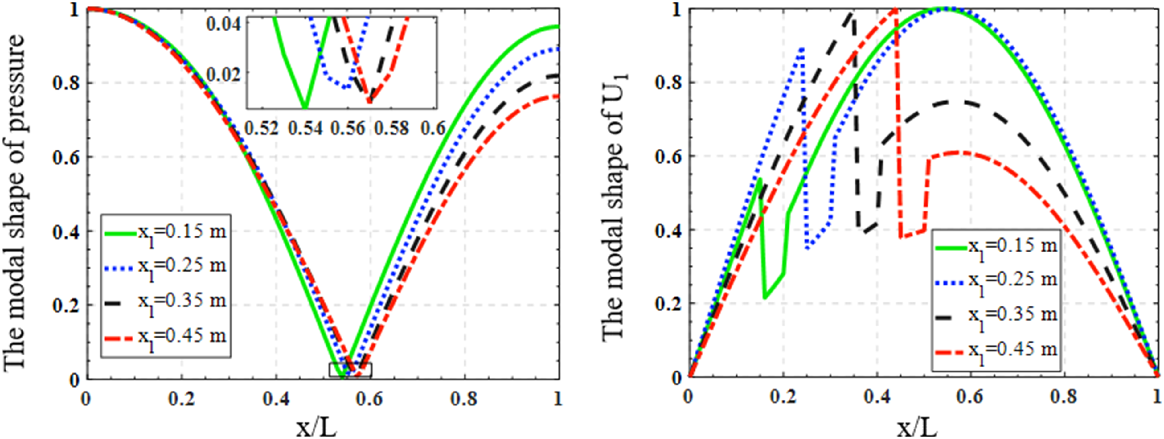
Under the assumption that the length of the plate stack and other factors remain constant, the position change on the left side of the plate stack is regarded in this paper as the position change of the plate stack. Figures 7 and 8 depict, respectively, the variation of the oscillation frequencies of the four fluids, the modal distributions of the acoustic pressure, and the volume flow rate of the hydrogen working gas with stack position.

Figure 7.

Effect of the stack position on the onset frequency of the four working fluids.

Figure 8.

Effect of the stack position on sound pressure and volume flow rate distribution.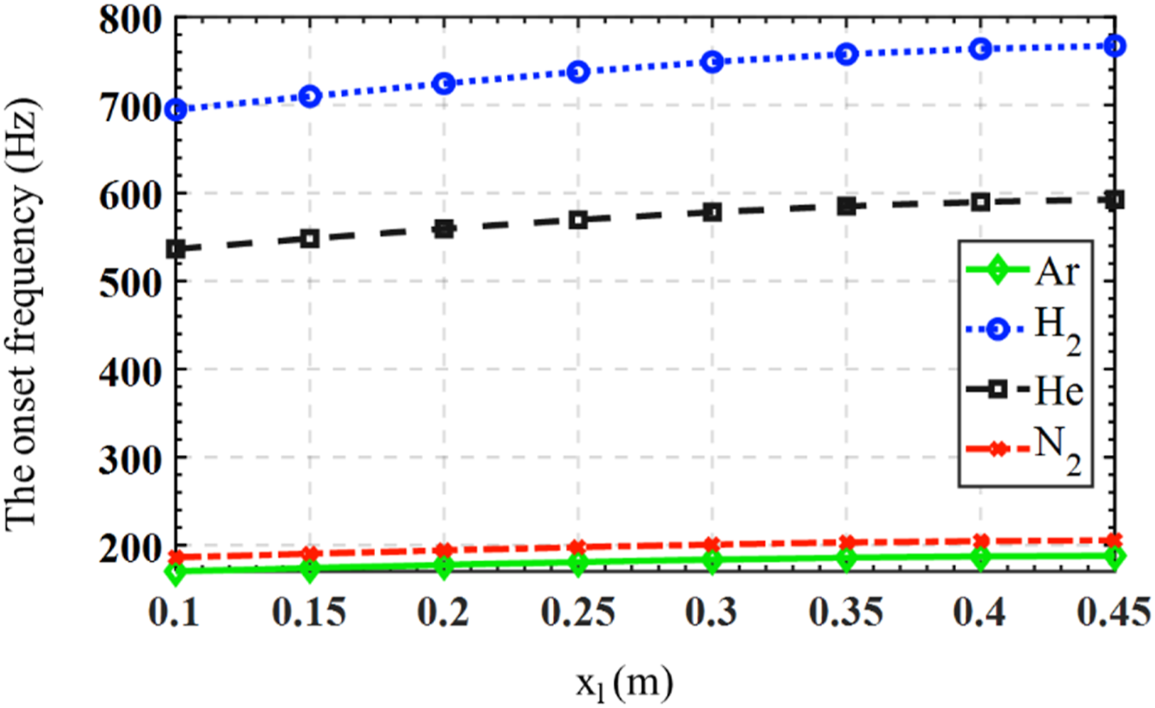

The trend of the curve in Figure 7 indicates that the onset frequency of each fluid increases proportionally to the distance of the stack from the buffer end of the thermoacoustic engine. In addition, the left end of the stack shifts from 0.1 m to 0.45 m, and the oscillation frequency of H₂ increases by nearly 70 Hz. It is essential to explain why the stack position is utilized as the variation range in the figure. The thermoacoustic engine has a prerequisite for the stack position, designed to meet the slightly shorter length of the buffer section to ensure that as little useful high-temperature heat source energy is lost as possible in the buffer section. This results in an impossibly large range of variation in stack length.

The acoustic pressure mode distribution curves in Figure 8 vary significantly with the position of the stack, and the node positions vary significantly. The rightmost acoustic pressure mode amplitude decreases proportionally to the distance of the stack from the buffer end. This is because there is less space on the right side of the stack for the acoustic pressure mode amplitude to develop. The modal distribution of the volume flow rate varies significantly more with plate stack position. The closer the stack is to the resonator end, the greater the difference in the modal distribution of the volume flow rate between the two sides of the stack, and the smoother the development of the stack.

Influence of boundary conditions

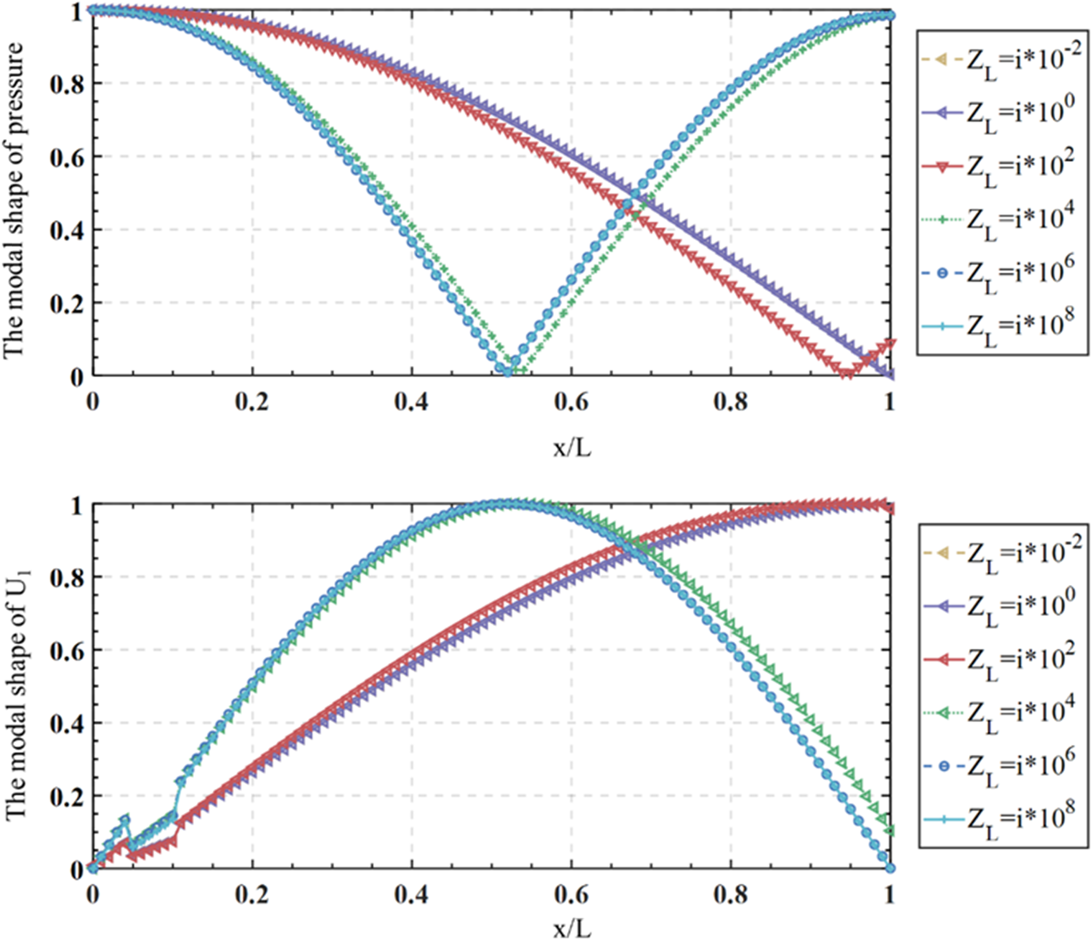
One of the advantages of the proposed unified solution method based on improved Fourier series is that it can model arbitrary boundary conditions with boundary impedances Z. Since actual thermoacoustic engines often have a structure with one end closed and the other end closed or connected to a transducer, the effect of boundary conditions on their dynamical behavior is investigated in this section for the left end of the engine as the closed end and the right end as either impedance boundary. The effects of arbitrary boundary conditions on the four working fluid onset frequencies and on the modal distribution of the H₂ acoustic field are illustrated in Figures 9 and 10, respectively.

Figure 9.

Effect of the boundary conditions on the onset frequency of the four working fluids.

Figure 10.

Effect of the boundary conditions on sound pressure and volume flow rate distribution.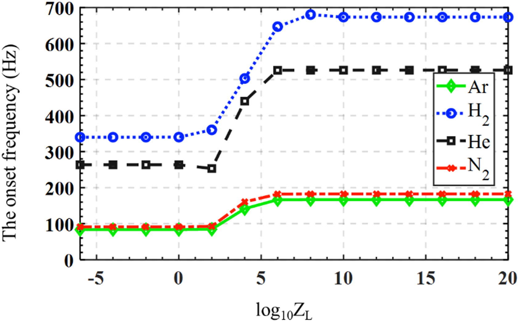

According to Figure 9, the trend of the four working fluids with the boundary conditions can be divided into three regions: the first region is Z_L = 10⁻⁶–10⁰, in this region, the engine boundary condition is open and its onset frequency is maintained at a stable level. The second region is Z_L = 10⁰–10⁸, where appears a considerable fluctuation of the onset frequency, and in the third region, i.e., Z_L = 10⁸–10²⁰, the onset frequency remains constant again. The fact that the onset frequency in the third region is consistent with the results of the verification session demonstrates that the third region corresponds to the case where both sides of the engine are closed. In this model, Z_L = 10⁰ corresponds to the simulated open case, while Z_L = 10⁸ corresponds to the simulated closed case; additionally, when the impedance value falls between these two values, it is regarded as the simulated elastic wall for simulating boundary conditions such as connecting an external transducer.

Six boundary cases are extracted in Figure 10 in order to investigate their effects on the modal distribution of acoustic pressure mode and volume flow rate. It can be determined from the acoustic pressure mode distribution that when Z_L = 10⁻², the boundary case is an open boundary, and the difference between it and the modal distribution at Z_L = 10² can be observed. When Z_L = 10⁶, the stage boundary is in region 2, but it is close to the closed condition; therefore, its difference from the modal distribution of Z = 10⁸ is smaller. From the volume flow rate modal distribution diagram, the difference between the open and closed boundary becomes more apparent. Notably, under the open boundary condition, the distribution of volume flow rate at the stack varies more smoothly.

Conclusion

In this paper, a unified solution of thermoacoustic engine modal frequency and its dynamic behavior under arbitrary boundary conditions is proposed. Based on the assumption of linear acoustics and heat transfer and viscous dissipation functions, the classical thermoacoustic control equations are reconstructed by using a modified Fourier series to establish the functional relationships between the modal frequency, acoustic pressure mode, and other parameters of the thermoacoustic system, and after using Galerkin method, the analytical solution of the oscillation frequency is obtained by solving the characteristic equation of the oscillation frequency for a given temperature difference, and then the modal distributions of acoustic pressure and volume flow rate are obtained. On this basis, the effects of some structural parameters and boundary conditions on the modal frequencies and the modal distributions of sound pressure and volume flow rate of different working gases are investigated, and the specific conclusions are as follows:

(1). On the basis of the original linear thermoacoustic assumptions, a modified Fourier series is used to solve the derivative discontinuity of sound pressure at the boundary conditions. Then, the governing equations in thermoacoustics under arbitrary impedance boundary conditions are transformed into the eigenvalue equations for the oscillation frequency, the sound pressure series coefficients and other parameters using the Galerkin method. This transformation can directly infer the oscillation frequency and the distribution modes of sound pressure and volume flow rate. The advantages of the proposed method include low consumption of computational resources and applicability under arbitrary boundary conditions. This study can serve as a good reference for the pre-design work of TAEs.

(2). There exists a significant inverse relationship between the length of the engine and the modal frequencies of the various operating gases. The displacement of the node position of the acoustic pressure modal distribution is caused by the difference in engine length. The modal distribution of volume flow rate at the stack varies significantly as engine length changes, but engine length has no effect on its development trend within the plate stack. There is a trade-off between the type of working gas, the cost of the engine, and the frequency of operation when designing a thermoacoustic engine.

(3). The length of the stack influences the onset frequency of various working gases; the longer the length, the higher the onset frequency; however, the growth amplitude is insignificant. The variation in stack length also results in the offset of the nodes of the acoustic pressure mode distribution, while the trend of the volume flow rate distribution within the stack is unaffected.

(4). The position of the stack has a significant effect on the modal frequency of various working gases; for instance, in the case of H₂, the offset of 0.35m position causes the onset frequency to increase by nearly 70Hz. The effect of stack position on the mode distribution of acoustic pressure and volume flow rate is highly significant. The greater the offset of the acoustic pressure mode node, the closer the position of the stack is to the resonator end; while the amplitude of the acoustic pressure mode on the right side of the engine decreases, and the development trend of the volume flow rate mode within the stack becomes smoother.

(5). The boundary impedance can be used to describe the boundary conditions; in this model, the value of 10⁰ is used to describe the open boundary and the value of 10⁸ is used to describe the closed boundary. The boundary impedance value can be arbitrarily varied to simulate from the open boundary to the rigid wall and all intermediate cases, laying the groundwork for future research on the coupling of thermoacoustic engines with other loads or transducers.