
Abstract
Aiming at operating optimally minimizing error of tracking and designing control effort, this study presents a novel generalizable methodology of an optimal torque control for a 6-degree-of-freedom Stewart platform with rotary actuators. In the proposed approach, a linear quadratic integral regulator with the least sensitivity to controller parameter choices is designed, associated with an online artificial neural network gain tuning. The nonlinear system is implemented in ADAMS, and the controller is formulated in MATLAB to minimize the real-time tracking error robustly. To validate the controller performance, MATLAB and ADAMS are linked together and the performance of the controller on the simulated system is validated as real time. Practically, the Stewart robot is fabricated and the proposed controller is implemented. The method is assessed by simulation experiments, exhibiting the viability of the developed methodology and highlighting an improvement of 45% averagely, from the optimum and zero-error convergence points of view. Consequently, the experiment results allow demonstrating the robustness of the controller method, in the presence of the motor torque saturation, the uncertainties, and unknown disturbances such as intrinsic properties of the real test bed.
1. Introduction
In applications where higher acceleration and velocity and better accuracy and lighter weight are essential or where a comparatively high bearing capacity per robot weight is required, parallel mechanisms are alternatively preferred to serial manipulators (Taghirad 2013, Tajdari et al. 2017b). Namely, some of the applications are space interferometry, spacecraft communication devices (Furqan et al., 2017), flight simulator (Huang et al., 2016), surgery (Orekhov et al., 2016) production line, and scanning (Huang et al., 2018). Among the other things, the high accuracy scanning of the human body for the purpose of surgeries, designing anatomical adaptable rehabilitation devices (Nomura et al., 2016), and next generation of Ultra Personalized Products and Services (UPPS) (Kwon and Kim 2012, Yang et al. 2020) attract more attention. It shows the importance of health and humanity survival and how it is influenced by robots’ high precision. One of the interesting scanning scenarios is fast automated breast scanning (Chen et al. 2015, Merouche et al. 2015, Sun et al. 2018) which is supposed as the future application of this study. However, because of the flexibility and deformation of the breast tissue, it is a very complex action. The needs of such robots are revealed especially during motion scanning.
High accuracy needs good knowledge of kinematic, dynamic, and control of a parallel robot to investigate complex dynamic and accordingly sophisticated control approaches (Shoham et al., 2003). Well-known parallel robots with wide usage in the aforementioned applications were extracted from the mechanism presented by Gough (1962) and Stewart (1965) based on the fundamental of the recent parallel robots.
Addressing the first issue, solving the kinematics of the parallel robots is considerably complicated because they do not have a definite solution. Also, there is no closed form for these kinds of equations (Sosa-Méndez et al., 2017). Kinematics of the robot with linear manipulator was widely studied in recent years, namely Geng et al. (1992); Petrescu et al. (2018); and Tajdari et al. (2020c), whereas mechanisms with rotary actuators are less studied due to additional complexity of rotation. Thus, in this article, a Stewart robot with rotary manipulator is investigated, owing to the fact that it is faster than a Stewart platform with linear actuators in control responses (Van Nguyen and Ha, 2018). Also, it has less production and maintenance cost, less weight, easier installation procedure (e.g., surgical goals), and powerful ability of integration with other mechanisms (Patel et al., 2018).
Regarding the complex mechanism, the kinematic equation of the robot is a key to dynamical analysis of the parallel robot. In addition, main challenges in the deriving of the dynamic equations are the relationship description between internal or external forces and torques, the states of end effector for controller design, and feasibility study of the robot. Considering the dynamical analysis, several approaches were used such as the comprehensive approach based on momentum (Lopes, 2009), the Newton–Euler methodology (Dasgupta and Mruthyunjaya, 1998), and the Lagrangian approach (Bingul and Karahan, 2012). Furthermore, based on the assumptions for using either of the approaches, different solutions were proposed. One of the solutions assumed dynamic simplifications to the robot such as ignoring friction joints in the links and concluding a basic legs dynamic Do and Yang (1988), Fichter (1986), Merlet (1990), Sugimoto (1989). Some other studies, such as Dasgupta and Mruthyunjaya, 1998), developed a generalized model according to the Newton–Euler formulation to study the effectiveness of the viscous friction in the joints. Also, the Lagrange formulation was used in Lebret et al. (1993).
To assess the automation and the equation of motions, and because there are nonlinearity and uncertainty in the fabricated robot, a computing software capable of simulating inverse kinematic, dynamic motion, and state variable is necessary. To this end, ADAMS is used in this study. The aforementioned software was also used in Cafolla and Marco (2015), Gough (1957), and Stewart (1965). Accordingly, a proper ADAMS model is used in the current article based on the proposed model in Tajdari et al. (2020b). This model is capable to verify any controller approach for the rotary robot dynamic.
The main objective of controller design in parallel robots is to move end effector of the robot precisely, so that it can follow a desired trajectory and orientation of dynamic or static variables (Merlet, 2006). There are many control schemes, which are based on the models and applicable for linear manipulator Stewart robots, namely optimal feedback linearization control (Tajdari et al. 2021a; Tourajizadeh et al. 2016), control of inverse dynamic (Lee et al., 2003), backstepping tracking adaptive control (Huang and Fu, 2004), sliding mode, and PID controllers (Kizir and Bingul 2012; Tajdari et al. 2017a), whereas there are less control approaches for a rotary Stewart robot due to the additional complexity of the robot’s dynamic. Moreover, in the most of the latter methods, controlling the length of links in the robots was used to control the states of the end effector. As a result, a comprehensive methodology for direct controlling from manipulators to the end effector was missed. Consequently, using the position control methodology solely limits the robot design to the joint space (Hopkins and Williams, 2002). In particular, the control methodologies based on the inverse dynamic are substantial to control the end effector motion through the manipulators, directly. Then, there is the possibility of investigating experimental constraints, for example, manipulator saturation, and uncertainty considerations. However, there are limited studies discussing the rotary robot torque control.
Thus, this article aims to develop and test a novel integral torque control methodology for the complicated parallel mechanism to optimize the torques and minimize the tracking error. This is an opening for further implementation of identification approaches, nonlinear control methods, and impedance manipulator control (Yang et al., 2019). The scientific contributions of this article are as follows: Introducing the design architecture of the robust integral controller integrated with an anti-windup scheme, which solves unknown disturbances and manipulator saturation; Integrating an intelligent optimizer gain tuner in the metric for establishing a robust optimal controller with faster zero-error convergence performance; Extensively investigating the sensitivity level, robustness, and attraction region of the controller parameters, and demonstrating the global stability of the controller, which guarantees the global zero-error convergence; and Implementing the controller on a reliable nonlinear system, via ADAMS to validate the robustness, and convergence in different scenarios and also on a fabricated Stewart robot to assess the performance in presence of naturalistic disturbance, manipulators’ saturation, and uncertainties.
An introductory version of this study was presented in Tajdari et al. (2020b), which is collaborated here with a more rigorous concept; a comprehensive demonstration on stability of controller properties for the suggested control law; investigation on level of robustness with respect to parameter choices through numerical experiments; and additional numerical experiments, containing a scenario which presents a state-of-the-art conventional control methodology and a scenario, which includes additional disturbances through the fabricated robot.
2. Stewart platform: Dynamical equations
To derive the equations of motion of a Stewart mechanism, kinematics and kinetics analyses of the dynamical system are required. This step is crucial toward obtaining the relationships between the position and the velocity of the end effector before dynamic analysis.
2.1. Kinematics equation
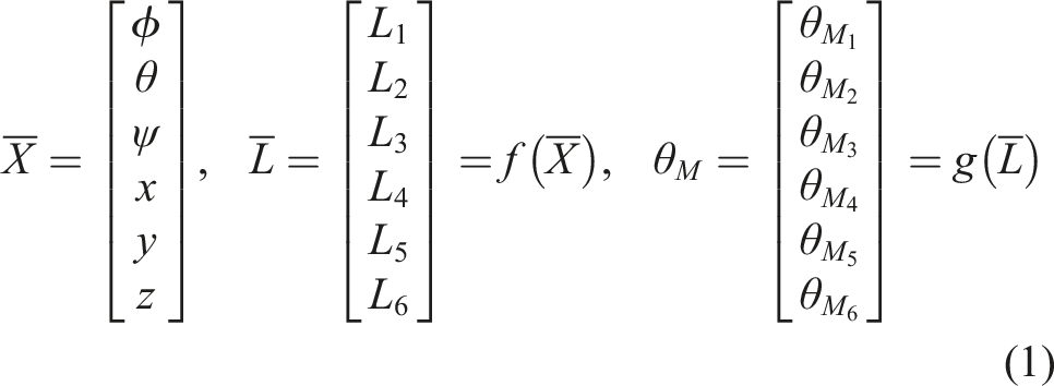
In a Stewart platform which is actuated with rotary motors, controllable variables are the output torques of motors and their rotational angels. In the following equations, a relationship between the motors’ variables and the position of the end effector is presented
Vector Schematic of a Stewart platform. (a) Defined variables and vectors. (b) Dynamic force–torque diagram.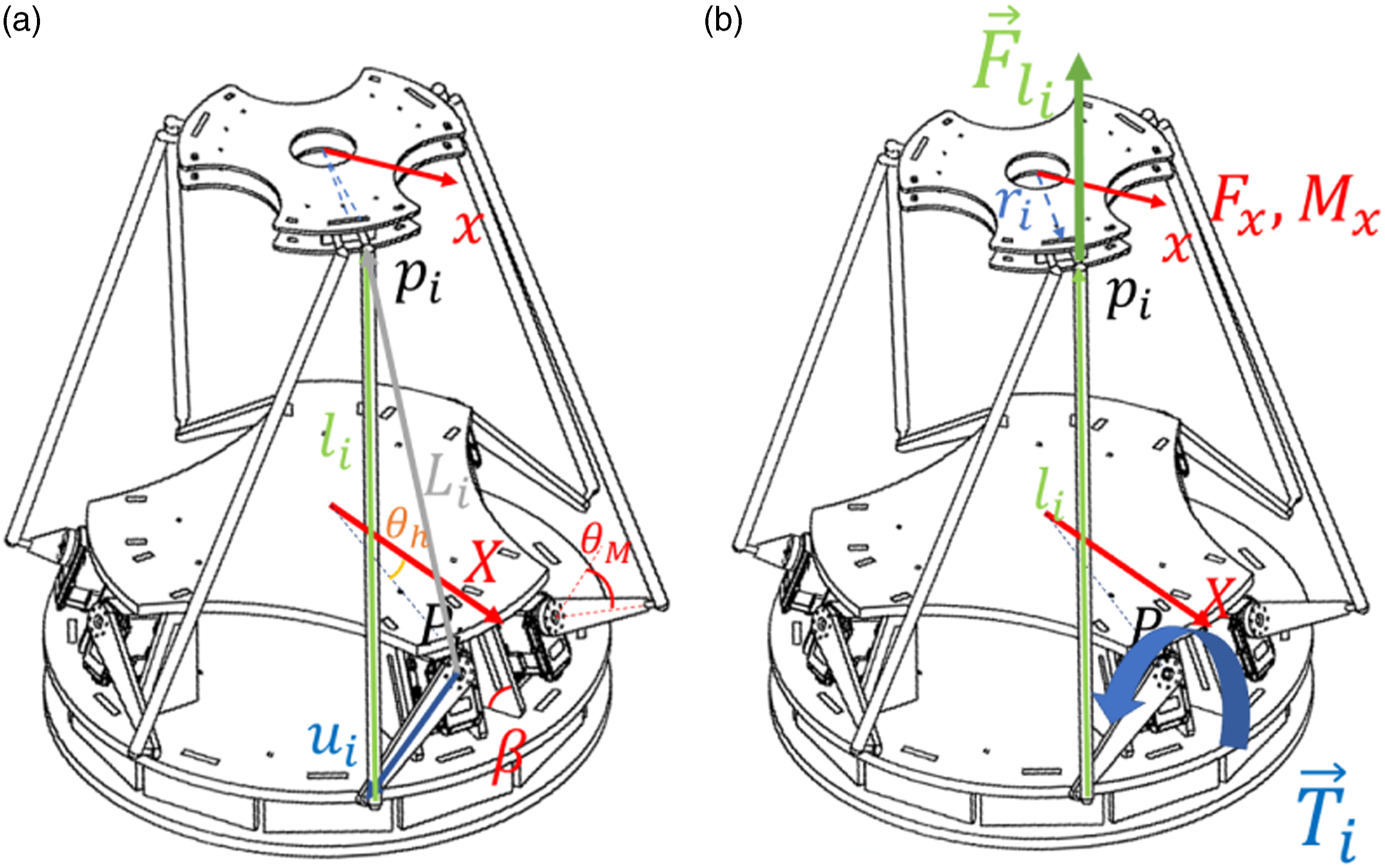


Considering the length of each legs in equation (2), the length of each link connecting the end effector to the base is written as

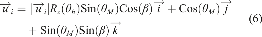
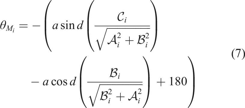

Equation (7) defines that practically having the
2.2. Kinetics equations
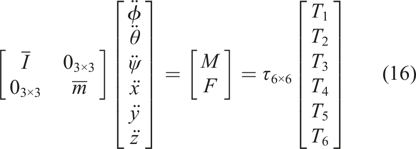
In this section, the dynamical equations of a Stewart platform actuated by six rotary motors are obtained using the Newton–Euler method. The derivations are summarized just to show different dynamic features of the systems and the effects. Figure 1(a) shows a Stewart mechanism with six rotary motors as actuators. As it can be seen, the platform consists of a moving plate as the end effector, a fixed plate as the base, and six legs connected to six rotary actuators, as the manipulators to move the end effector. The spherical joints are used to connect the six legs, the end effector, and the base. The kinetics equations for the end effector can be written as


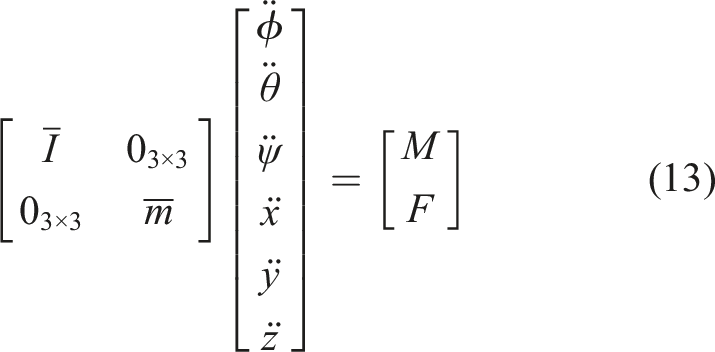

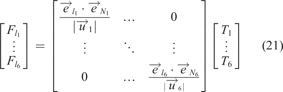
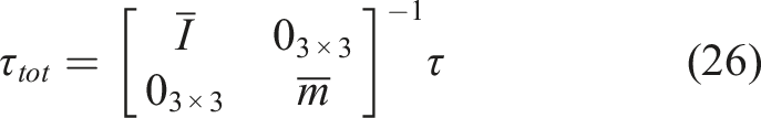
In Figure 1(b), M and F represent the torques and the exerted forces on the end effector, respectively. Addressing the rotary motors’ manipulated torques, the dynamic equation should be derived as a controllable variable–torque relationship discussed in the following

Thus

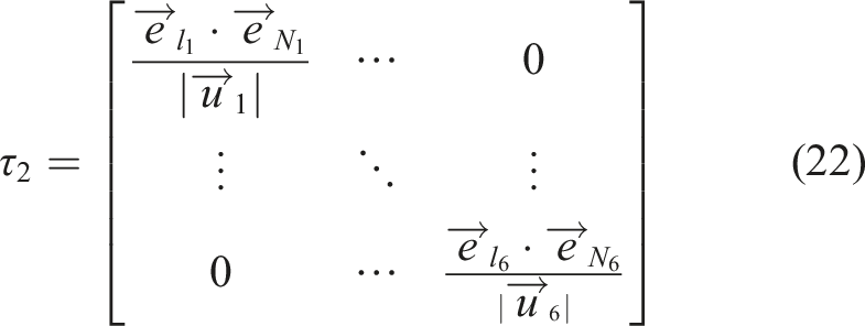
As
Considering
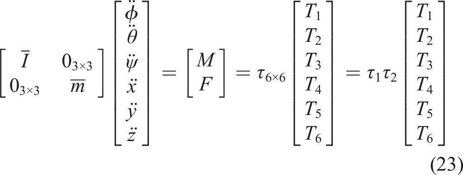
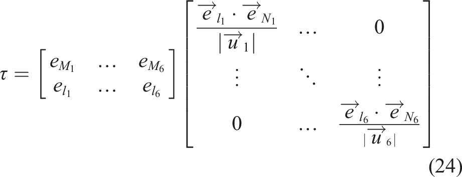
Thus, the ultimate dynamic transfer matrix, from the end effector to the base, can be obtained as

2.3. Evaluation of equations of motion and derivation of the nonlinear model
Providing a valid nonlinear model, which is able to represent the actual system, is crucial for the controller design and evaluation process. Some physical constraints such as collision of objects, hardness and elasticity of rigid bodies, and friction between hard surfaces could not be addressed in MATLAB. Therefore, ADAMS is used to simulate the Stewart model. However, lacking the capability of coding and implementation of different control methods in ADAMS makes it an insufficient tool for evaluating the system. To overcome this problem, MATLAB and ADAMS are connected together to implement the online control method on MATLAB and evaluate the controller performance on the nonlinear system modeled in ADAMS.
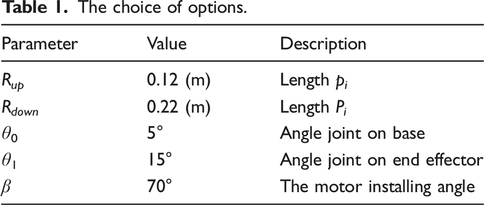
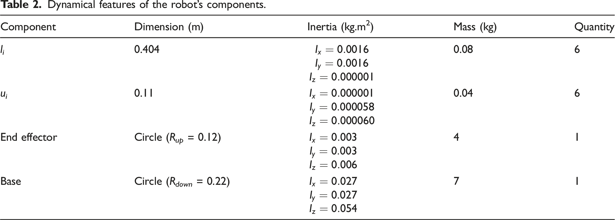
First, the 3D model of the system is designed in SolidWorks (Figures 2 (a) and (b))). Next, the 3D model is imported into the ADAMS and then the essential constraints such as joint types, materials and densities of the bodies, rigidity of them toward each other, and frictions between hard surfaces are applied to the modeled robot. Tables 2 and 1 show the considered values and assumptions for the design variables. As it is reported in Table 2, the system consists of 14 components of mass and moment of inertia. Figure 2(c) shows all the applied constraints to the 3D model. As shown, a bidirectional torque, represented by red vectors, is applied on each leg. 3D model of the Stewart platform. (a) In SolidWorks top view. (b) In SolidWorks perspective view. (c) In ADAMS with the applied constraints. The choice of options. Dynamical features of the robot’s components.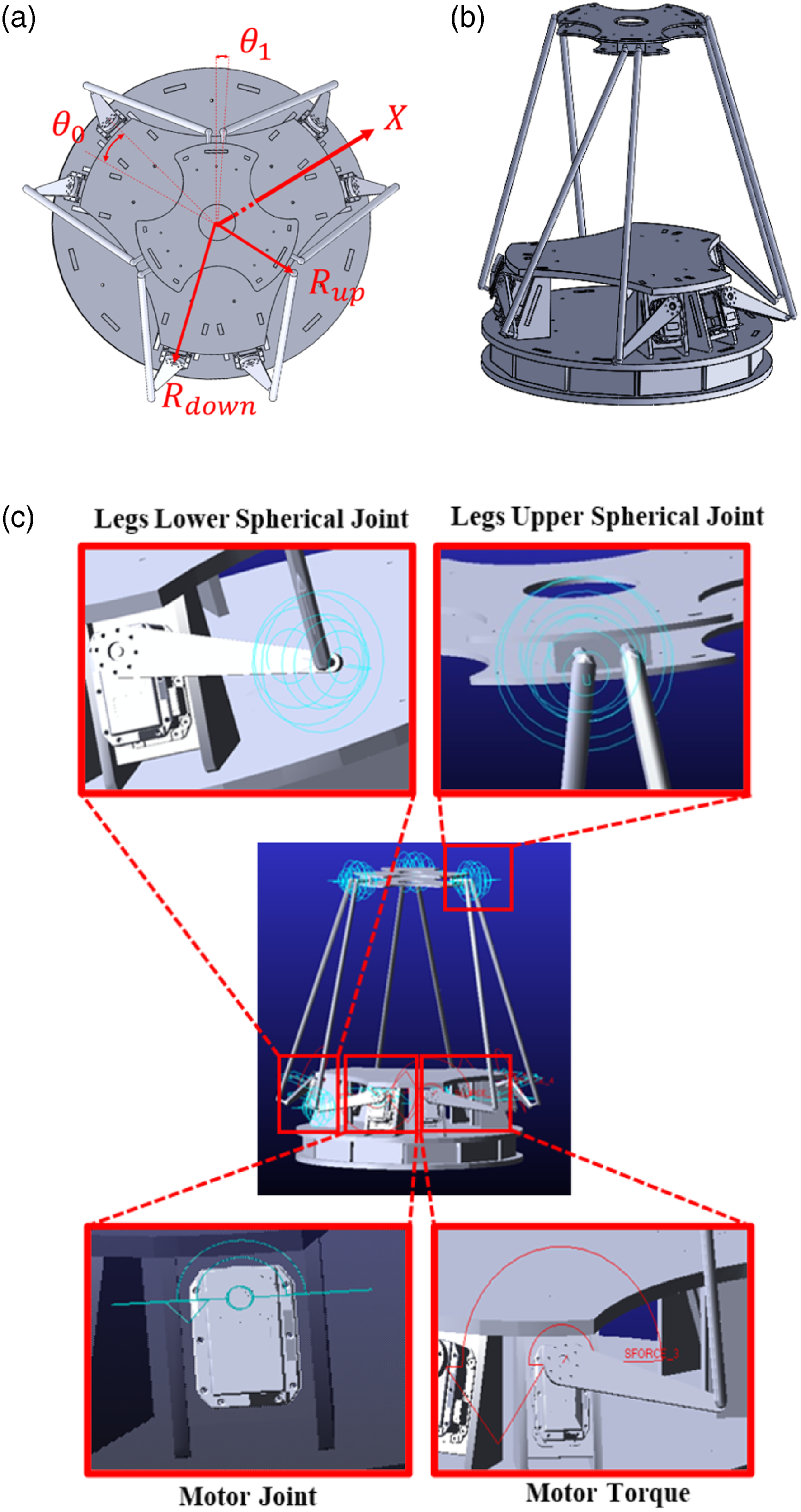
3. Controller design
According to the fact that the designed dynamical system in ADAMS consists of nonlinear parameters of an actual system, it is definitely a nonlinear Stewart platform. Hence, to control these kinds of systems, the proposed controller needs to be capable of reducing the tracking errors in the presence of nonlinearities (Åström and Hägglund, 1995). In addition to robustness, optimization of the input signals in parallel manipulators to achieve an efficient performance is a challenge. The issue needs to be addressed in the controller design process. Therefore, a linear quadratic integral (LQI) optimal controller is an appropriate option to control the nonlinear system effectively.
3.1. State-space equations
The state space and dynamic equations of the Stewart robot can be formulated as follows

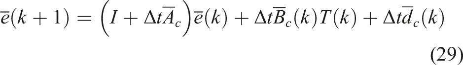

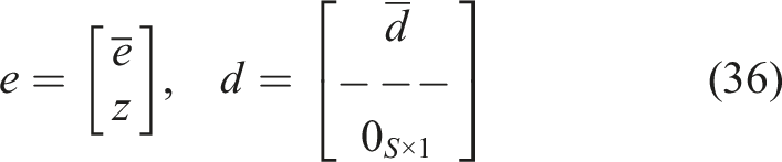
Therefore, the resulted dynamic error of the system which appears after adding the integral states can be written as

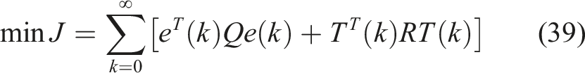

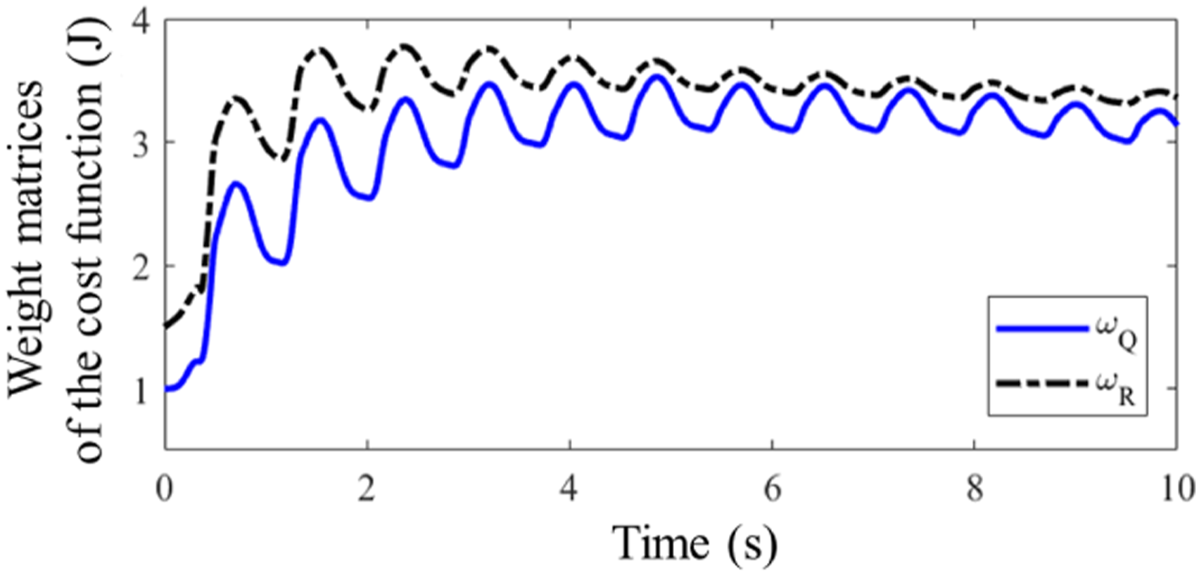
Matrices Q and R are weight matrices aiming to minimize all the states’ error and the control signals. And the weighting matrices are formulated by ω Q > 0 and ω R > 0.
The resultant optimal control problem in equations (39) and (40) is solved by using a linear quadratic regulator (LQR). The goal is to stabilize feedback gains through the assumption (Tajdari and Roncoli, 2021), whereas stability and detectability criteria of Lewis et al. (2012) in chapter 2 should be satisfied by the original system in equation (35).
3.2. Stability and detectability
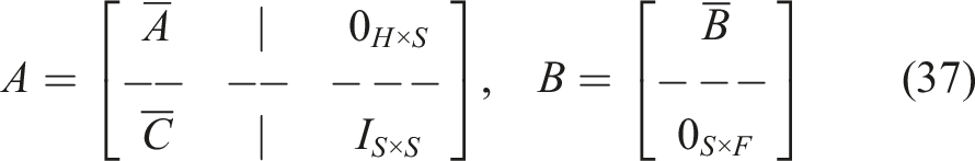
Stabilizability and detectability of the system in equation (35) are studied by conductin the Hautus test (Williams and Lawrence, 2007). Referring to Williams and Lawrence (2007), B is assumed to include more linearly independent columns in comparison with the number of unstable (λ ≤ 0) modes, to be able to guarantee stability of the pair (A, B). Depending on the system topology, matrix 
Now, the detectability of the system can be addressed in the pair (A, C
T
QC); regarding Hespanha (2009), because Q > 0, this is essentially equal to study of the detectability of the pair (A, C). In the existing problem, the Hautus test condition is validated as follows in the situation that C contains at least one nonzero element in each column according to the marginally stable mode (λ = 0). By considering that, in all the discussed scenarios, the system is assumed to be observable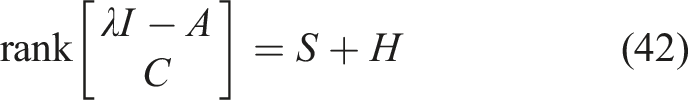
3.3. Controller design and anti-windup
To solve the LQI problem, a linear feedback control law is proposed as follows


resulted K in equation (44) as optimal gain, and the algebraic Riccati equation equation (45) is investigated in Navvabi and Markazi (2019). Moreover, regarding practical implementation, the gain K is divided into two sections as follows

The final control law equation (47) is substantially effective for practical implementations because the computational effort manipulated by the feedback gains K P and K I presents considerably lower values.
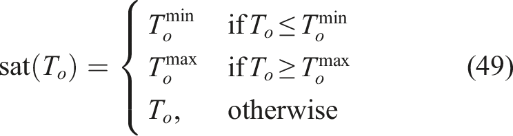
In practical applications, achieving the exact values of the desired states may not be always possible due to uncertainties such as input saturation problem. Hence, it is prerequisite to use an anti-windup scheme within the proposed controller. The proposed scheme in Åström and Rundqwist (1989) is used in this study. In the case of this research, the scheme modifies the integral part of the dynamic controller equation (47) as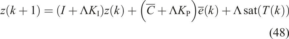
Therefore, the ultimate equations of the dynamic regulator are equations (47) and (48), which are practically effective and robust. Because it may affect the offline computation of the feedback gains KP, KI, in solving equations (44) and (45) (where B is time-varying), online calculations are restricted to solving equations (47) and (48).
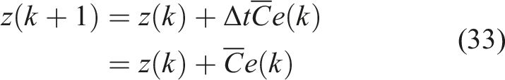
It should be noted that while T(k) does not exceed the saturation boundaries, the dynamics equation (48) is reduced to equation (33). Also, the numerical experiments clarify that the selection of different nominal values of T has explicitly no influence on the controller execution. It can be determined by the ability of the integral controller to dismiss the disturbances (Åström and Hägglund, 1995).
3.4. Anti-windup stability analysis in the closed-loop system
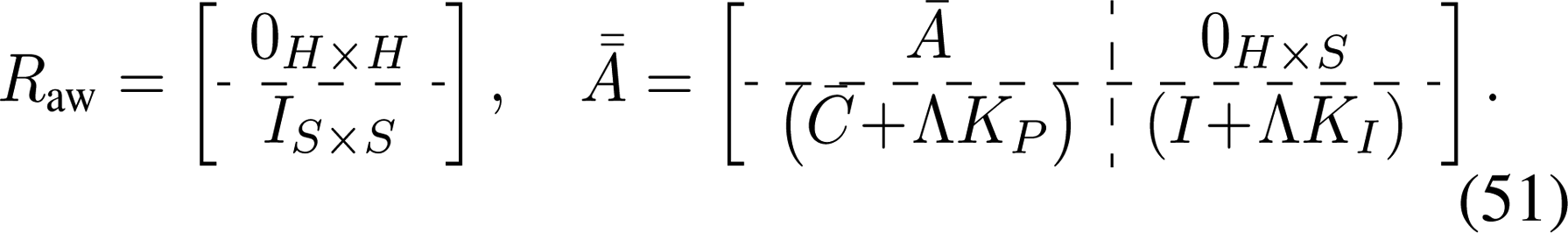
An essential constraint for the stability of the closed-loop system with the anti-windup scheme which conveys matrix Λ must be properly selected so that I +ΛK
I
has stable eigenvalues
To demonstrate the closed-loop system stability for the case that the inputs are saturated, equation (35) is reformulated as
Referring to da Silva Jr and Tarbouriech (2006), if a symmetric positive definite matrix is found as 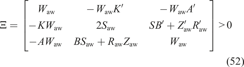

3.5. Sensitivity analysis
To test the suggested strategy, the dynamic compensator equations (47) and (48) is applied to the nonlinear ADAMS model, whereas
Regarding investigating the sensitivity of the controller to select parameters w
Q
, w
R
, and 
Figure 3(a) shows how the achieved Numerical analysis. (a) Sensitivity analysis based on 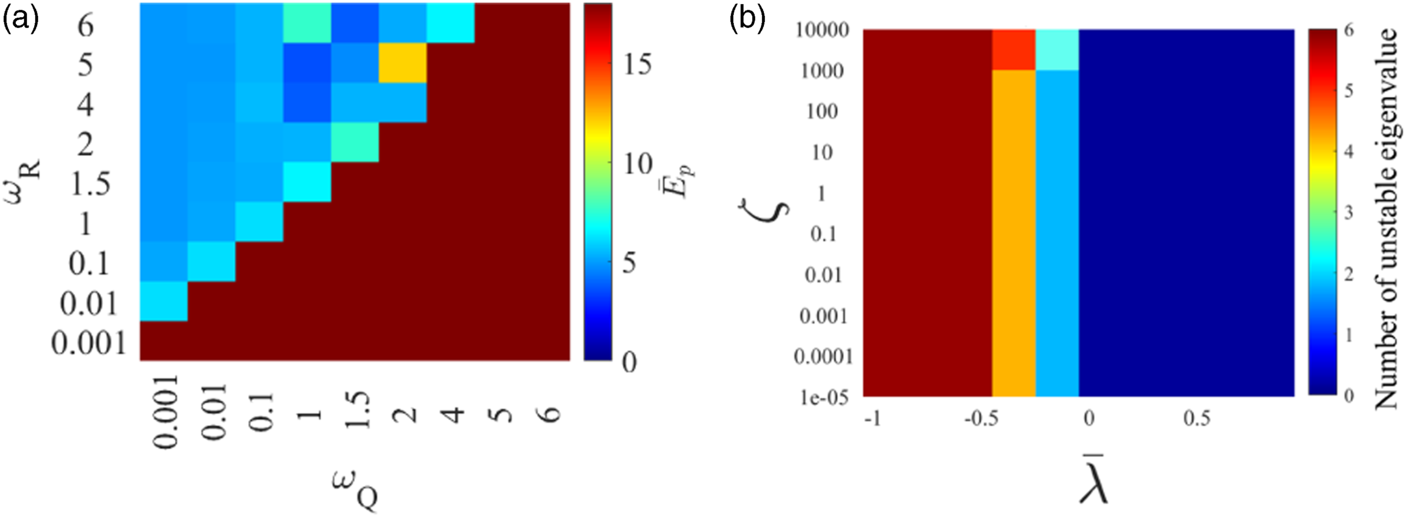
Although the reasonable results (with acceptable
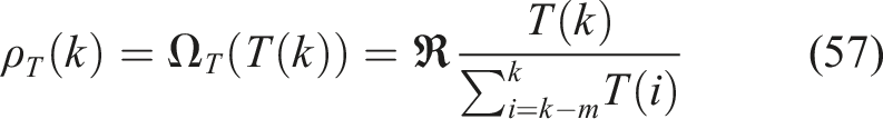
Because the parameters of dynamic equations in equation (27) are time variants,
The functions are selected based on Tarvirdizadeh et al. (2018). Therefore, in this problem, density functions of error state and torques are appropriate functions to describe the changes, which are elaborated as follows Designed artificial neural network estimator structure.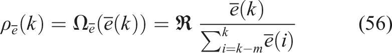
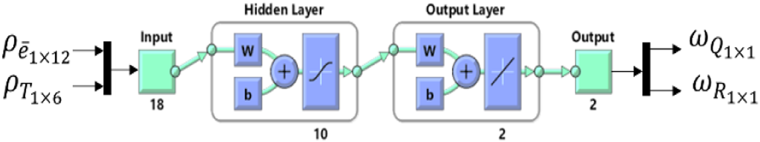
To design the estimator, the dataset is randomly divided into two subsets: the training and the testing data subsets. The first data subset is used to develop and fine-tune the estimator. Afterward, the second data subset is used to assess the estimator performance, which does not affect the training data subset. Thus, the first data subset, which contains 70% of the master dataset, is considered for training and the remaining of 30% is used to validate the obtained model. Figure 5 shows the closed-loop optimal feedback control diagram of the proposed system, where the ANN estimator based on the error states and the torques’ values, updates the controller gains of w
Q
and w
R
in each time step. Closed-loop control diagram.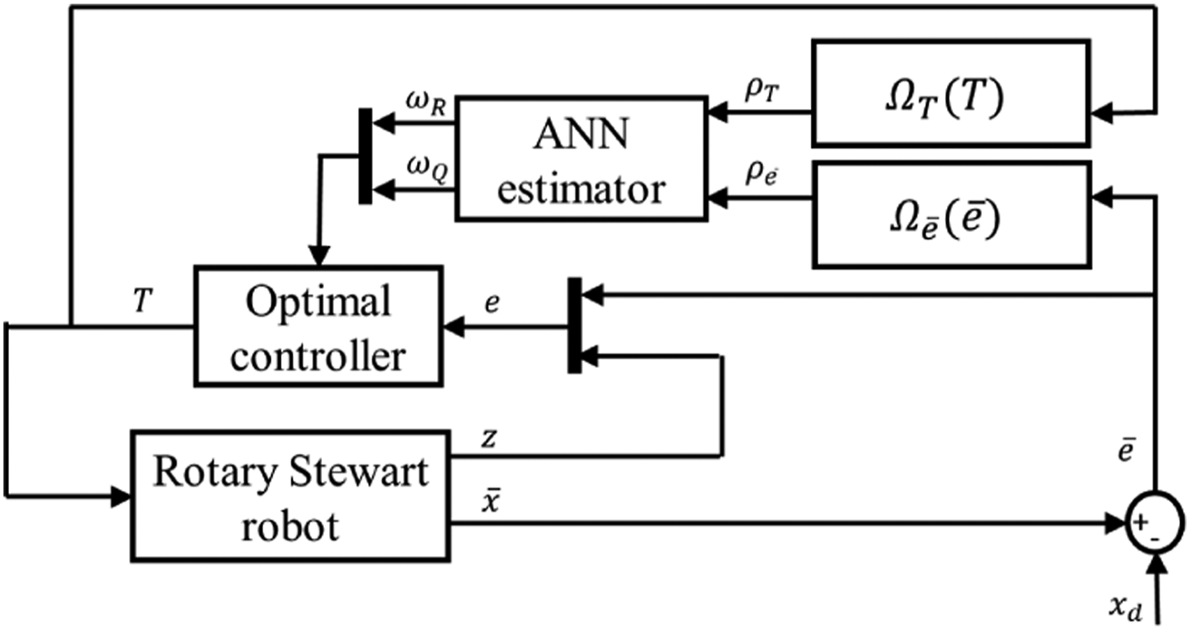
4. Experiment setup
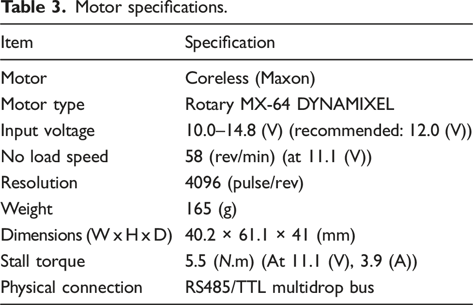
To evaluate the controller in a real nonlinear system with natural disturbances, the introduced robot in Figure 2 was fabricated. As Figure 6 depicts, 6 servo motors of mx-64 are used as torque manipulators and are controlled directly with MATLAB through USB2Dynamixel (Robotis, (2019b). These motors are selected due to having incremental encoder and torque meter with acceptable resolution. Moreover, the stall torque for these motors is 5.5 N.m, which is relatively high. The specifications of the motor extracted from Robotis (2019a) are reported in Table 3. Moreover, to measure the end effector position and angles Fabricated rotary parallel robot. Motor specifications.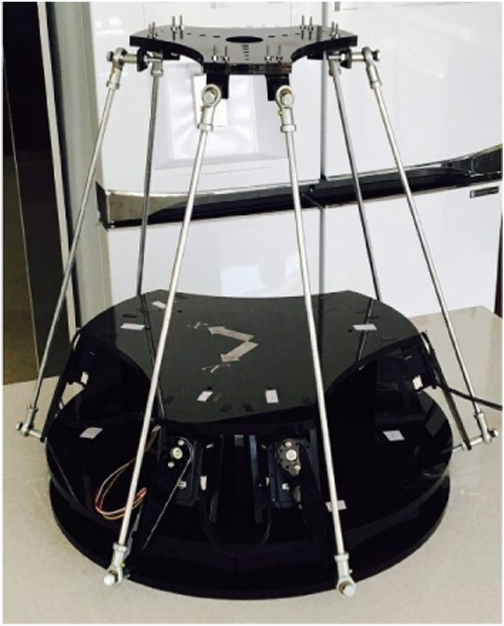
5. Results
5.1. Simulation results
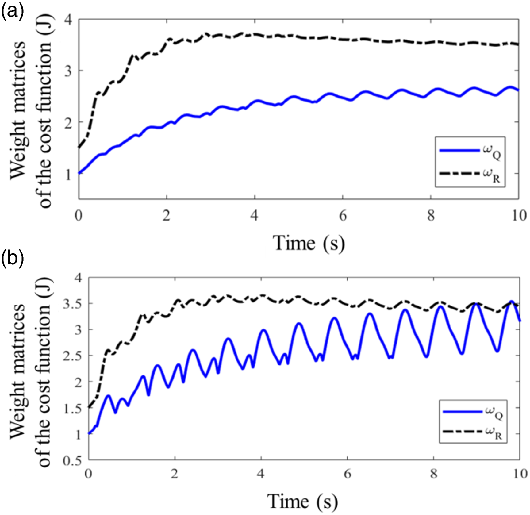
The simulation results are generated by implementing the proposed controller of equations (47) and (48) on the ADAMS model in Figure 2(c), where Online estimated of w
Q
and w
R
for the ADAMS model controlled case. (a) Constant mass value of m = 4 kg. (b) The time-varying mass value in equation (60).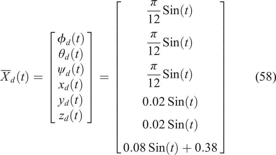
Moreover, the implemented torques (T
i
in equation (16)) on the system for the three control scenarios are shown in Figure 9. Based on Figure 9(a), the controller I practically generates no control signals due to no tracking actions of the desired values in Figure 7(a). Comparing the torques in Figure 9(c) with Figure 9(e), the anti-windup integral controller with the ANN estimator offers less saturated (especially for the upper boundary saturation) and smaller torque values in comparison to the anti-windup integral controller without the estimator. It is due to less tracking error, and consequently less integral states’ values, which are achieved by the anti-windup integral controller with the ANN estimator, rather than the integral controller without the estimator. Furthermore, the torque analysis is used to choose the electromotor discussed in the Experiment Setup section. Motor torques for the ADAMS model controlled case. Controller I: (a) constant mass value of m = 4 kg and (b) time-varying mass value in equation (60). Controller II: (c) constant mass value of m = 4 kg and (d) time-varying mass value in equation (60). Controller III: (e) constant mass value of m = 4 kg and (f) time-varying mass value in equation (60).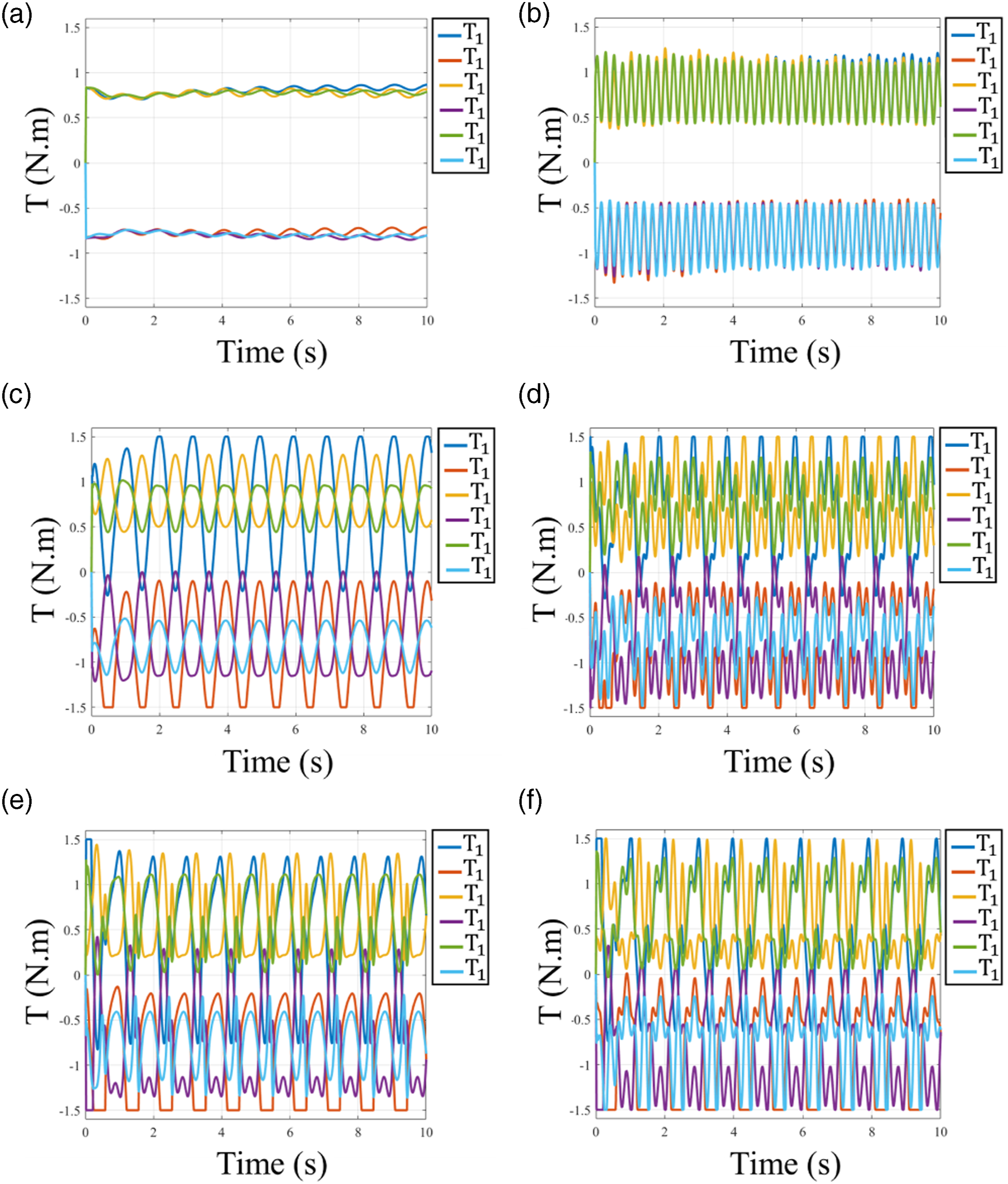
Envisioning the motor torque saturation, it is worth investigating the robustness of the controllers with respect to different kinds of constant and dynamic time-variant load torque with high probability of motor torque saturation. Accordingly, the effect is numerically studied through the following experiments.
Accumulative absolute percentage error (E ac ) and the total saturation time report (t sat ).
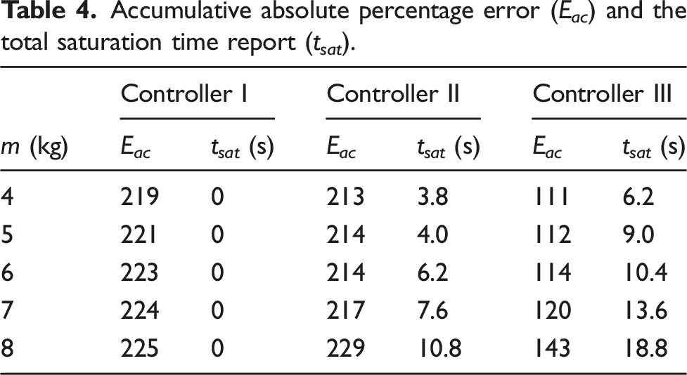
Time-variant load torque investigation: Accordingly, an experiment is arranged where the mass of the end effector is time-varying as follows
5.2. Experiment results
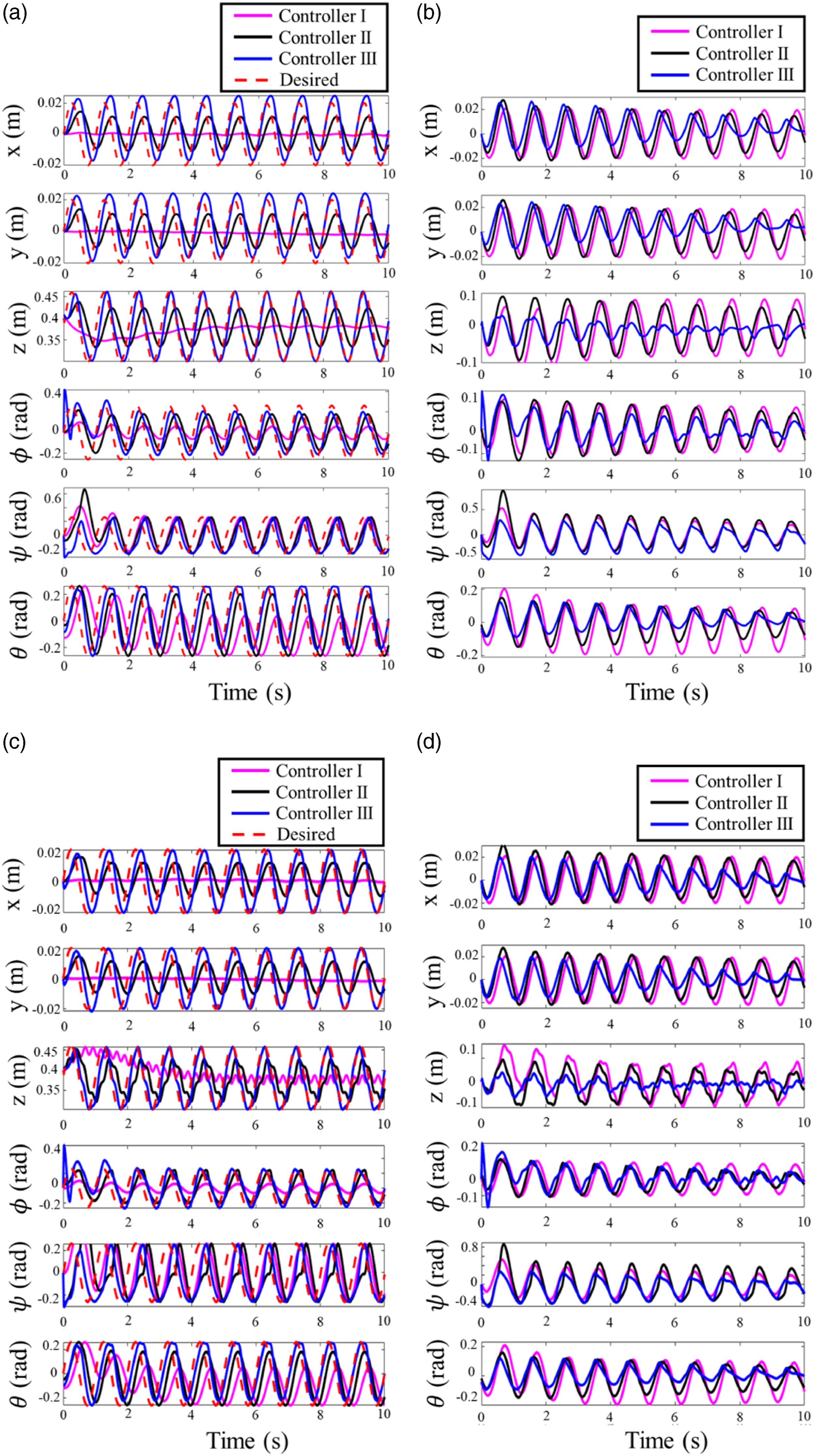
To validate and investigate the reliability of the proposed controller in the presence of real disturbances and uncertainties, the controller is implemented on the robot introduced in the Experiment Setup section. To have a comparison with the simulation output, the same desired values in equation (58) are used. All the other control parameters and initial conditions are considered the same as the Simulation results section. Performances of the controllers for the main states are depicted in Figure 10(a). Comparing the results of the three controllers in the figure gives the same conclusion as the previous section because the rate of the error rejection for the anti-windup integral controller with the ANN estimator (controller III) is considerably higher than the other two controllers. However, more overshoot is observed in the beginning of the test. The overshoot happened regarding the unexpected actuators’ lag and unidentified dynamical parameters. This issue is also detectable in the trajectories of the estimated w
Q
and w
R
in Figure 11 as they have high fluctuating behavior in the beginning of the test, whereas they are converging by the time to specific values. In addition, the ANN estimator is supposed to present the parameters in which the tracking errors are minimized. Only for the control strategy with the estimator, the tracking errors drawn in Figure 10(b) are decreasing by the time due to w
Q
and w
R
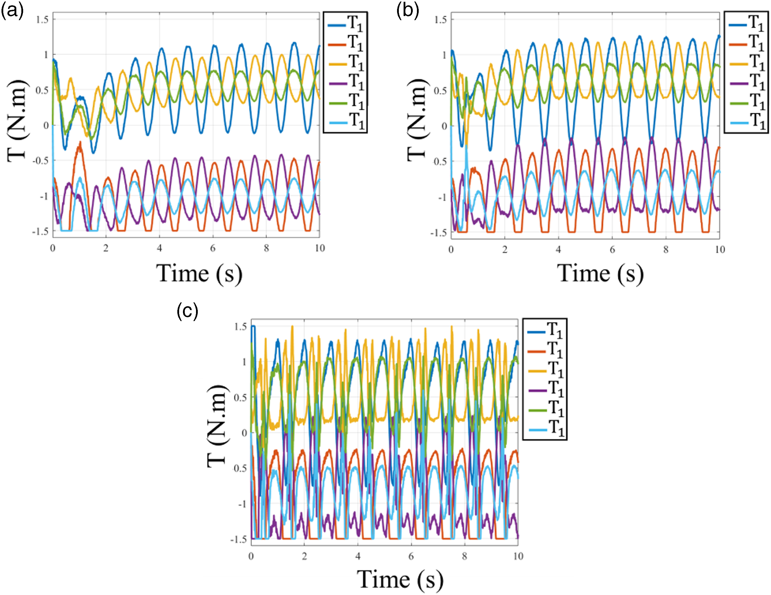
identification. This infers well-practical performance of the estimator. Comparing the torque diagrams in Figure 12 illustrates that outputs of the controller with the ANN estimator (controller III) in Figure 12(c) are saturated in more time span comparing to Figures 12(a) and (b), although the results show zero-converging error for the controller. This implies a logic cooperation between the estimator and the anti-windup scheme in equation (48), resulted from little sensitivity of the parameters choice to performance of the controller. Controlled case performance through the fabricated robot. (a) Main states Online estimated of w
Q
and w
R
for the fabricated robot controlled case. Motor torques for the fabricated robot controlled case. (a) Controller I. (b) Controller II. (c) Controller III.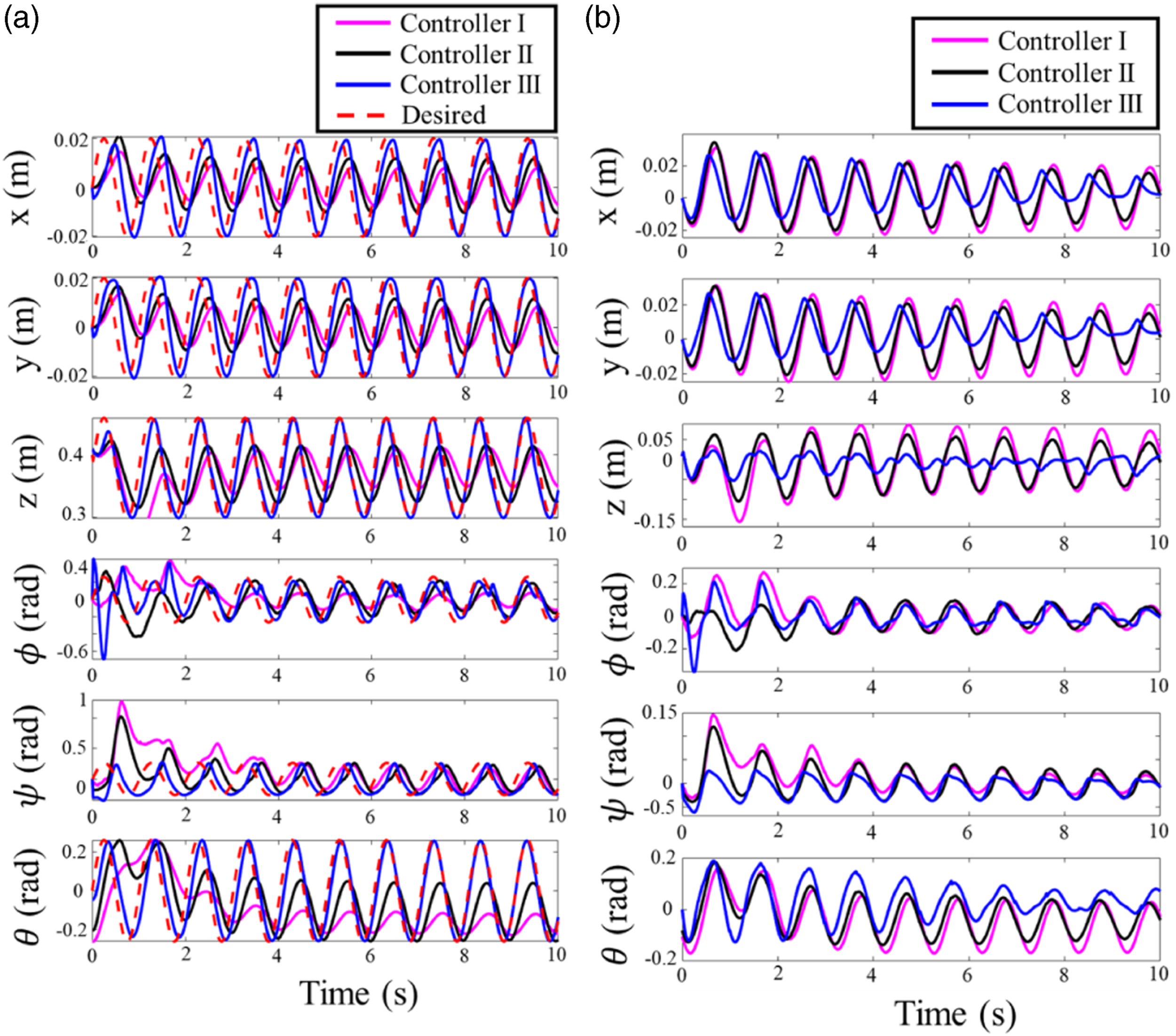
6. Conclusion
In this article, an innovative control methodology for a Stewart platform parallel robot with rotary actuators was investigated. The equations of motion for the system were derived and a 3D model of the system was also implemented in ADAMS. In addition, the analyses of the kinematic, dynamic, and control of the robot were investigated based on the obtained nonlinear model. To attain a desired amount of the end effector tracking error, the gain tuning LQI controller. The robustness and insensitivity of the parameter choices, besides the adaptive component, that is, the ANN estimator, made practical implementation easier, without the necessity of lengthy and costly measurements of the dynamic parameters. Finally, the simulation results revealed that the optimal LQI controller with intelligent estimator was able to control the dynamic of the system and eliminate the tracking error 45% more than the other compared controllers, averagely, considering the existence of the realistic dynamic forces and saturation in the ADAMS model. Also, the methodology was evaluated by the fabricated rotary Stewart robot to investigate the robustness of the controller with respect to the dynamic parameters, uncertainty, and realistic noise. Future developments include the optimal dimension design subject to the dynamic of the system and the study of the controller sensitivity regarding the dimension of the robot and dynamic parameters. In addition, the fabrication of a faster and smaller robot integrated with a time-delay optimal controller is another topic for the future studies to be easily adaptable to other practical cooperative robots.
Footnotes
Declaration of conflicting interests
The author(s) declared no potential conflicts of interest with respect to the research, authorship, and/or publication of this article.
Funding
The author(s) received no financial support for the research, authorship, and/or publication of this article.