Sage Journals: Discover world-class research

Abstract

This article presents the application of phase space topology and time-domain statistical features for rolling element bearing diagnostics in rotating machines under variable operating conditions. The results indicate very promising performance in identifying various faults with virtually perfect accuracy, recall, and precision. A comparison with the envelope analysis method is performed to show the superior performance of the proposed approach. In addition, the results demonstrate an outstanding prediction rate for the fault diameter of bearing defects.

Keywords

Rolling element bearings bearing diagnostics phase space topology machine learning feature extraction

1. Introduction

Diagnostics of rolling element bearings has gained considerable interest because of the extensive use of these elements in rotating machinery systems and because their failure is one of the most common causes of machinery breakdown. Predicting the potential breakdown of a machine would be invaluable in preventing catastrophic failures and loss of production. Accurate predictions can also improve safety and reduce repair costs in most industries (Randall, 2011).

Condition-based maintenance or predictive maintenance is one of the most common maintenance strategies and is based on performing an online assessment of machines while operating. It also provides information about the machine’s health condition and any potential failures. This type of maintenance strategy requires techniques that continuously monitor the performance of the machine and provide knowledge about the status of the system, including any faults, their locations, and severity levels.

To this end, rolling element bearings are traditionally diagnosed using various time-domain techniques (Du et al., 2017; Honarvar and Martin, 1997; Prieto et al., 2013; Samanta and Al-Balushi, 2003; Sreejith et al., 2008) and various frequency-domain techniques, such as fast Fourier transform (FFT) (Nikolaou and Antoniadis, 2002; Rai and Mohanty, 2007; Seryasat et al., 2010; Shibata et al., 2000), short-time Fourier transform (STFT) (Cocconcelli et al., 2012; Gao et al., 2015; Peng and Chu, 2004), discrete wavelet transform (DWT) (Kankar et al., 2011a, 2011b; Konar and Chattopadhyay, 2011; Patil et al., 2016; Prabhakar et al., 2002), envelope analysis (Ho and Randall, 2000; Ming et al., 2011; Patel et al., 2012; Peter et al., 2001; Randall and Antoni, 2011; Rubini and Meneghetti, 2001; Yang et al., 2007b), and empirical mode decomposition (EMD) (Ali et al., 2015; Lei et al., 2013; Zhang and Zhou, 2013; Zhang et al., 2015; Zhao et al., 2013). The FFT does not work well when analyzing nonstationary signals. The STFT provides constant resolution for all frequencies because it uses the same window for the entire signal, and a time–frequency resolution trade-off is necessary. The DWT involves selecting the base function and particular frequency bands with defect information. Envelope analysis methods necessitate determining the central frequency and the bandwidth, and an improper selection of these parameters can affect the analysis significantly. EMD requires selecting a suitable decomposition level and its intrinsic mode function. More recently, fault detection and diagnosis in bearings have been widely studied using artificial intelligence (Borghesani et al., 2013; Gan et al., 2016; Gryllias and Antoniadis, 2012; Jung and Koh, 2015; Pandya et al., 2013; Peng et al., 2005; Xiang et al., 2015; Yang et al., 2005).

For many applications, it is desirable to develop robust algorithms that can provide rich information to identify faults and their severity quickly and in an automated fashion. The key to robust and accurate diagnostics is being able to extract suitable indicators from the raw data that reveal relevant and informative patterns about the intrinsic dynamics of the system.

In our previous work, we have performed various investigations to develop robust techniques to diagnose bearings. In Kappaganthu and Nataraj (2011a, 2011b), we have applied conventional methods such as FFT, envelope spectrum, and DWT over a span of rotational speeds. Accelerometer data were used to extract features to diagnose bearings with inner race (IR), outer race (OR), and ball (B) defects. Mutual information was then used as a ranking technique, and the optimal feature subset corresponding to the highest classification accuracy was determined. Although all these techniques can extract detailed information from the system response, they depend on expert knowledge and require to be carefully designed and adapted to a particular problem. Moreover, these methods do not consider the fundamental nonlinear physics of the system, which could have valuable insights, as was shown in our work Kwuimy et al. (2018) and Maraini and Nataraj (2018). The present study is a continuation of our development of a family of methods based on phase space characterizations (Mohamad and Nataraj, 2017; Mohamad et al., 2018a, 2018b, 2018c, 2019; Samadani et al., 2013, 2016).

In our previous studies (Mohamad et al., 2018d), we have applied a novel feature extraction technique called phase space topology (PST) to classify various bearing conditions under variable speeds using vibrational data from proximity probes. By contrast, the current study applies PST using accelerometer data in consideration of the fact that accelerometers are extensively used for bearing diagnostics. We also analyzed various bearing conditions with varying severity under variable operating conditions such as speed and load. This difference makes the diagnostic problem more challenging and closer to realistic scenarios.

The developed method is based on quantitative characterization of the topology of the bearing vibrational signal. As will be shown, not only does the proposed method show superior performance over standard envelope analysis methods but also it can also be applied to diverse dynamical systems with minimal requirements for a priori knowledge about the nature of the system or adaptation to a specific problem. It should be acknowledged that several studies based on the phase space of the system in the field of structural health monitoring (SHM) have been reported in the literature (George et al., 2018; Nichols, 2003; Nie et al., 2012; Todd et al., 2001; Torkamani et al., 2012). Although they are superficially similar to our method, there are substantial differences. Most of these methods excite the structure with a chaotic input to extract a single feature and target SHM applications. Furthermore, the PST method described below presents original concepts such as kernel density–based features, density approximation, and orthogonal basis functions as a feature extraction technique.

The proposed method in this study is applied to the vibration signals of two bearings as measured by accelerometers, which are conventionally used as vibration sensors for bearing analysis and fault diagnostics (Randall and Antoni, 2011; Samanta and Al-Balushi, 2003; Zhou et al., 2007). The most common failure modes in bearings are cracks on the surfaces of the IR, OR, and roller components. Therefore, four different drive end (DE) bearing conditions are considered, including a healthy bearing (H), and bearings with IR, OR, and B defects.

The rest of this article is organized as follows. In Section 2, the experimental setup and measurement of data are introduced. Section 3 summarizes the mathematical details of the proposed feature extraction method. Section 4 discusses the results of fault identification along with a comparison with the envelope analysis method. In Section 5, fault severity analysis is performed. Finally, Section 6 concludes and summarizes the study.

2. Experimental setup

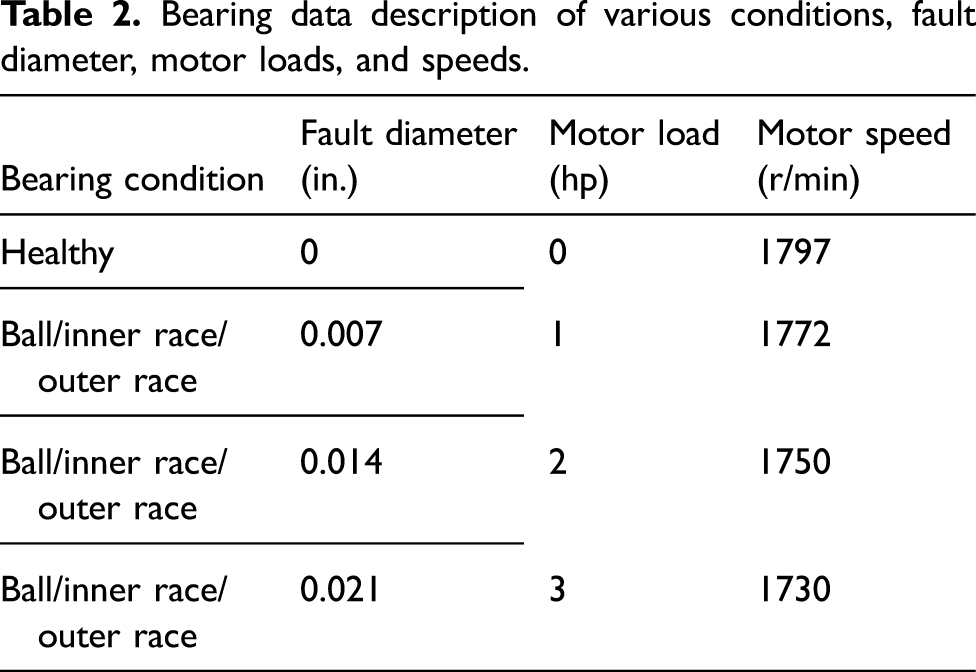
The proposed approach in this study was implemented on data collected from motor bearings provided by Case Western Reserve University (Loparo, 2003; Smith and Randall, 2015). The experimental setup and its schematic diagram that are used in the study are shown in Figure 1. The bearing experimental setup consists of a 2-horsepower (hp) motor with a torque transducer/encoder and a dynamometer. The dynamometer was used to apply various loads on the electric motor. For this study, four motor loads of 0–3 hp (motor speeds of 1797–1720 r/min) were considered. SKF deep groove ball bearings were used for both DE and fan end (FE) bearings. The DE and FE bearing geometries (measured in inches) are presented in Table 1.

Figure 1.

(a) Bearing experimental test (Loparo, 2003). (b) Schematic diagram of the test rig.

Table 1.

Bearing information (in.) (Loparo, 2003).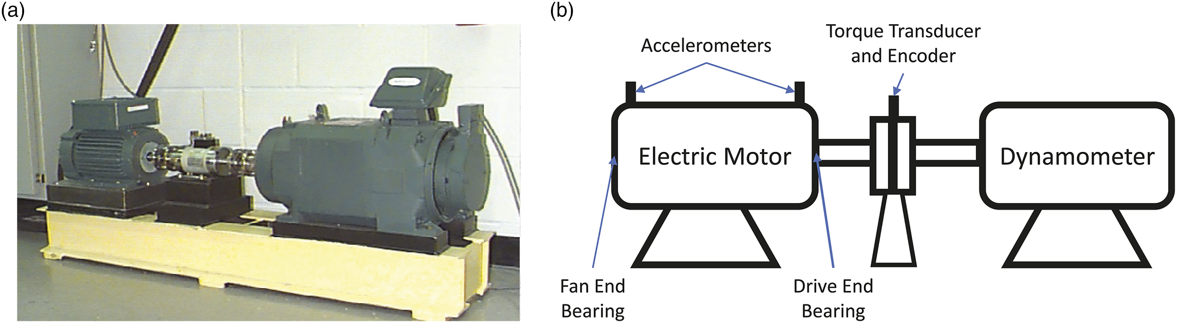

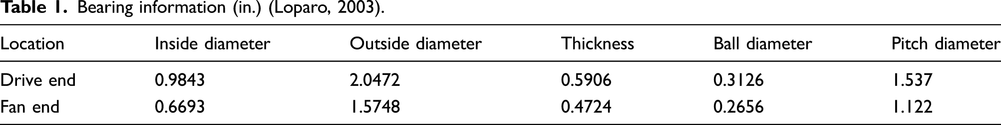
Location	Inside diameter	Outside diameter	Thickness	Ball diameter	Pitch diameter
Drive end	0.9843	2.0472	0.5906	0.3126	1.537
Fan end	0.6693	1.5748	0.4724	0.2656	1.122

Multiple test DE bearings with different health conditions including one healthy bearing (H) and three defective bearings with B defect, IR defect, and OR defect were investigated. DE bearing with IR, OR, and B defects were seeded with single-point faults with diameters of 0.007, 0.014, and 0.021 in. and a depth of 0.011 in. using electro-discharge machining. For OR defective bearings, the faults were seeded at the 6 O’clock position. The FE bearing condition was healthy for all conducted tests. Table 2 summarizes the collected data and the operating conditions. It should be clarified that experiments for various bearing conditions and fault diameters were conducted for each individual motor operating condition, that is for each load and its corresponding speed that are listed in the table.

Table 2.

Bearing data description of various conditions, fault diameter, motor loads, and speeds.

Bearing condition	Fault diameter (in.)	Motor load (hp)	Motor speed (r/min)
Healthy	0	0	1797
Ball/inner race/outer race	0.007	1	1772
Ball/inner race/outer race	0.014	2	1750
Ball/inner race/outer race	0.021	3	1730

The vibration signals were recorded using accelerometers installed on the DE and FE bearing housings at the 12 O’clock position. The signal was recorded for approximately 20 s for healthy and 10 s for defective bearing conditions. The sampling rate of the measured vibration data was 12,000 Hz. Selected samples of vibration data captured by the accelerometers under zero motor load and for 0.25 s are shown in Figure 2. Note that all time responses of the defective bearings shown in Figure 2 have a fault diameter of 0.007 in. and a fault depth of 0.011 in.

Figure 2.

Sample response of the system. (a) Healthy bearings. (b) DE bearing with ball defect. (c) DE bearing with inner race defect. (d) DE bearing with outer race defect. DE: drive end.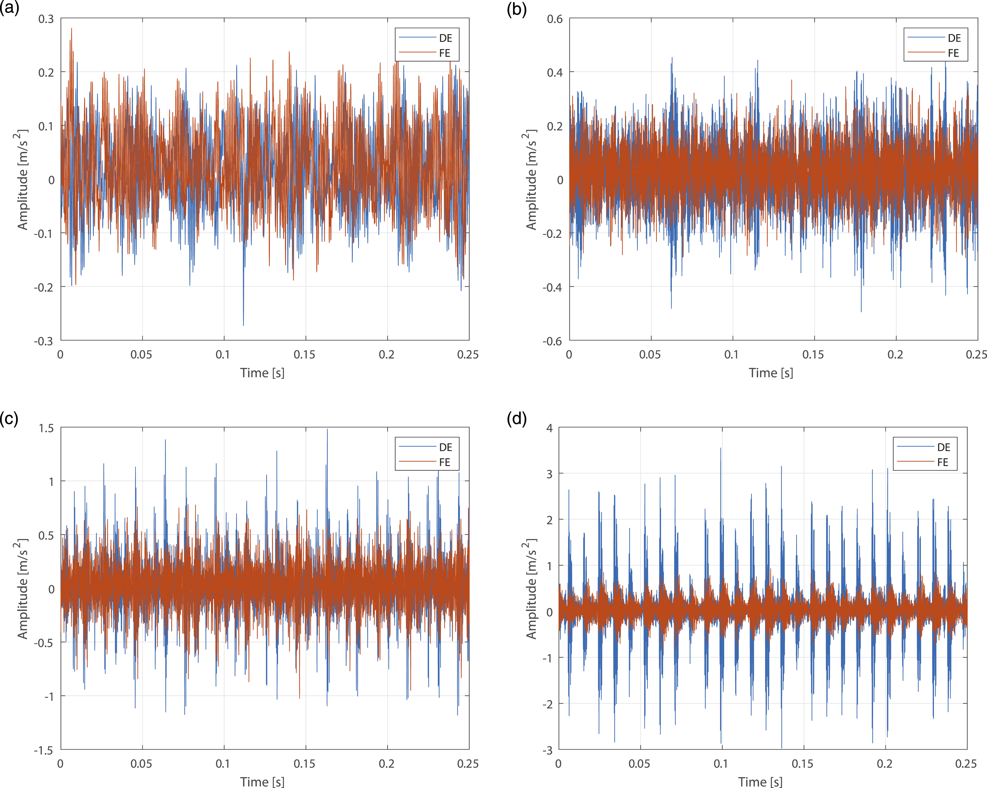

3. Methodology

An overview of the fault detection method used in this study is summarized in Figure 3 and is as follows. First, acceleration data of the DE and FE bearings were collected for healthy FE and various DE bearing conditions operating under variable motor loads and rotational speeds. Four DE bearing conditions were studied including healthy bearing (H) and bearings with IR, OR, and B defects. The vibration data were then divided into multiple segments of one-second time periods. For each segment, two sets of features were extracted using the PST method and conventional statistical time-domain features. A linear support vector machine (SVM) was built to identify the DE bearing condition, that is H, B, IR, and OR. In the case of a bearing fault, an additional SVM was then built for each individual fault to estimate the fault severity (i.e. 0.007, 0.014, or 0.021 in.).

Figure 3.

An overview of the bearing diagnostics method.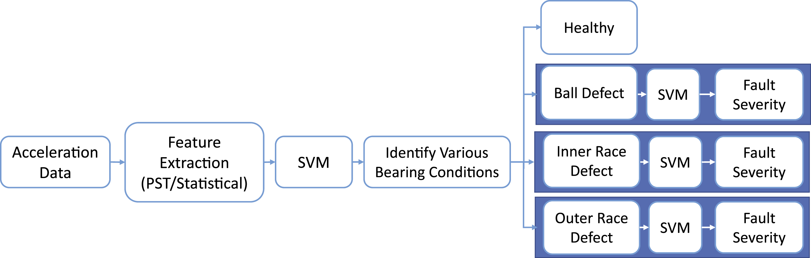

3.1. Phase space topology

The PST method assumes that useful and relevant information is contained in the nonlinear response of dynamic systems. The phase space is a prevalent concept in nonlinear dynamics, in which a trajectory is a visual representation of the traced path of possible states of the system evolving over time (Nolte, 2010). Each kind of system response has a unique phase space trajectory. For example, a periodic response with a single frequency has a single closed loop, whereas multi-periodic and quasi-periodic responses have multiple loop trajectories. This indicates that the phase space trajectory can be used to characterize the nature of the system in a qualitative fashion as is done traditionally in nonlinear dynamics. The method of PST is, however, based on characterizing the PST with quantitative measures by constructing the density distribution for each axis of the phase space.

To estimate the density distribution for each phase space axis, the kernel density estimation technique was implemented as follows. Let X = (x₁, x₂, …, x_n) be a set of n sample data that are independent and identically distributed with an unknown density function Ψ. The kernel density estimator, 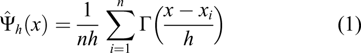${\hat{Ψ}}_{h} (x)$ , can estimate the shape of this function, where the symbol ^ indicates that it is an estimate and the parameter h is the bandwidth parameter or the smoothing parameter

{\hat{Ψ}}_{h} (x) = \frac{1}{n h} \sum_{i = 1}^{n} Γ (\frac{x - x_{i}}{h})

(1)where Γ(·) denotes the kernel function, which satisfies the following two conditions

\int_{- \infty}^{\infty} Γ (u) d u = 1

(2)

Γ (- u) = Γ (u) \forall u

(3)

There are a variety of kernel functions such as uniform, triangular, biweight, triweight, Epanechnikov, and Gaussian. The Gaussian density function was used because of its conventional and convenient mathematical properties and is defined as follows

Γ (u) = \frac{1}{\sqrt{2 π}} e^{- (1 / 2) u^{2}}

(4)

The kernel density estimator’s performance depends primarily on the bandwidth parameter h. Small values of h will cause the density estimate to be undersmoothed, whereas large values will lead to an oversmooth density estimate. The optimal value for the bandwidth can be calculated using Silverman’s rule of thumb (Silverman, 2018) for Gaussian kernel functions as follows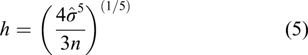

h = {(\frac{4 {\hat{σ}}^{5}}{3 n})}^{(1 / 5)}

(5)where

\hat{σ}

is the standard deviation (SD) of the samples and n is the number of samples. It is important to have the number of samples n as high as possible for estimating the density distribution. However, increasing n will also increase the computation cost.

After constructing the density distribution for each phase space variable, the PST method is used to extract kernel density–based features from these distributions. To illustrate, let us consider the following elementary example of a multi-harmonic response in two-dimensional space

x_{1} = \sin (π ω_{1} t) + \sin (π ω_{2} t)

(6)

x_{2} = π ω_{1} \cos (π ω_{1} t) + π ω_{2} \cos (π ω_{2} t)

(7)where x₂ = ẋ₁, ω₁ = 10 Hz, and ω₂ = 20 Hz. The phase space plane for the given system is presented in Figure 4(a).

Figure 4.

An example of a multi-harmonic response. (a) Phase plane. (b) Density distribution of x₁. (c) Density distribution of x₂. (d) Phase plane with the location of the corresponding distribution peaks.

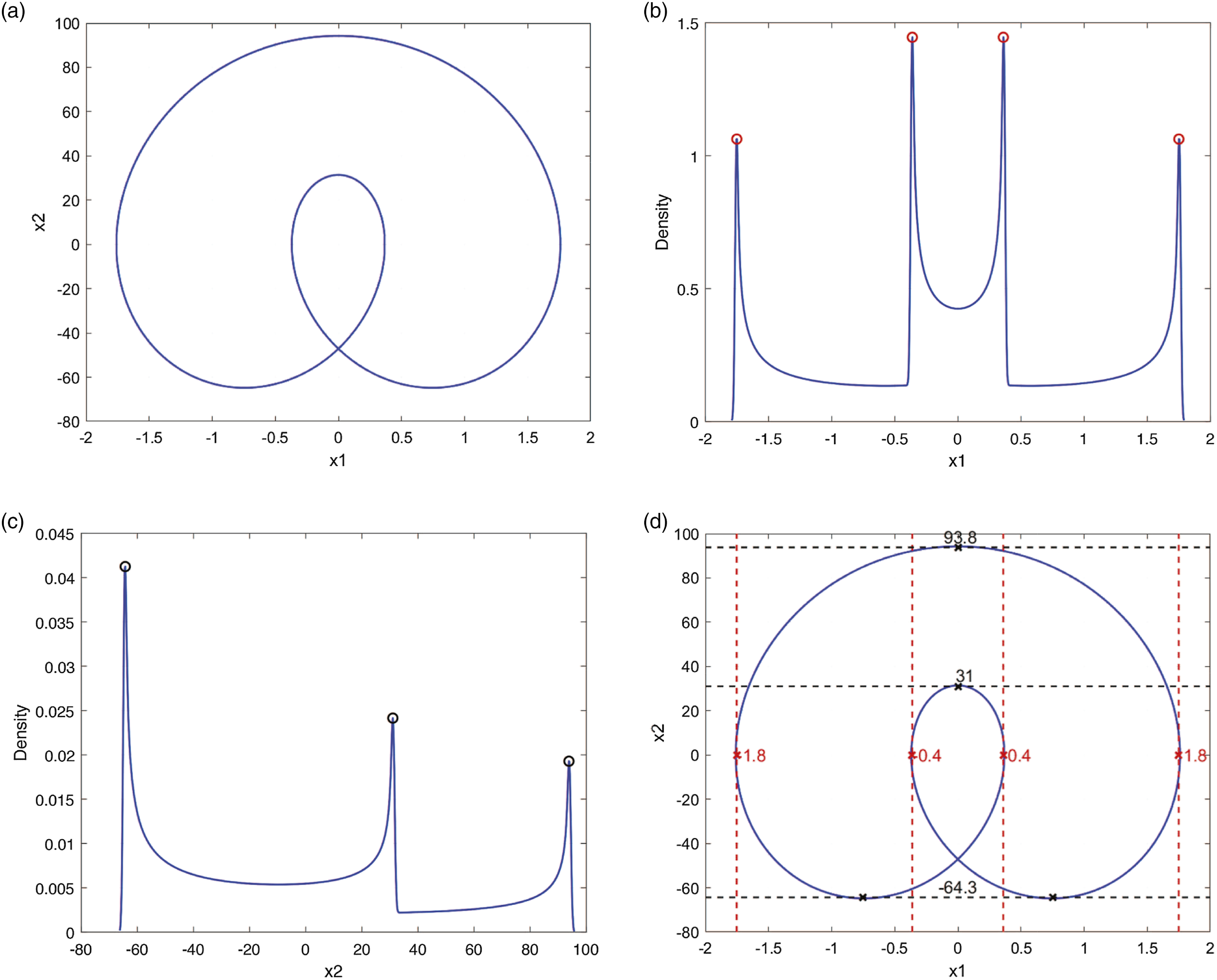
In the phase plane, multiple loops are caused by the multi-harmonic response. The corresponding density distribution of the x₁ variable is estimated and shown in Figure 4(b). As can be seen, four sharp peaks are caused by the higher concentration of points in the corresponding areas in the phase plane plot shown in Figure 4(d). In fact, the ends of the loop along the vertical axis in the phase plot, which we call the “returning points,” are the areas in which the system spends more time. Note the symmetry of the density distribution and the peaks which are due to the symmetry of the phase plane around the zero of x₁. Similarly, the density distribution for the x₂ variable of the phase plane is shown in Figure 4(c). Three unique peaks correspond to the returning points along the horizontal axis in the phase plane and are marked in Figure 4(d) to emphasize the point.

We originally used the peak properties of the estimated density distribution, including the location, height, and sharpness of the peaks as characteristics to describe the system response. Although visualization of the phase space trajectory is not possible for dimensions higher than three, the method is still applicable. This is because the computations are performed individually and independently for each state of the system.

The peak properties of the density distribution alone are not enough to fully describe the behavior of the system, particularly in the case of complex systems. Therefore, there is a need to develop an additional set of features that is able to completely reconstruct the system response. To do that, we proposed to approximate the density distribution using a series of Legendre polynomials. We then used the coefficients of Legendre polynomials as features.

Let z denote a state of the system and 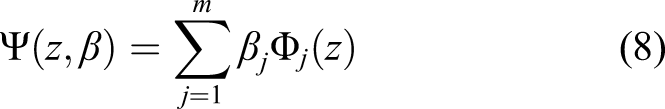$y_{d} = {\hat{Ψ}}_{h} (z)$ its estimated kernel density. A linear regression model of Legendre orthogonal polynomials is then used to approximate y_d as follows

Ψ (z, β) = \sum_{j = 1}^{m} β_{j} Φ_{j} (z)

(8)where Φ_j(z) is the jth Legendre polynomial and β_j is the jth coefficient. Legendre polynomials can be calculated from the formula given by Rodrigues (Askey, 2005)

Φ_{m} (z) = \frac{1}{2^{m} m!} \frac{d^{m}}{d z^{m}} [{(z^{2} - 1)}^{m}], m = 0,1,2, \dots

(9)where the first two terms are given by

Φ_{0} (z) = 1, Φ_{1} (z) = z

(10)

The coefficients of Legendre polynomials are obtained using the least square method. Letting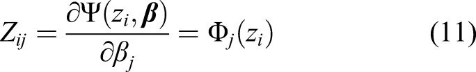

Z_{i j} = \frac{\partial Ψ (z_{i}, β)}{\partial β_{j}} = Φ_{j} (z_{i})

(11)the estimated coefficients are given by

\hat{β} = {(Z^{T} Z)}^{- 1} Z^{T} y_{d}

(12)

The coefficient $\hat{β}$ represents the kernel density–based features that can be used for classification using machine learning. The approximated density is then obtained using the following equation

Ψ_{a} = Z \hat{β}

(13)

The quality of the approximation was computed using root mean square error (RMSE) and Pearson’s correlation coefficient (PCC) as follows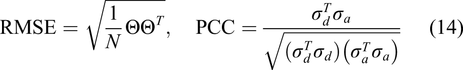

RMSE = \sqrt{\frac{1}{N} Θ Θ^{T}}, PCC = \frac{σ_{d}^{T} σ_{a}}{\sqrt{(σ_{d}^{T} σ_{d}) (σ_{a}^{T} σ_{a})}}

(14)where Θ = (y_d −Ψ_a) is the residual vector, N is the number of points in the density function,

σ_{d} = (y_{d} - E {y_{d}})

, and

σ_{a} = (Ψ_{a} - E {Ψ_{a}})

, where E{.} is the expected value.

3.2. Statistical feature extraction

The vibration data in the time waveform were used to extract statistical features. Eight statistical time-domain features including (1) mean, (2) root mean square, (3) SD, (4) peak value, (5) minimum value, (6) crest factor, (7) kurtosis value, and (8) skewness value were calculated.

3.3. SVM

The SVM is a supervised learning algorithm that can be used for classification and regression. SVM does indeed have a well-established theoretical background and intuitive geometrical interpretation. It is commonly used in the field of bearing diagnostics (Wu et al., 2012; Yang et al., 2007a; Zhang et al., 2013). SVM uses training data to define a hyperplane that maximizes the distance in the feature space between different classes (Bishop, 2006). The nearest data points to the hyperplane are called support vectors. To determine the optimal hyperplane, the following optimization problem is solved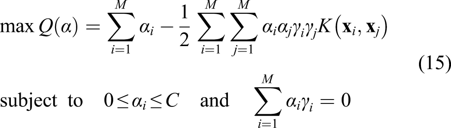

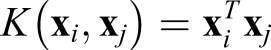
\begin{array}{l} max Q (α) = \sum_{i = 1}^{M} α_{i} - \frac{1}{2} \sum_{i = 1}^{M} \sum_{j = 1}^{M} α_{i} α_{j} γ_{i} γ_{j} K (x_{i}, x_{j}) \\ subject to 0 \leq α_{i} \leq C and \sum_{i = 1}^{M} α_{i} γ_{i} = 0 \end{array}

(15)where α_i denotes the Lagrangian multiplier. The training feature set and the desired output set are represented by x and γ, respectively. M is the number of training data samples, and K (x_i, x_j) is the kernel function that transforms the input features to a higher dimension space. For example, a linear kernel function can be expressed as

K (x_{i}, x_{j}) = x_{i}^{T} x_{j}

Finally, C denotes the box constraint, which controls the values of the Lagrangian multiplier. A higher value of C corresponds to a higher misclassification cost, resulting in strict separation.

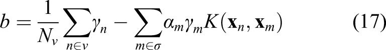
After the optimization problem is solved and the optimal αi parameters are obtained, a new test example can be identified using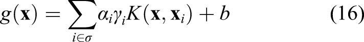

g (x) = \sum_{i \in σ} α_{i} γ_{i} K (x, x_{i}) + b

(16)where σ is the set of indices of the support vectors. Note that only the support vectors contribute to the prediction of new data. This is because αi is zero for data points that are not corresponding to the support vectors. The bias b in equation (16) can be obtained as follows

b = \frac{1}{N_{ν}} \sum_{n \in ν} γ_{n} - \sum_{m \in σ} α_{m} γ_{m} K (x_{n}, x_{m})

(17)where ν is the set of indices of the points that have 0 ≤ α_n ≤ C.

SVM was originally developed for binary classification (Cortes and Vapnik, 1995). The applicability of SVM was then applied to multi-class classification problems with a series of binary classifications (Schölkopf et al., 1999; Vapnik, 1998) using various approaches such as one-versus-all and one-versus-one (OVO). The OVO approach was used in this study because of its ability to train fast (Wang and Xue, 2014).

4. Results and discussion

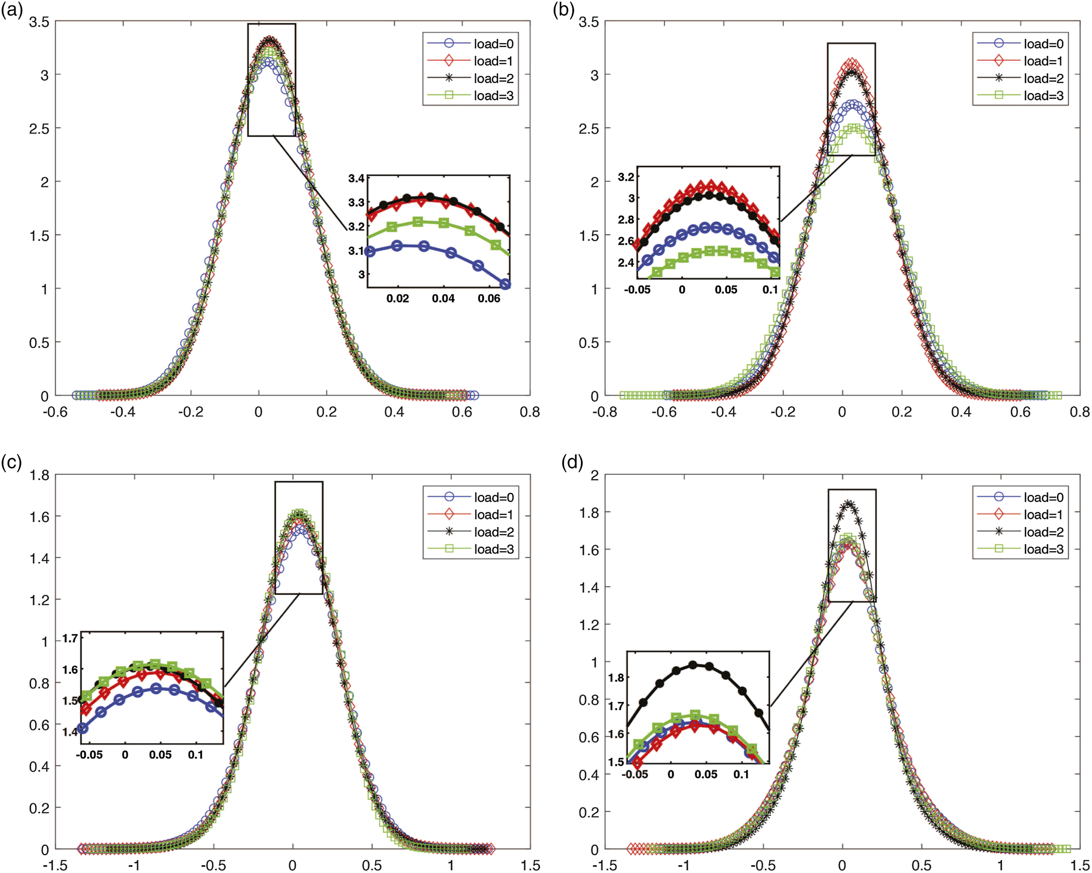
Samples of the estimated density distributions for the acceleration data of the DE and FE bearings at various motor loads and their corresponding speeds are shown in Figures 5 and 6, respectively. Various bearing conditions were investigated, and the results can be summarized as follows.

Figure 5.

Density distributions for various DE bearing classes with a DE-positioned sensor. (a) Healthy bearings. (b) Bearings with ball defect (0.007 in.). (c) Bearings with inner race defect (0.007 in.). (d) Bearings with outer race defect (0.007 in.). DE: drive end.

Figure 6.

Density distributions for various drive end bearing classes with a fan end–positioned sensor. (a) Healthy bearings. (b) Bearings with ball defect (0.007 in.). (c) Bearings with inner race defect (0.007 in.). (d) Bearings with outer race defect (0.007 in.).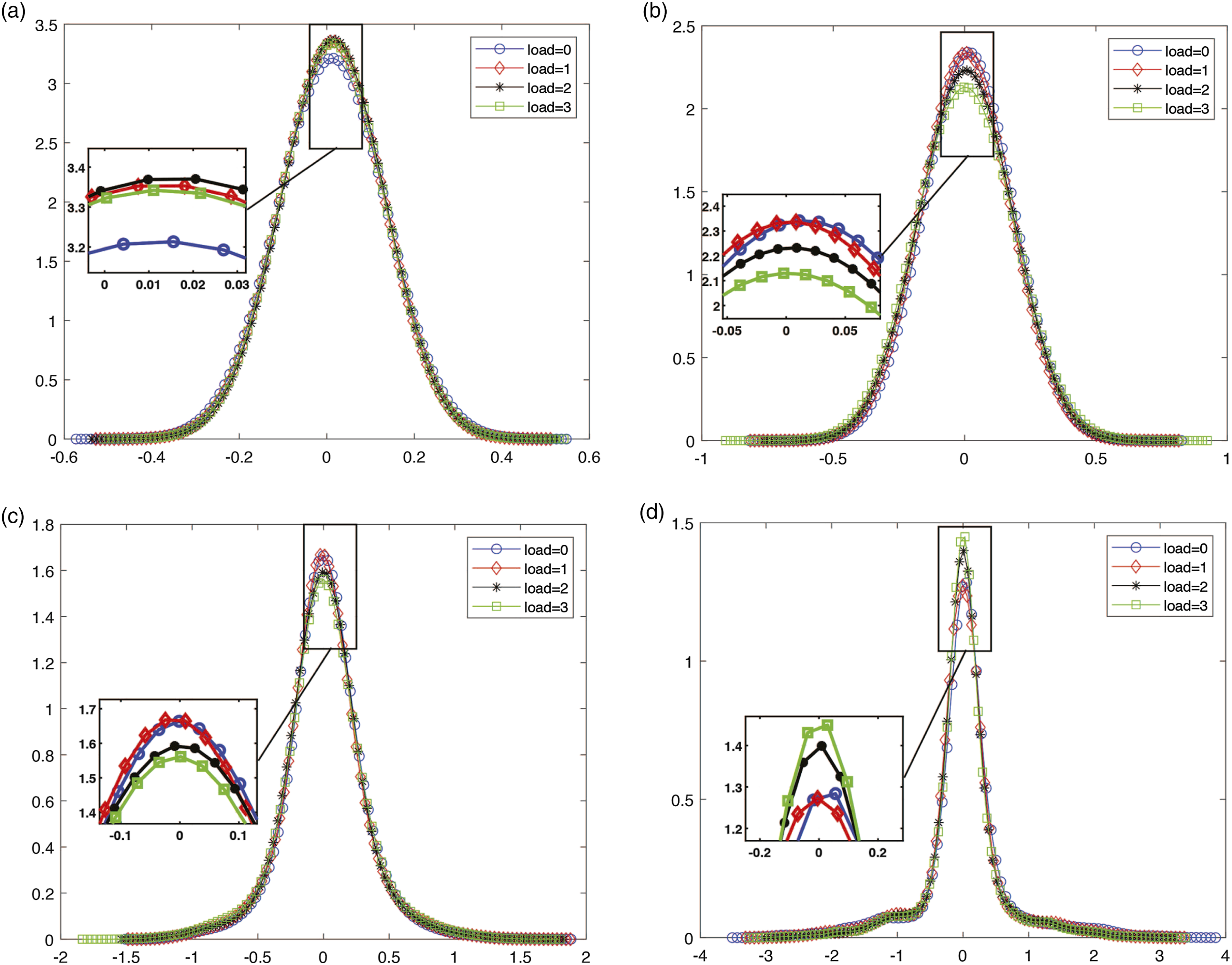

4.1. Effect of bearing condition

It can be observed that all the estimated density profiles have a symmetric unimodal distribution, which indicates that the states of the system are more frequent around one mode of the system. All distributions have a single peak approximately around zero for the different bearing conditions. However, the healthy condition has a higher density amplitude than other bearing conditions. This stems from the fact that the healthy bearing states are denser around zero. The inner and outer race bearing conditions seem to have lower density amplitudes. Density distributions also show that the outer race condition has the highest SD (wider density distribution) compared with other conditions because the vibration range reaches the highest in the outer race bearing condition (up to 3). Conversely, the healthy bearing condition seems to have the lowest vibration amplitude range.

4.2. Effect of sensor location

Different information can be extracted from a comparison of the density distributions of the vibration signals of the DE-positioned sensor and the FE-positioned sensor. For example, the DE sensor location provides more information in a comparison between the healthy bearing condition and the defective ball condition, although they look almost the same if we use the FE signal distribution. The DE-positioned sensor also provides more information in distinguishing between bearings with outer race and inner race conditions. On the other hand, the FE signal distribution is more capable of distinguishing the inner race condition from the healthy and ball conditions by having the lowest density amplitude.

4.3. Effect of the operating conditions

The relationship between the density distribution and the motor load and the rotational speed is nonlinear. For some conditions, such as for the bearing with the OR defect, increasing the motor load and therefore decreasing the rotational speed causes an increase in the density amplitude. However, this is not the case for B and IR defect conditions.

The PST method was applied by mapping the data onto a density space for each condition and then approximating these densities using Legendre polynomials. After the density plots were estimated, the plots were then expanded in a series of Legendre polynomials of order 30. The order of Legendre polynomials was selected based on the best fit between the actual and the approximate densities by calculating the RMSE and PCC.

To illustrate the extracted PST features, Figure 7 presents the first five features of the DE sensor (indexed from 1 to 5) and the first five features of the FE sensor (indexed from 6 to 10). The shown features are for various bearing conditions (0.007 in. of fault diameter) under zero motor load. It can be seen from the figure that the PST features reveal informative patterns about the intrinsic dynamics of the system and distinguish between different bearing conditions. For example, the first five features (indexed from 1 to 5) that correspond to the DE sensor data separate distinctly between the bearing conditions with approximately equal distances. On the other hand, features 6, 8, and 10 separate healthy and ball bearings from inner and outer race conditions. Features 7 and 9 separate inner race condition from other bearing condition as demonstrated previously by the FE density distribution. These results show the rich information extracted from the PST to distinguish between different bearing conditions. It also shows the importance of using the information from both the DE and FE sensors where the information provided from the extracted features are evident. This distinction was not clear when the density distributions were analyzed, which again proves the predictive strength of the extracted features.

Figure 7.

A comparison between the extracted phase space topology features and bearing conditions.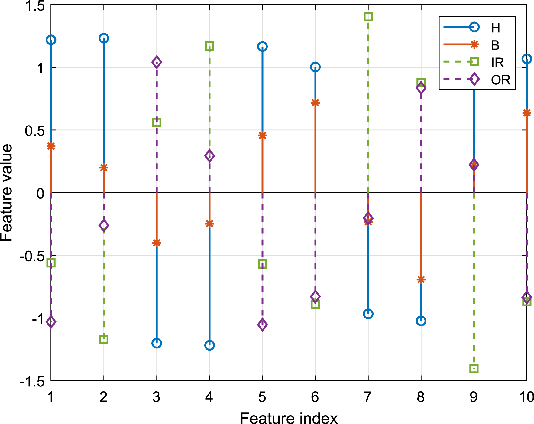

Similarly, the statistical time-domain features extracted for the signals of DE- and FE-positioned sensors are shown in Figure 8. The shown features are for various bearing conditions (0.007 in. of fault diameter) under zero motor load. Note that the feature index 1–8 in Figure 8 corresponds to the feature numbers defined in Section 3.2. It can be seen from Figure 8(a) that most of the features separate the outer race condition from the other conditions. The main challenge these features face is distinguishing between healthy and ball conditions. On the other hand, in Figure 8(b), feature 1 separates between healthy and defective conditions. Feature 6 separates B defect from other conditions. It should be emphasized that the above observations are at a single operating condition and for one fault diameter, that is 0.007 in. Our goal is to develop an algorithm to distinguish between different faults at various operating conditions; thus, all the above features will be used.

Figure 8.

A comparison between the extracted statistical time-domain features and bearing conditions. (a) The signal of drive end–positioned sensor. (b) The signal of fan end–positioned sensor.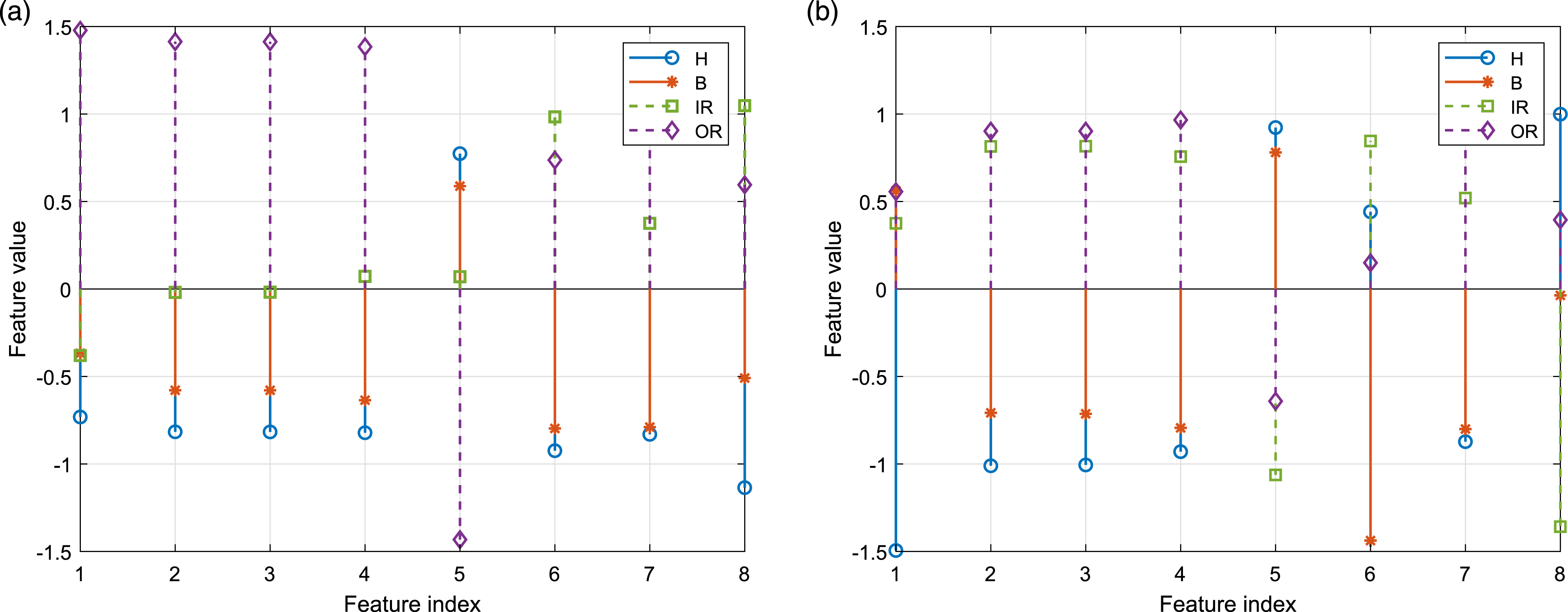

4.4. Fault identification

In the previous section, we illustrated how the features are extracted using PST and statistical time-domain measures. Next, the extracted features are used to classify and predict various bearing conditions (H, B, IR, and OR). For each set of data, 36 features (10 PST features and 8 statistical features for each acceleration signal) were standardized and then used as inputs to train a linear SVM classifier. An SVM classifier was trained using 60% of the data samples (300 cases) and a five-fold cross-validation algorithm. For testing the classifier, 40% of the data samples (200 cases) were used. The box constraint parameter was optimized by minimizing the k-fold cross-validation loss to find the optimal linear SVM. Figure 9 shows the estimated objective function for different values of the box constraint parameter. It can be seen that the optimal value of the box constraint was around 0.33.

Figure 9.

Optimal box constraint parameter.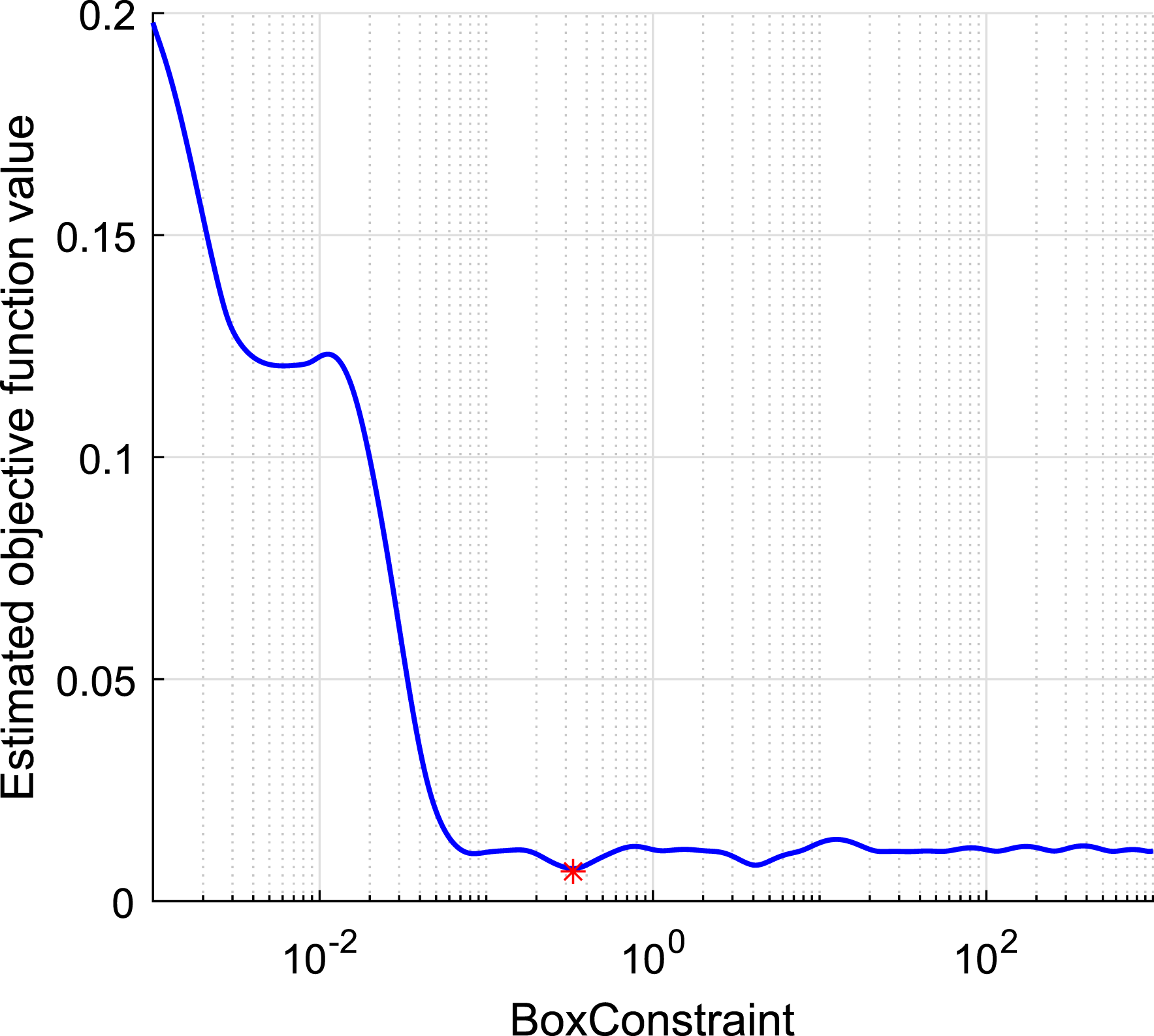

The effectiveness of the classification models is illustrated using the confusion matrix plots. The training and test confusion matrices of the linear SVM are shown in Tables 3 and 4, respectively. The diagonal cells in the confusion matrix show the number and percentage of correct classifications, whereas the misclassified predictions are the off-diagonal cells. For example, in Table 4, the linear SVM correctly predicted 56 cases as a healthy bearing condition, 48 cases as a defective ball condition, 46 cases as a defective inner race condition, and 48 cases as a defective outer race condition. Of 200 total test samples, 2 inner race cases were misclassified as ball cases.

Table 3.

Prediction of various defect classes for training data.

		Target class				Recall (%)	Precision (%)
		H	B	IR	OR	Recall (%)	Precision (%)
Output class	H	84	0	0	0	100.0	100.0
	H	28.0%	0.0%	0.0%	0.0%	100.0	100.0
	B	0	72	0	0	100.0	100.0
	B	0.0%	24.0%	0.0%	0.0%	100.0	100.0
	IR	0	0	72	0	100.0	100.0
	IR	0.0%	0.0%	24.0%	0.0%	100.0	100.0
	OR	0	0	0	72	100.0	100.0
	OR	0.0%	0.0%	0.0%	24.0%	100.0	100.0
						Accuracy 100.0%

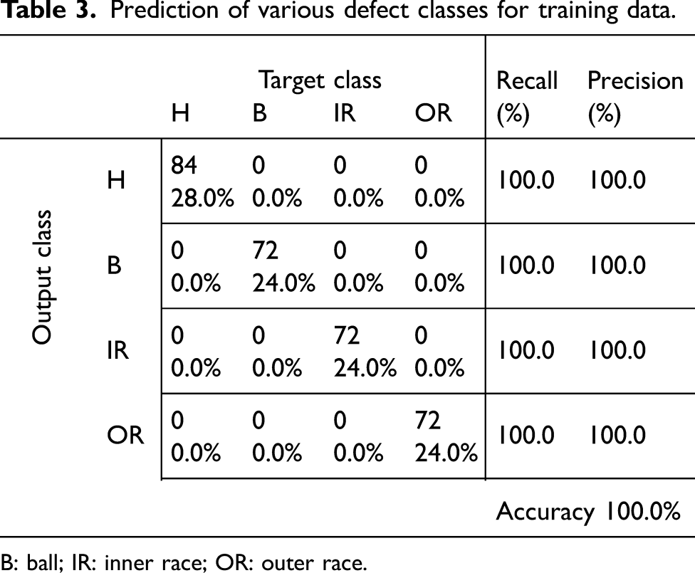
B: ball; IR: inner race; OR: outer race.

Table 4.

Prediction of various defect classes for test data.

		Target class				Recall (%)	Precision (%)
		H	B	IR	OR	Recall (%)	Precision (%)
Output class	H	56	0	0	0	100.0	100.0
	H	28.0%	0.0%	0.0%	0.0%	100.0	100.0
	B	0	48	2	0	100.0	96.0
	B	0.0%	24.0%	1.0%	0.0%	100.0	96.0
	IR	0	0	46	0	95.8	100.0
	IR	0.0%	0.0%	23.0%	0.0%	95.8	100.0
	OR	0	0	0	48	100.0	100.0
	OR	0.0%	0.0%	0.0%	24.0%	100.0	100.0
						Accuracy 99.0%

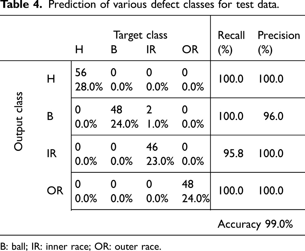
B: ball; IR: inner race; OR: outer race.

Various metrics can be calculated from the confusion matrix such as precision, recall, and overall accuracy (Mohamad et al., 2018b) to define the performance of the classifier. Precision measures the rate of correct predictions from all predictions for each class and indicates how often the classifier’s prediction is correct. For a given class, recall measures the correctly predicted rate of the actual samples. Ideally, the goal is to achieve a classifier with high recall and high precision. Finally, the classifier’s overall accuracy is the correct prediction rate.

The results of the training and test confusion matrices (Tables 3 and 4) indicate the following.

The classifier model was able to identify a hyperplane in the feature space that can separate all training set samples with 100% overall accuracy, as shown in Table 3.

The classification of the test data indicates an overall accuracy of 99% for predicting different bearing conditions under various motor load/speed conditions.

The classifier was able to detect anomalous behavior in the system by distinguishing healthy bearings from defective bearings. This has far-reaching practical advantages in system condition monitoring applications.

The classifier was able to predict all the test cases with over 95% accuracy, recall, and precision for each bearing condition.

The PST-extracted features provide valuable information in characterizing the dynamics of various bearing conditions, regardless of the fault level and severity.

Notably, no a priori knowledge of the system was included in the extracted features. This implies that the PST approach can be conveniently applied to diverse dynamical systems in an automated process with a minimal need for adaptation or reliance on expert knowledge about the system.

4.5. Comparison with envelope analysis

One of the main techniques used currently in bearing diagnostics is the envelope analysis technique, which is based on the demodulation of high-frequency resonance associated with bearing element impacts. Envelope spectrum helps in showing the bearing defect frequencies, which are produced by the repeated impacts each time the rolling element strikes a defect. The bearing defect frequencies can be calculated as follows. Ball pass frequency, outer race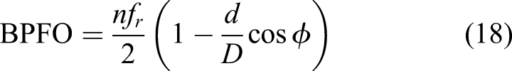

BPFO = \frac{n f_{r}}{2} (1 - \frac{d}{D} \cos ϕ)

(18)

Ball pass frequency, inner race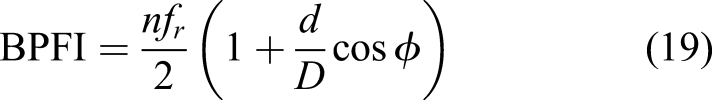

BPFI = \frac{n f_{r}}{2} (1 + \frac{d}{D} \cos ϕ)

(19)

Fundamental train frequency (cage speed)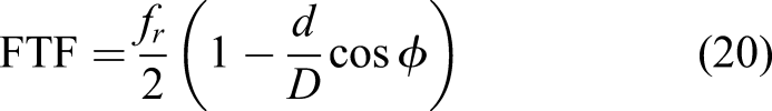

FTF = \frac{f_{r}}{2} (1 - \frac{d}{D} \cos ϕ)

(20)

Ball spin frequency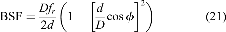

BSF = \frac{D f_{r}}{2 d} (1 - {[\frac{d}{D} \cos ϕ]}^{2})

(21)where f_r is the rotational speed of the shaft, n is the number of rolling elements, ϕ is the angle of the load from the radial plane, d is the rolling element diameter, and D is the bearing pitch diameter. In reality, the defect frequencies can differ from the calculated frequencies. This is owing to the fact that these frequencies are derived based on the assumption of no slip, which is not accurate. The calculated defect frequencies per shaft speed for DE bearing are BPFO = 3.58, BPFI = 5.42, FTF = 0.40, and BSF = 4.71, respectively.

The signal is band-pass filtered around a frequency that has the maximum signal-to-noise ratio to find the envelope spectrum, and then the Hilbert transform is used to find the envelope. Finally, the envelope spectrum is determined by the FFT.

The successful implementation of envelope analysis requires a suitable selection of central frequency and range for the band-pass filter. In this work, we used the kurtogram to select these parameters. The kurtogram is a representation of spectral kurtosis (SK) in the frequency and frequency resolution plane. The optimal combination of frequency and window length which maximize SK is chosen. In this work, the fast computation algorithm in Antoni (2007) was used.

Figure 10 shows the envelope analysis procedure for bearings with IR defects. The raw vibration data for the inner race bearing condition are first presented in Figure 10(a). The kurtogram for different frequencies and frequency resolutions is shown in Figure 10(b). It can be seen that the maximum SK (SK_max = 2.6) occurs at a central frequency of 3000 Hz and a bandwidth of 6000 HZ. The envelope of the filtered signal using the optimal parameter is constructed in Figure 10(c). Finally, the envelope spectrum is determined and presented in Figure 10(d), which shows the first harmonic in addition to the inner race ball pass frequency.

Figure 10.

Envelope analysis for inner race bearing condition. (a) Raw vibration signal. (b) Kurtogram. (c) Envelope of filtered signal. (d) Envelope spectrum.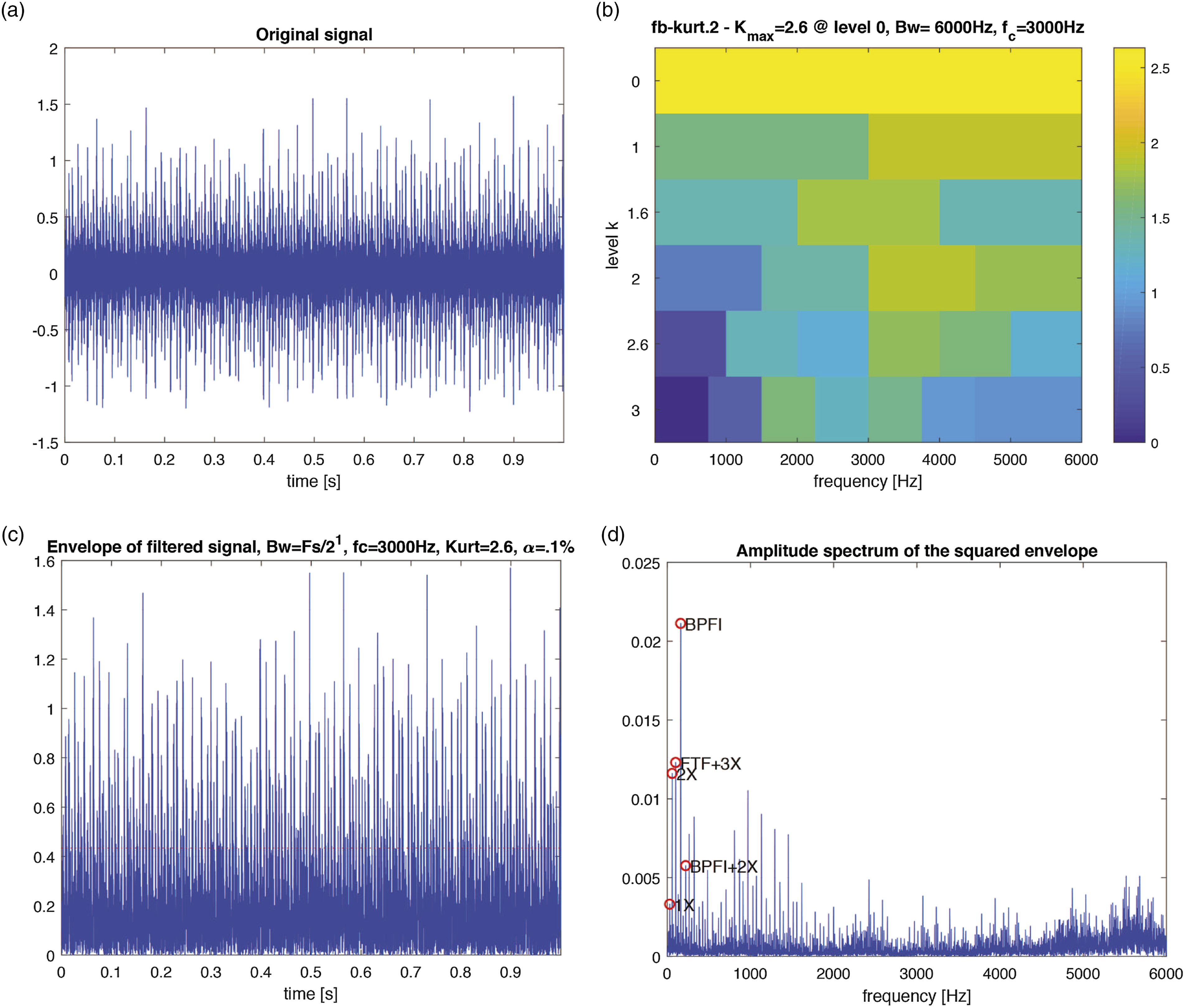

Similarly, Figure 11 shows the envelope spectrum for OR and B defects. The ball pass outer race frequency is clearly shown in Figure 11(a), and the ball spin frequency for the B defect condition is presented in Figure 11(b). Note, however, that this frequency is not always visible, for instance, see Figure 11(a). This is indeed a disadvantage of the envelope spectrum method.

Figure 11.

Envelope spectrum. (a) Outer race bearing condition. (b) Ball bearing condition.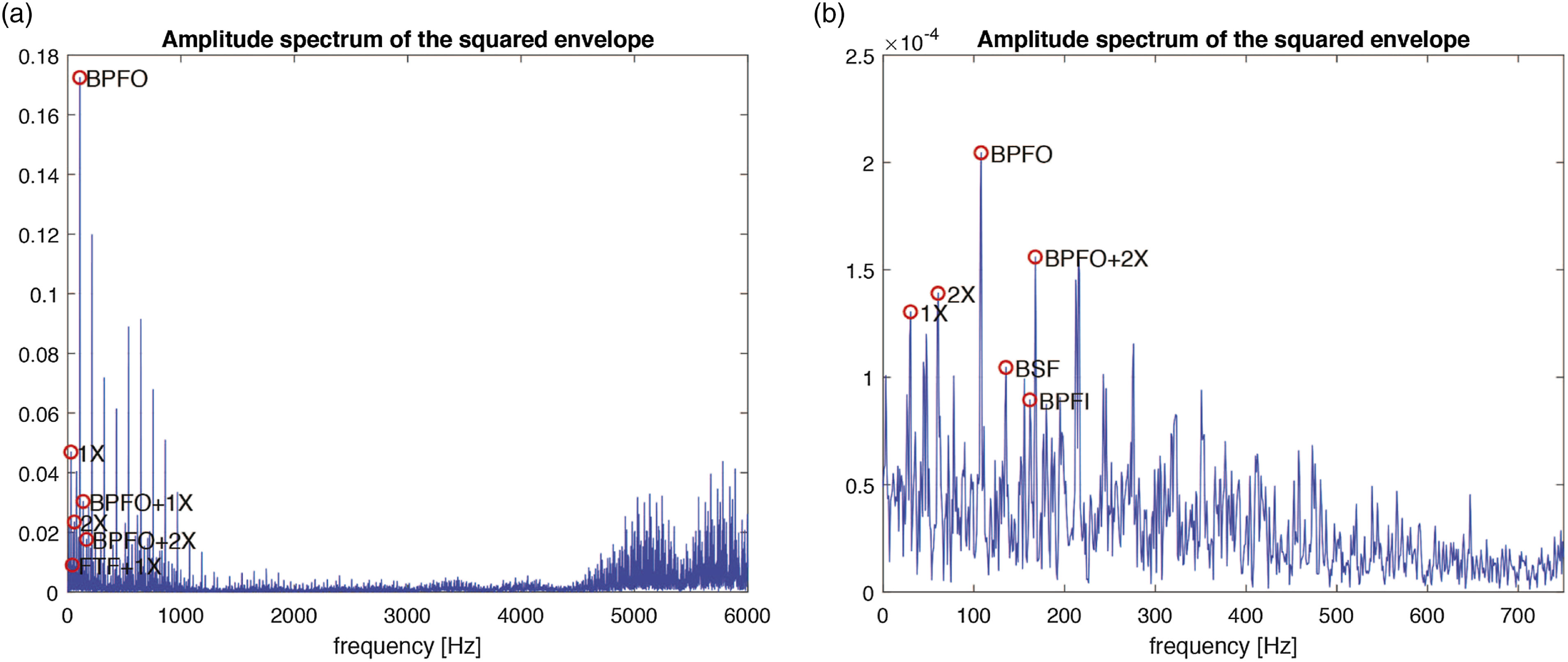

To classify the bearing conditions, features were extracted from the envelope spectrum of the DE and FE signals. At each peak, the location f_p and the amplitude A_p of the peak were considered as features. In addition, the energy of the peak E_p can be calculated as follows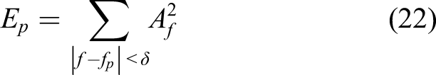

E_{p} = \sum_{| f - f_{p} | < δ} A_{f}^{2}

(22)where δ is the width of the peak.

The extracted features were used as inputs to train an SVM classifier. Various SVMs were trained using 60% of the data samples (300 cases) and a cross-validation algorithm with five folds. 40% of the data samples (200 cases) were used for testing the classifier. The box constraint parameter was optimized by minimizing the k-fold cross-validation loss to find the optimal SVM.

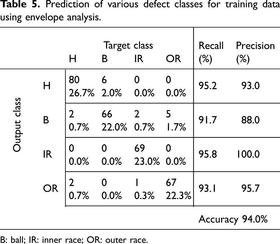
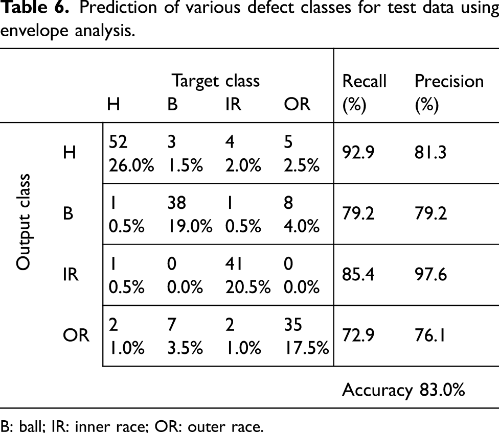
The training and test confusion matrices of the SVM are shown in Tables 5 and 6, respectively. The results indicate the following.

The SVM classifier was able to determine a hyperplane in the training feature space that can separate training samples with a high overall accuracy of 94.0%, as presented in Table 5.

The classification of the test data, presented by the confusion matrix in Table 6, indicates an overall accuracy of 83% for predicting different bearing conditions.

Anomaly detection between healthy and defective bearing conditions was achieved with 81.3% precision and 92.9% recall.

Bearings with OR defects had the lowest metric performance, followed by the B defect.

Table 5.

Prediction of various defect classes for training data using envelope analysis.

		Target class				Recall (%)	Precision (%)
		H	B	IR	OR	Recall (%)	Precision (%)
Output class	H	80	6	0	0	95.2	93.0
	H	26.7%	2.0%	0.0%	0.0%	95.2	93.0
	B	2	66	2	5	91.7	88.0
	B	0.7%	22.0%	0.7%	1.7%	91.7	88.0
	IR	0	0	69	0	95.8	100.0
	IR	0.0%	0.0%	23.0%	0.0%	95.8	100.0
	OR	2	0	1	67	93.1	95.7
	OR	0.7%	0.0%	0.3%	22.3%	93.1	95.7
						Accuracy 94.0%

B: ball; IR: inner race; OR: outer race.

Table 6.

Prediction of various defect classes for test data using envelope analysis.

		Target class				Recall (%)	Precision (%)
		H	B	IR	OR	Recall (%)	Precision (%)
Output class	H	52	3	4	5	92.9	81.3
	H	26.0%	1.5%	2.0%	2.5%	92.9	81.3
	B	1	38	1	8	79.2	79.2
	B	0.5%	19.0%	0.5%	4.0%	79.2	79.2
	IR	1	0	41	0	85.4	97.6
	IR	0.5%	0.0%	20.5%	0.0%	85.4	97.6
	OR	2	7	2	35	72.9	76.1
	OR	1.0%	3.5%	1.0%	17.5%	72.9	76.1
						Accuracy 83.0%

B: ball; IR: inner race; OR: outer race.

In conclusion, a comparison with Tables 3 and 4 demonstrates that the PST method performed consistently better than the envelope analysis method and, in fact, does so without an a priori specification of defect frequencies.

5. Fault severity classification

The second phase of the study investigated the estimation of the severity of the faults using the extracted features. If a fault was identified, the severity of the predicted fault, or the amount of degradation, was determined by building an additional linear SVM for each fault. The extracted features, including the PST features and the time-domain statistical features, were used as inputs to an SVM to predict the diameter of the fault (0.007, 0.014, or 0.021). Three SVMs were trained and optimized for each defective bearing condition using 60% of the data set. The other 40% of the data set was used for testing. Classification results are presented by means of confusion matrices in Tables 7–9 and summarized as follows.

The classifier was able to predict the diameter of the fault for inner race and outer race bearing conditions with 100% overall accuracy, 100% recall, and 100% precision.

The extracted features provided accurate information to predict the level of degradation of bearing with inner race and OR defects.

Predicting the level of degradation for B defects was achieved with a virtually perfect overall accuracy for the smaller diameter faults (0.007 in.) and an overall accuracy of 90.0% for the larger diameter faults.

The classifier was able to predict the B defect with 0.007 in. fault diameter with 100% recall and 100% precision. However, the classifier incorrectly predicted 3 cases of B defects with 0.014 in. of fault diameter.

Table 7.

Prediction of various fault diameters for test data of defective ball bearing condition.

		Target class			Recall (%)	Precision (%)
		0.007	0.014	0.021	Recall (%)	Precision (%)
Output class	0.007	16	0	0	100.0	100.0
	0.007	33.3%	0.0%	0.0%	100.0	100.0
	0.014	0	9	0	75.0	100.0
	0.014	0.0%	18.8%	0.0%	75.0	100.0
	0.021	0	3	20	100.0	87.0
	0.021	0.0%	6.3%	41.7%	100.0	87.0
					Accuracy 93.8%

Table 8.

Prediction of various fault diameters for test data of defective inner race bearing condition.

		Target class			Recall (%)	Precision (%)
		0.007	0.014	0.021	Recall (%)	Precision (%)
Output class	0.007	13	0	0	100.0	100.0
	0.007	27.1%	0.0%	0.0%	100.0	100.0
	0.014	0	17	0	100.0	100.0
	0.014	0.0%	35.4%	0.0%	100.0	100.0
	0.021	0	0	18	100.0	100.0
	0.021	0.0%	0.0%	37.5%	100.0	100.0
					Accuracy 100.0%

Table 9.

Prediction of various fault diameters for test data of defective outer race bearing condition.

		Target class			Recall (%)	Precision (%)
		0.007	0.014	0.021	Recall (%)	Precision (%)
Output class	0.007	17	0	0	100.0	100.0
	0.007	35.4%	0.0%	0.0%	100.0	100.0
	0.014	0	15	0	100.0	100.0
	0.014	0.0%	31.3%	0.0%	100.0	100.0
	0.021	0	0	16	100.0	100.0
	0.021	0.0%	0.0%	33.3%	100.0	100.0
					Accuracy 100.0%

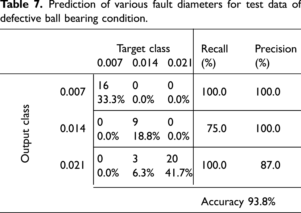
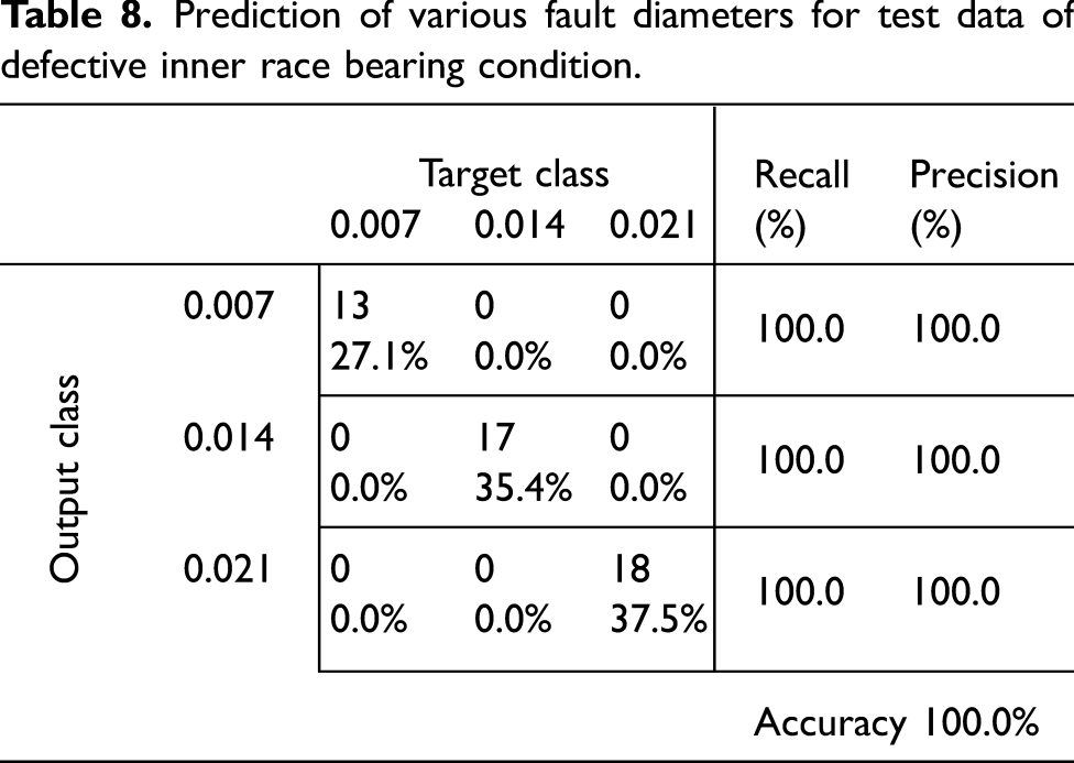
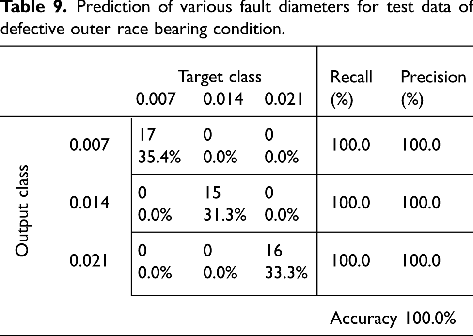
From the above results, it is evident that the PST method effectively determines the severity level of various bearing defects.

6. Conclusion

The PST family of methods is built on studying the basic nonlinear physics of the system which could have valuable insights. Bearings under various operating conditions including motor load and speed were investigated. The study demonstrates that the PST method, combined with statistical measures, provides rich information about the status of the health of the bearing. Moreover, the results show that the innovative PST procedure has exceptional performance in detecting and identifying faults.

The PST has significant advantages in identifying the level of degradation of the bearing faults for inner race and outer race bearing conditions. For ball bearing defects, the PST achieved a perfect prediction accuracy in identifying the smaller diameter faults (i.e. fault diameter of 0.007 in.) and acceptable accuracy in identifying the larger diameter faults (i.e. fault diameter of 0.014 and 0.021 in.). To improve the accuracy, we plan to explore selecting an optimal feature set for the ball condition using mutual information as a feature ranking technique.

A comparison with the envelope analysis method was performed and discussed in detail. Results show that the PST method performed consistently better than the envelope analysis method. Future work should investigate bearing diagnostics under a variable speed domain, and the PST family of methods should be adapted and validated for transfer learning applications.

Footnotes

Acknowledgements

We thank ONR’s support and are honored by their recognition of the importance of this research, and acknowledge continued support from Capt. Lynn Petersen.

Declaration of conflicting interests

The authors declared no potential conflicts of interest with respect to the research, authorship, and/or publication of this article.

Funding

The authors disclosed receipt of the following financial support for the research, authorship, and/or publication of this article: US Office of Naval Research (Grants No. ONR N0014-15-1-2311 and ONR N00014-19-1-2070).

ORCID iD

T Haj Mohamad

References

Ali

Fnaiech

Saidi

, et al. (2015) Application of empirical mode decomposition and artificial neural network for automatic bearing fault diagnosis based on vibration signals. Applied Acoustics 89: 16–27.

Antoni

(2007) Fast computation of the kurtogram for the detection of transient faults. Mechanical Systems and Signal Processing 21(1): 108–124.

Askey

(2005) The 1839 paper on permutations: its relation to the rodrigues formula and further developments. Mathematics and Social Utopias in France: Olinde Rodrigues and His Times 28: 105–118.

Bishop

(2006) Pattern Recognition and Machine Learning. New York: Springer-Verlag.

Borghesani

Pennacchi

Randall

, et al. (2013) Application of cepstrum pre-whitening for the diagnosis of bearing faults under variable speed conditions. Mechanical Systems and Signal Processing 36(2): 370–384.

Cocconcelli

Zimroz

Rubini

, et al. (2012) STFT based approach for ball bearing fault detection in a varying speed motor. In: Condition Monitoring of Machinery in Non-Stationary Operations. Berlin, Heidelberg: Springer, 41–50.

Cortes

Vapnik

(1995) Machine learning. Machine Learning 20: 273–297.

Liu

Huang

, et al. (2017) An optimal ensemble empirical mode decomposition method for vibration signal decomposition. Journal of Vibration and Acoustics 139(3): 031003.

Gan

Wang

Zhu

(2016) Construction of hierarchical diagnosis network based on deep learning and its application in the fault pattern recognition of rolling element bearings. Mechanical Systems and Signal Processing 72–73: 92–104.

10.

Gao

Liang

Chen

, et al. (2015) Feature extraction and recognition for rolling element bearing fault utilizing short-time fourier transform and non-negative matrix factorization. Chinese Journal of Mechanical Engineering 28(1): 96–105.

11.

George

Mishra

Dwivedi

(2018) Mahalanobis distance among the phase portraits as damage feature. Structural Health Monitoring 17(4): 869–887.

12.

Gryllias

Antoniadis

(2012) A support vector machine approach based on physical model training for rolling element bearing fault detection in industrial environments. Engineering Applications of Artificial Intelligence 25(2): 326–344. Special section: local search algorithms for real-world scheduling and planning.

13.

Randall

(2000) Optimisation of bearing diagnostic techniques using simulated and actual bearing fault signals. Mechanical Systems and Signal Processing 14(5): 763–788.

14.

Honarvar

Martin

(1997) New statistical moments for diagnostics of rolling element bearings. Journal of Manufacturing Science and Engineering 119(3): 425–432.

15.

Jung

Koh

B-H

(2015) Wavelet energy-based visualization and classification of high-dimensional signal for bearing fault detection. Knowledge and Information Systems 44(1): 197–215.

16.

Kankar

Sharma

Harsha

(2011a) Rolling element bearing fault diagnosis using autocorrelation and continuous wavelet transform. Journal of Vibration and Control 17(14): 2081–2094.

17.

Kankar

Sharma

Harsha

(2011b) Rolling element bearing fault diagnosis using wavelet transform. Neurocomputing 74(10): 1638–1645.

18.

Kappaganthu

Nataraj

(2011a) Feature selection for fault detection in rolling element bearings using mutual information. Journal of Vibration and Acoustics 133(6).

19.

Kappaganthu

Nataraj

(2011b) Modeling and analysis of outer race defects in rolling element bearings. Advances in Vibration Engineering 11(4): 371–384.

20.

Konar

Chattopadhyay

(2011) Bearing fault detection of induction motor using wavelet and support vector machines (SVMS). Applied Soft Computing 11(6): 4203–4211.

21.

Kwuimy

Mohamad

Nataraj

(2018) Using the Gottwald and Melbournes 0-1 test and the Hugichi fractal dimension to detect chaos in defective and healthy ball bearings. MATEC Web of Conferences 241: 01017.

22.

Lei

Lin

, et al. (2013) A review on empirical mode decomposition in fault diagnosis of rotating machinery. Mechanical Systems and Signal Processing 35(1–2): 108–126.

23.

Loparo

(2003) Bearing vibration data set. Available at: http://www.eecs.cwru.edu/laboratory/bearing/download.htm.

24.

Maraini

Nataraj

(2018) Nonlinear analysis of a rotor-bearing system using describing functions. Journal of Sound and Vibration 420: 227–241.

25.

Ming

Chen

Dong

(2011) Weak fault feature extraction of rolling bearing based on cyclic wiener filter and envelope spectrum. Mechanical Systems and Signal Processing 25(5): 1773–1785.

26.

Mohamad

Cavalini

Steffen

, et al. (2018a) Detection of cracks in a rotating shaft using density characterization of orbit plots. In: International conference on rotor dynamics, Rio de Janeiro, Brazil, 23–27 September, pp. 90–104. Cham, Switzerland: Springer.

27.

Mohamad

Chen

Chaudhry

, et al. (2018b) Gear fault detection using recurrence quantification analysis and support vector machine. Journal of Software Engineering and Applications 11(05): 181–203.

28.

Mohamad

Kwuimy

Nataraj

(2018c) Multi-speed multi-load bearing diagnostics using extended phase space topology. MATEC Web of Conferences 241: 01011.

29.

Mohamad

Nataraj

(2017) Gear fault diagnostics using extended phase space topology. In: Annual conference of the prognostics and health management society, 2–5 October 2017, Florida.

30.

Mohamad

Nazari

Nataraj

(2019) A review of phase space topology methods for vibration-based fault diagnostics in nonlinear systems. Journal of Vibration Engineering & Technologies 8: 393–401.

31.

Mohamad

Samadani

Nataraj

(2018d) Rolling element bearing diagnostics using extended phase space topology. Journal of Vibration and Acoustics 140(6): 061009.

32.

Nichols

(2003) Structural health monitoring of offshore structures using ambient excitation. Applied Ocean Research 25(3): 101–114.

33.

Nie

Hao

(2012) Using vibration phase space topology changes for structural damage detection. Structural Health Monitoring: An International Journal 11(5): 538–557.

34.

Nikolaou

Antoniadis

(2002) Rolling element bearing fault diagnosis using wavelet packets. NDT & E International 35(3): 197–205.

35.

Nolte

(2010) The tangled tale of phase space. Physics Today 63(4): 33–38.

36.

Pandya

Upadhyay

Harsha

(2013) Fault diagnosis of rolling element bearing with intrinsic mode function of acoustic emission data using APF-KNN. Expert Systems with Applications 40(10): 4137–4145.

37.

Patel

Tandon

Pandey

(2012) Defect detection in deep groove ball bearing in presence of external vibration using envelope analysis and duffing oscillator. Measurement 45(5): 960–970.

38.

Patil

Gaikwad

Kulkarni

(2016) Bearing fault diagnosis using discrete wavelet transform and artificial neural network. In: 2016 2nd international conference on applied and theoretical computing and communication technology (iCATccT), Bangalore, India, 21–23 July 2016, pp. 399–405. Piscataway, NJ: IEEE.

39.

Peng

Chu

(2004) Application of the wavelet transform in machine condition monitoring and fault diagnostics: a review with bibliography. Mechanical Systems and Signal Processing 18(2): 199–221.

40.

Peng

Tse

Chu

(2005) A comparison study of improved Hilbert–Huang transform and wavelet transform: application to fault diagnosis for rolling bearing. Mechanical Systems and Signal Processing 19(5): 974–988.

41.

Peter

Peng

Yam

(2001) Wavelet analysis and envelope detection for rolling element bearing fault diagnosis their effectiveness and flexibilities. Journal of Vibration and Acoustics 123(3): 303–310.

42.

Prabhakar

Mohanty

Sekhar

(2002) Application of discrete wavelet transform for detection of ball bearing race faults. Tribology International 35(12): 793–800.

43.

Prieto

Cirrincione

Espinosa

, et al. (2013) Bearing fault detection by a novel condition-monitoring scheme based on statistical-time features and neural networks. IEEE Transactions on Industrial Electronics 60(8): 3398–3407.

44.

Rai

Mohanty

(2007) Bearing fault diagnosis using FFT of intrinsic mode functions in Hilbert–Huang transform. Mechanical Systems and Signal Processing 21(6): 2607–2615.

45.

Randall

(2011) Vibration-Based Condition Monitoring: Industrial, Aerospace and Automotive Applications. West Sussex, UK: John Wiley & Sons.

46.

Randall

Antoni

(2011) Rolling element bearing diagnostics-A tutorial. Mechanical Systems and Signal Processing 25(2): 485–520.

47.

Rubini

Meneghetti

(2001) Application of the envelope and wavelet transform analyses for the diagnosis of incipient faults in ball bearings. Mechanical Systems and Signal Processing 15(2): 287–302.

48.

Samadani

Kwuimy

Nataraj

(2013) Diagnostics of a nonlinear pendulum using computational intelligence. In: ASME 2013 dynamic systems and control conference, Palo Alto, CA, 21–23 October 2013. New York: American Society of Mechanical Engineers (ASME).

49.

Samadani

Mohamad

Nataraj

(2016) Feature extraction for bearing diagnostics based on the characterization of orbit plots with orthogonal functions. In: ASME 2016 international design engineering technical conferences and computers and information in engineering conference, Charlotte, NC, 21–24 August 2016, pp. V008T10A026. New York: American Society of Mechanical Engineers (ASME).

50.

Samanta

Al-Balushi

(2003) Artificial neural network based fault diagnostics of rolling element bearings using time-domain features. Mechanical Systems and Signal Processing 17(2): 317–328.

51.

Schölkopf

Burges

Smola

(1999) Advances in Kernel Methods: Support Vector Learning. Cambridge, MA: MIT Press.

52.

Seryasat

Honarvar

Rahmani

, et al. (2010) Multi-fault diagnosis of ball bearing using FFT, wavelet energy entropy mean and root mean square (RMS). In: 2010 IEEE international conference on systems, man and cybernetics, Istanbul, Turkey, 10–13 October 2010, pp. 4295–4299. Piscataway, NJ: IEEE.

53.

Shibata

Takahashi

Shirai

(2000) Fault diagnosis of rotating machinery through visualisation of sound signals. Mechanical Systems and Signal Processing 14(2): 229–241.

54.

Silverman

(2018) Density Estimation for Statistics and Data Analysis. Boca Raton, FA: Chapman and Hall/CRC.

55.

Smith

Randall

(2015) Rolling element bearing diagnostics using the case western reserve university data: a benchmark study. Mechanical Systems and Signal Processing 64–65: 100–131.

56.

Sreejith

Verma

Srividya

(2008) Fault diagnosis of rolling element bearing using time-domain features and neural networks. In: 2008 IEEE region 10 and the third international conference on industrial and information systems, Kharagpur, India, 8–10 December 2008, pp. 1–6. Piscataway, NJ: IEEE.

57.

Todd

Nichols

Pecora

, et al. (2001) Vibration-based damage assessment utilizing state space geometry changes: local attractor variance ratio. Smart Materials and Structures 10(5): 1000–1008.

58.

Torkamani

Butcher

Todd

, et al. (2012) Hyperchaotic probe for damage identification using nonlinear prediction error. Mechanical Systems and Signal Processing 29: 457–473.

59.

Vapnik

(1998) Statistical Learning Theory. New York: Wiley.

60.

Wang

Xue

(2014) Multi-class support vector machine. In: Support Vector Machines Applications. Cham, Switzerland: Springer, pp. 23–48.

61.

S-D

P-H

C-W

, et al. (2012) Bearing fault diagnosis based on multiscale permutation entropy and support vector machine. Entropy 14(8): 1343–1356.

62.

Xiang

Zhong

Gao

(2015) Rolling element bearing fault detection using PPCA and spectral kurtosis. Measurement 75: 180–191.

63.

Yang

Mathew

(2005) Fault diagnosis of rolling element bearings using basis pursuit. Mechanical Systems and Signal Processing 19(2): 341–356.

64.

Yang

Cheng

(2007a) A fault diagnosis approach for roller bearing based on IMF envelope spectrum and SVM. Measurement 40(9): 943–950.

65.

Yang

Zhang

Zhu

(2007b) Intelligent fault diagnosis of rolling element bearing based on SVMS and fractal dimension. Mechanical Systems and Signal Processing 21(5): 2012–2024.

66.

Zhang

Liang

Zhou

, et al. (2015) A novel bearing fault diagnosis model integrated permutation entropy, ensemble empirical mode decomposition and optimized svm. Measurement 69: 164–179.

67.

Zhang

Zhou

(2013) Multi-fault diagnosis for rolling element bearings based on ensemble empirical mode decomposition and optimized support vector machines. Mechanical Systems and Signal Processing 41(1): 127–140.

68.

Zhang

Qin

Xing

, et al. (2013) Safety region estimation and state identification of rolling bearing based on statistical feature extraction. Shock and Vibration 20(5): 833–846.

69.

Zhao

Liang

, et al. (2013) Quantitative diagnosis of a spall-like fault of a rolling element bearing by empirical mode decomposition and the approximate entropy method. Mechanical Systems and Signal Processing 40(1): 154–177.

70.

Zhou

Habetler

Harley

(2007) Bearing condition monitoring methods for electric machines: a general review. In: IEEE international symposium on diagnostics for electric machines, power electronics and drives, Cracow, Poland, 6–8 September 2007, pp. 3–6. Piscataway, NJ: IEEE.

Fault identification and severity analysis of rolling element bearings using phase space topology

Abstract

Keywords

1. Introduction

2. Experimental setup

3. Methodology

3.1. Phase space topology

3.2. Statistical feature extraction

3.3. SVM

4. Results and discussion

4.1. Effect of bearing condition

4.2. Effect of sensor location

4.3. Effect of the operating conditions

4.4. Fault identification

4.5. Comparison with envelope analysis

5. Fault severity classification

6. Conclusion

Footnotes

Acknowledgements

Declaration of conflicting interests

Funding

ORCID iD

References