
Abstract
Based on the governing equation of inclined cable segment vibration, an equilibrium equation formulated in dynamic stiffness is built to describe the force balance status at arbitrary location along cable where transverse force is applied. A closed-form solution to transverse dynamic stiffness matrix corresponding to two degrees-of-freedom and dynamic stiffness corresponding to one degree-of-freedom is proposed herein, which considers the effects of sag, flexural rigidity, clamped boundary condition, and inclined angle of real inclined cable simultaneously. A real cable damper system vibration test is used to verify the rationality and credibility of the proposed closed-form solution. The effects of cable parameters above mentioned on the dynamic stiffness of cable are investigated by using this approach. It shows that, by the influence of these factors, the cable transverse dynamic stiffness takes on complicated behaviors. Due to the marked errors or even wrong results induced, it is unreasonable to evaluate the cable transverse dynamic stiffness both by the approach of taut string theory and by treating the inclined angle to horizontal attitude.
1. Introduction
In modern structures, cables play an increasingly important role. The use of cables with lateral bracing are becoming increasingly more common and widespread, including those with turn support in the middle of the cable, installation of the lateral damper, cross ties, chain bar, and tricing pendants for davits (Irvine and Irvine, 1992; Gimsing, 1998). Some transverse members play the role of providing lateral forces for and changing the static configuration of the main body of the cables, for example, Xu et al. (2003) and Xu (2007). has done an outstanding contribution in disposing inherent time-delay and parameters quick determination of semi-active control of structures. Then, the first shaking table test on viscoelastic RC structures in China were carried out for verifying the effectiveness of viscoelastic dampers (Xu et al., 2004; Xu, 2007). These efforts proved that the attached dampers have become the important part of the whole structure. They are mainly designed for improving the dynamic characteristics of the cable (Yamaguchi and Fujino, 1998; Duan et al., 2006). The analysis and calculation of characteristics and behaviors of a cable under transverse force provided by its transverse members are also important parts in the design of cable systems. Dynamic stiffness analysis makes the establishment of a direct relationship between the motivation and the vibration response possible, and has therefore become an important part of cable vibration analysis (Clough and Penzien, 1975; Zhu et al., 2011).
Although studies on the dynamic stiffness of cables have a long history, there are many aspects that need to be improved in this field. Currently, most studies on the dynamic stiffness of cables are concentrated on the development of an algorithm using a 4 × 4 dynamic stiffness matrix. The matrix describes the dynamic stiffness of a cable on one end in two directions, when the other end is kept fixed. Koloušek (1963) first gave the series solution for the dynamic stiffness at the end of the cable regardless of the inner damping. Davenport (1959) provided a closed form solution for the dynamic stiffness matrix, which took damping into consideration. Later, in 1965 (Davenport and Steels, 1965), he developed the series solution of dynamic stiffness with damping considered. Irvine (1992) proposed the simplified expression of dynamic stiffness based on the closed form solution of Davenport. The studies mentioned here all assume a small or zero inclination angle for the cable. Veletsos and Darbre (1983, 1986) studied the horizontal dynamic stiffness’s closed form solution in the upper part of a cable, at any angle and under the initial configuration of parabola. Starossek (1991, 1994) derived the dynamic stiffness matrix of cable structures with inclined hinges, by taking sag into consideration. He also analyzed the properties of elements in the dynamic stiffness matrix. Sarkar and Manohar (1996) proposed a calculation scheme of the cable's dynamic stiffness matrix by finite element analysis. In 2001, Kim and Chang (2001) gave an approximate analytical expression of the dynamic stiffness matrix of cables with a catenary configuration, which surpassed the limitation of the static configuration of the parabola.
The studies mentioned above were all based on the assumption of the taut string, without considering the bending stiffness of cables in the vibration control equations. The actual cable structures usually have their two ends clamped, with a high bending stiffness, and a majority of the cables have large inclination angles. With increased length, the effect of sag cannot be neglected (Main and Jones, 2007a). Building the dynamic stiffness of a cable with these factors considered is in line with engineering practices. All the existing algorithms for the dynamic stiffness of a cable are designed to describe the dynamic behavior of cables at the ends. Therefore, existing algorithms cannot be used in a case when a cable suffers from a transverse force in the middle. In engineering practice, the majority of cable systems are under transverse forces. Therefore, the study of a cable's transverse dynamic stiffness is meaningful (Hoang and Fujino, 2007, 2008; Zhang and Zhao, 2011). Additionally, research on the laws of a cable's transverse dynamic stiffness can deepen the understanding of its vibration behaviors. Therefore, the study is of theoretical significance.
Starting with the vibration equation for a cable segment, this article gives an approximate closed form solution of a cable’s transverse dynamic stiffness and its dynamic stiffness matrix. The solution accounts for cable sag, bending stiffness, clamped boundary conditions and inclined angle. The cable's transverse dynamic stiffness under complex conditions is then studied, aiming to providing a reference for systematic vibration analyses.
2. Motion equation and general solution of a cable segmented by transverse forces
The focus of this study is on the most commonly observed situation in engineering, where the middle of an inclined cable is under transverse excitation.
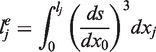
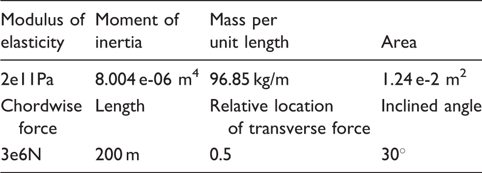
For the cable system shown in Figure 1, the total chord-wise length is l0, the elastic modulus is E, the moment of inertia is I, the mass per unit length is m, the effective cross-sectional area is A, and the inclination angle is θ. The transverse forces divides the cable system into cable segment 1 (from end A to end C with a length of l1) and cable segment 2 (from end C to end B, with a length of l2). The cable bears the chord-wise tension H. To simplify analyses, a chord - horizontal coordinate system (x
j
‐y
j
) of the original cable and a two segment cable is established as shown in Figure 1.
Diagram of an inclined cable segmented by transverse forces.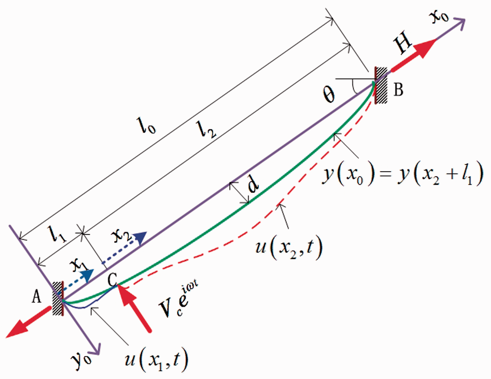
In actual projects, damper type transverse force components only provide transverse disturbance forces to the cable, but do not affect the static configuration, as shown in Figure 1. Discussions in this article are limited to this case. Therefore, the static configuration of a cable can be described by the same second-order parabola function
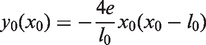
In the equation
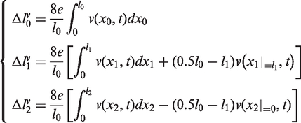
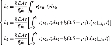
The additional cable tension h
j
is defined as the attached tension induced by the difference between dynamic configuration and static configuration of the cable, which can be calculated by the product of additional strain
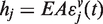
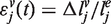
To be approximate, the differential of
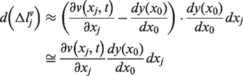
The static configuration of cable is supposed as second-degree parabola
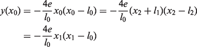
To substitute equation (7) into equation (6), and the integral operation are done in each cable segment, we have
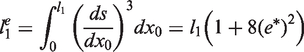
The cable length in static configuration are calculated as following
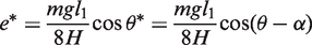
Additionally noticing the geometric relationship of segmented cables in Figure 2, θ* = θ−α. The valid length of cable segment 1 can be expressed as
Schematic diagram of geometric relationship of cable.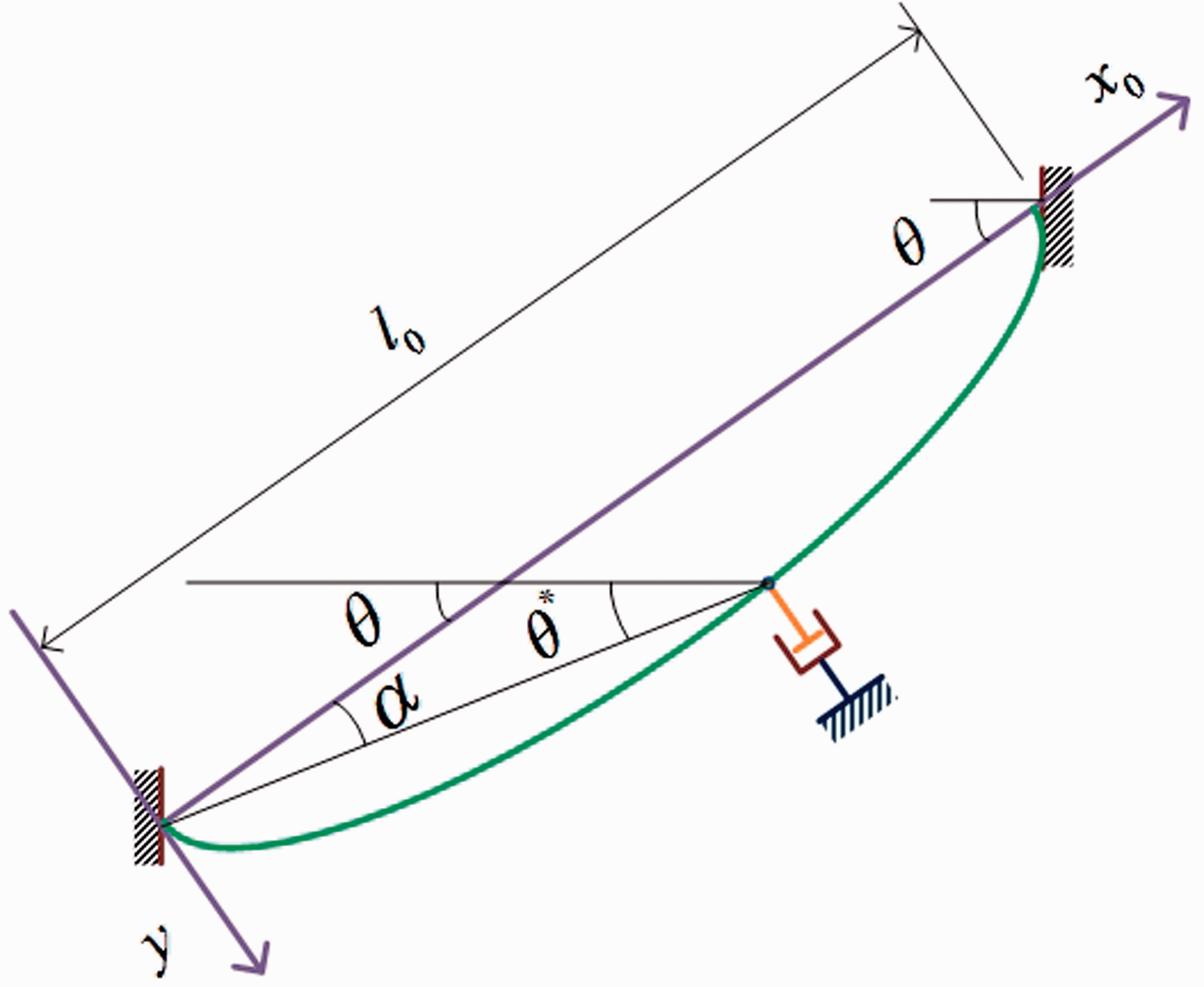
Further note the following relations
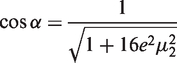
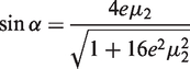
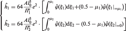
Finally, we get
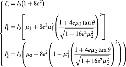
Here, μ1=l1/l0 is the relative location of the transverse force discussed in this article, and μ2=l2/l0 = 1−μ1. And
Substitute equation (5), (8), and (10) into equation (4), we have
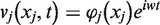
Lets express the transverse displacement as following
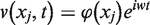
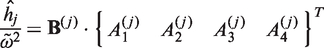
Substitute equation (12) into equation (11), we have

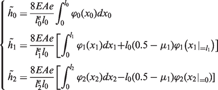
It can be seen from the above equation that when the impact of transverse forces is considered, the calculation equation of the coefficient of additional cable tension is related to the mode shape, the installation height of the damper, and the value of vibration mode function at the position of the damper.
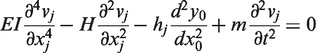
By substituting equations (1), (3) and (13) into the equation (2), the ordinary differential equations of mode shape function ϕ(x
j
) can be obtained, respectively.
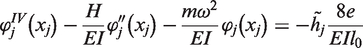
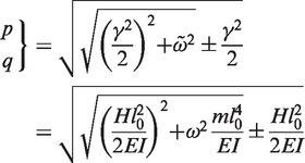
Let
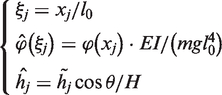
The dimensionless vibration equations of the original cable and two cable segments are as follows

In the equation,
Equation (16) corresponds to the free vibration equation of the cable segment j. Its solution can be expressed by the boundary conditions of the cable or cable segments. Regarding cable segments 1 and 2, the boundary conditions are given by the transverse displacement and rotational angle of points from A, C and B respectively, as shown in Figure 3.
Boundary conditions of cable segments.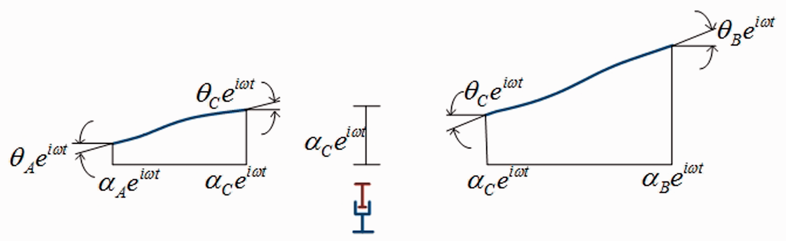
The displacement boundary conditions of the two cable segments are given by the nodal displacement vector of the end of cable segment
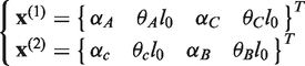
The displacement vector is represented by the dimensionless mode shape function, i. e.
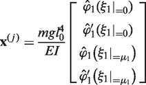
Regarding cable segments 1 and 2, the solutions to the equation (16), the general solution and special solution, is obtained with the boundary conditions of their nodal displacement, which is shown as follows.


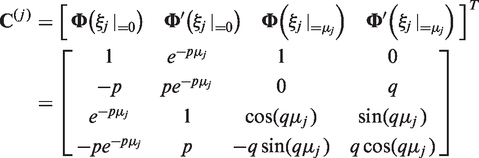
Matrix
The solution of equation (16) can be expressed as following

The non-dimensional form of equation (14) can be rewrite as following
Substitute equation (21) into (22), by reform and transposition, the special solution of the equation (16) can be obtained, as follows
The final solution can be get by merge the general solution and special solution, as present following

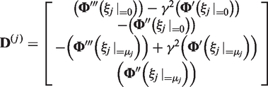
The matrix
The expression of
3. Transverse dynamic stiffness matrix of the cable damper system
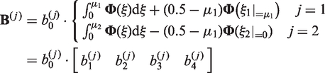
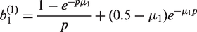
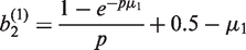
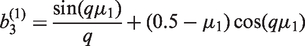
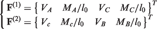
The external forces of the endpoint of two cable segments divided by transverse forces V
c
eiωt are shown in Figure 4, where V
i
is the shear force at end i, and M
i
is the bending moment at end i. The nodal force vector at the end of cable segment is noted as Boundary conditions of cable segment forces.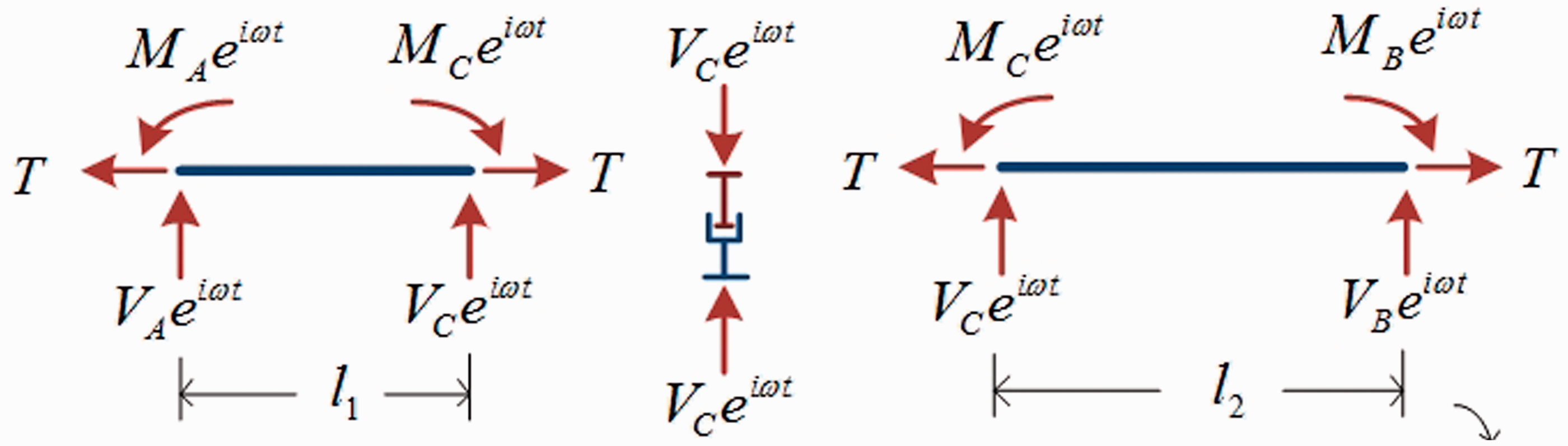
The internal forces in cable segments 1 and 2 can be expressed as follows
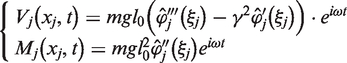
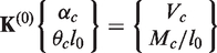
Based on the dynamic equilibrium conditions of internal and external forces, the equilibrium relational expression of the nodal force vector and the nodal displacement vector of cable segment j are given as follows
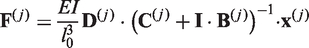
The dynamic stiffness matrix of the cable segment is defined as follows
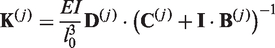
Thus, the dynamic equilibrium relational expression of cable segment j can be written as follows


In equation (30) and (32), due to the limited length of this article, the horizontal stiffness matrix of a cable is given in matrix form, instead of an explicit expression showing matrix elements. However, the derivation process shows that all matrix elements are analytic, meaning a closed form solution will be obtained. The equilibrium equation considers the impact of the bending stiffness, clamped boundary conditions and sag of the cables. The factors considered herein are similar to the cables used in actual projects. Therefore, in theory, this equation can describe the horizontal vibration behavior of cables used in actual projects more accurately.
Similarly, when the impact of sag on cables is not considered, the dynamic stiffness of each cable segment is obtained by letting the matrix
Thus the overall dynamic stiffness matrix of a cable can be solved with the following equation (31). The dynamic equilibrium equation of a cable can be obtained with the following equation (30).
The transverse dynamic stiffness of a single degree-of-freedom of the cable can be transformed from equation (32) to
4. Verification by test
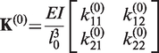
To verify the accuracy of the analytic algorithm for the transverse dynamic stiffness matrix of two degrees-of-freedom of the cable, the data of a vibration test for a full-scale cable damper system were used. The length of the cable used in the test was 170 m, with a diameter of 110.5 mm, a nominal elastic modulus of 2.0 × 10¹¹ pa, and a mass per length unit of 44.07 kg/m. It was fixed transversely in the trough, with both ends clamped and secured. The MR damper was installed at a position 3.4 meters to end of the cable. Artificial excitation was used to record the first order and second order free vibration attenuation under different working conditions of the damper (non-electrified, electrified and under semi-active control). Figure 5 shows the field test.
Full-scale cable test.
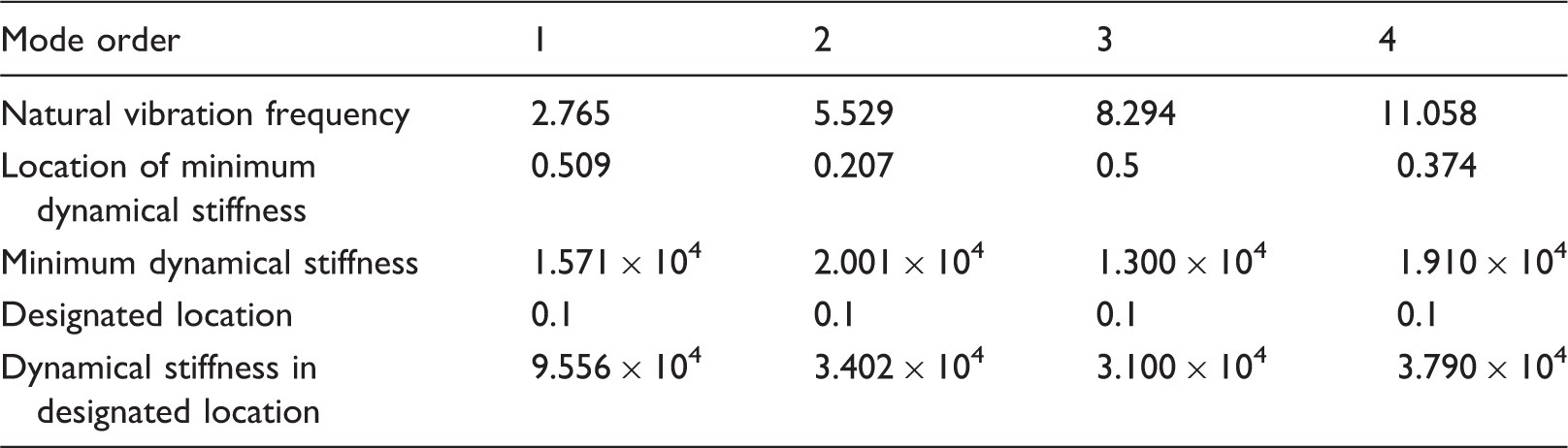
There were 6 working conditions in the test. Figure 6(a) and (c) shows the displacement time history and the damping force time history at the position of the real cable damper. The histories were recorded under two working conditions when the damper is not electrified. The two intervals (within the interval the cable damper is stable) with the logarithmic attenuation rate of time history of the damping force and the displacement time history closest to each other are selected to estimate their continuous peaks and troughs, as shown in Figure 6(b) and (d). By averaging the peak values of damping force divided by the displacement peak value with the lowest phase difference, the measured value of the dynamic stiffness of a cable is estimated. The results are shown in Table 1.
Estimation of time history of excitation and dynamic stiffness of cable. (a,b ) Mode 1 (f = 0.8789) and (c,d) Mode 2 = (f = 1.7578). Comparison of calculated value and measured value of dynamic stiffness. When the logarithmic attenuation rate of the time history of force of the time segment is only 68.2% of the displacement time history, a larger error will be caused.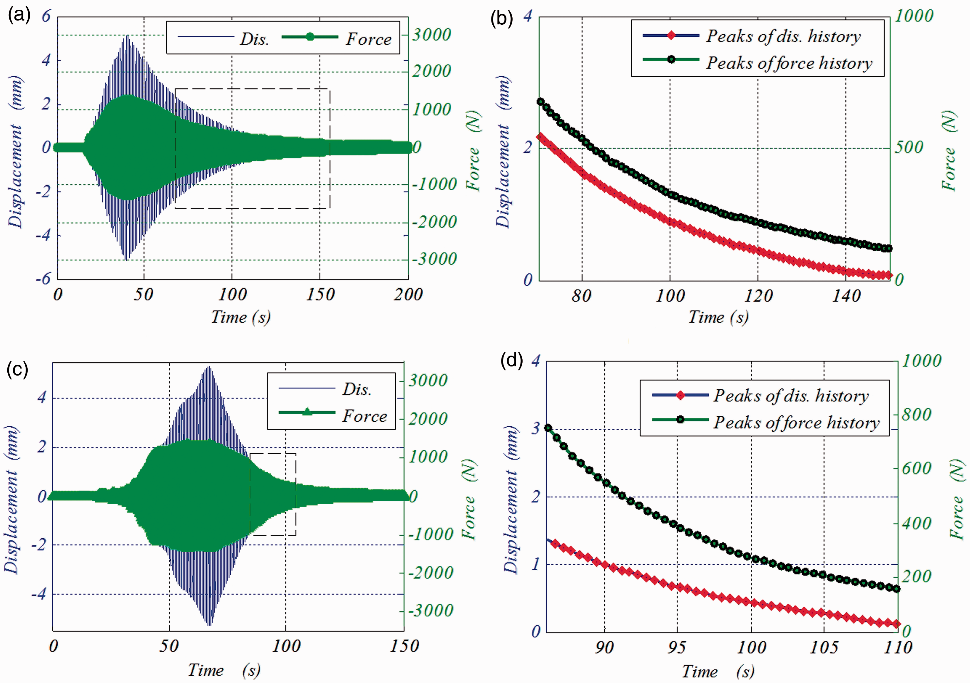
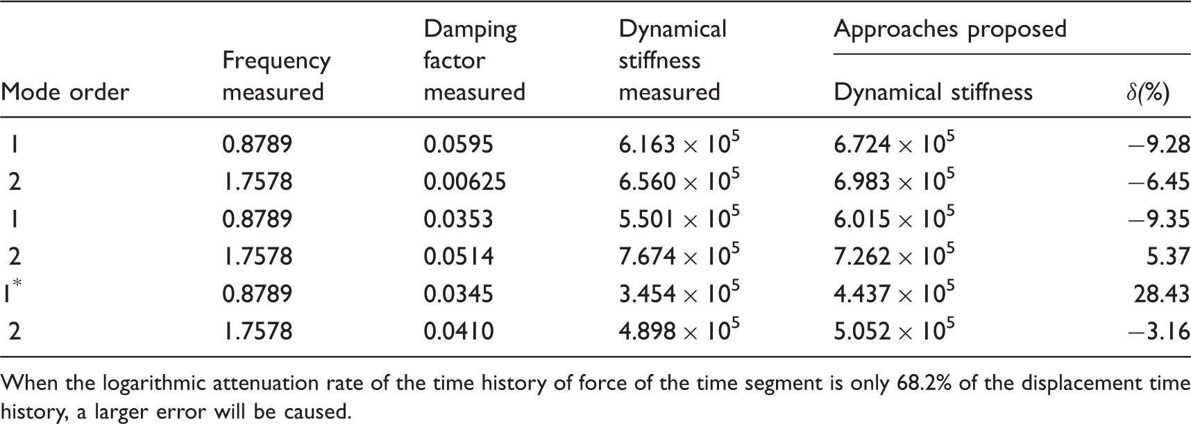
The measured frequency and logarithmic attenuation rate of the selected segment are used to obtain the corresponding complex frequency, by conversion, which is then substituted into equation (28) to calculate the dynamic stiffness matrix of the cable segment, accounting for sag. Equation (31) is used to calculate the total stiffness. Equation (34) is used to obtain the transverse dynamic stiffness of a single degree-of-freedom at the damping location. These results are also in Table 1.
As shown by the values in Table 1, in addition to the 5th working condition, the dynamic stiffness method accounting for sag is correlates closely to the measured values, with the relative error less than 10%. The error of the 5th working condition is larger, reaching 28.43%, mostly due to the poor collaboration between the damper and the cable under the working conditions. It is very difficult to find the time interval of the time history of the damping force closest to the attenuation rate of the displacement time history. Due to the nonlinear properties of the damper itself and the influence of its own stiffness, the estimated values of the dynamic stiffness have a certain disparity with the actual value. This article compares the analytical solution with the measured value to obtain the approximate qualitative solutions, ignoring precision. Overall, the closed form solution results for the dynamic stiffness are reasonable and reliable.
5. Characteristics of the transverse dynamic stiffness of a cable
The transverse dynamic stiffness is very important for the analysis of the vibration of the cable system. By using the dynamic stiffness, the vibration response of the systematic vibration characteristics can be analyzed, and the variation patterns of dynamic stiffness of the cable under complex conditions can be studied. Boundary conditions, inclination angle, bending stiffness, sag and other factors all have varying degrees of influence on the dynamic stiffness. While the cable vibration properties, under the influence of some factors, have been investigated, studies focusing on transverse dynamic stiffness are very rare, especially those considering all the factors mentioned above. Therefore, the algorithm for a closed form solution for transverse dynamic stiffness with a single degree-of-freedom, given by this article, is used to study the distribution pattern of the dynamic stiffness of an inclined cable.
Basic parameters of the cable.
5.1. Variation pattern of the dynamic stiffness of a cable with frequency
Figure 7 shows the distribution pattern of the frequency domain of the dynamic stiffness of a cable at the mid-point and near the ends (μ1 = 0.1, 0.5). The figure shows that the dynamic stiffness in the frequency domain is divided by positive or negative infinity approximately creating discontinuous periodical intervals. When the value of the stiffness approaches positive or negative infinity, in the process, such that a frequency approaches the frequency of a certain order, the node of the mode shape of the order is closest to the point of frequency. The cable gains the greatest amplitude vibrating at the frequency when the dynamic stiffness passes through the zero axes.
Variation of frequency domain of dynamic stiffness of the cable.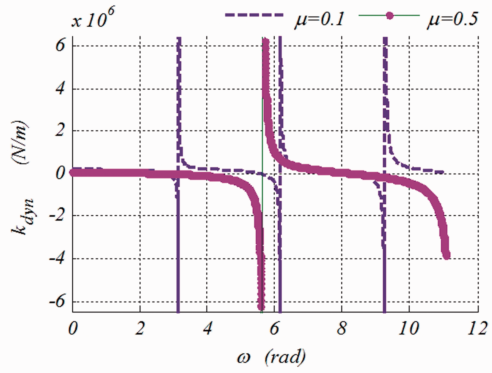
Then the distribution of dynamic stiffness in the complex frequency domain of the midpoint (μ1 = 0.5) of a cable is investigated. Figure 8 shows the three-dimensional dynamic stiffness diagram near the first order vibration frequency of a cable. The horizontal coordinates are composed of the frequency ω and the attenuation factor σ. The height axis signifies the modulus of dynamic stiffness. It can be seen the dynamic stiffness of the midpoint of a cable shows a shape like an inverted cone. The projection of the contour is approximately that of concentric circles in the horizontal plane. The frequency coordinates of the center of the circle correspond to the actual first-order modal frequency. The axis coordinate of the damping factor is zero. The section curve of any frequency or attenuation factor can be described by the quadratic parabola.
Three-dimensional distribution of the complex frequency domain near the fundamental frequency of dynamic stiffness of a cable.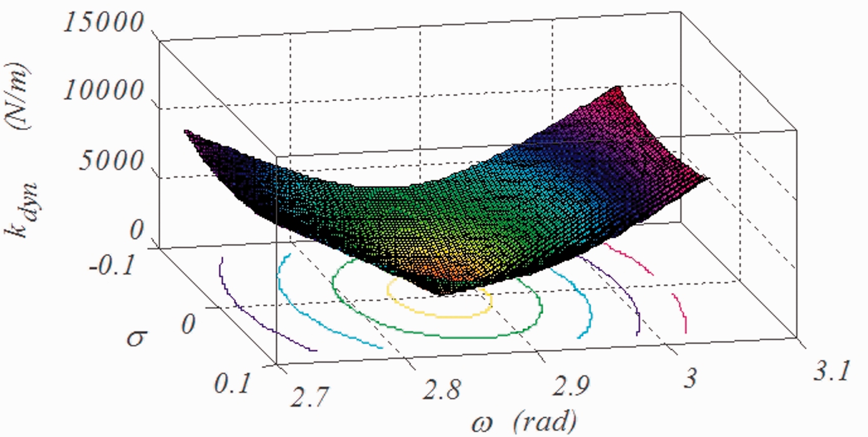
5.2. Spatial distribution pattern of stiffness
In practical engineering, the examination of the spatial distribution of the dynamic stiffness of a cable at specified frequencies is often needed. The spatial distribution of dynamic stiffness is investigated accounting for the estimated value of the fundamental frequency of cable μ1∈[0,1] (given by the taut string formula). Other parameters of the cable are fixed to make the transverse excitation change along the cable length. Figure 9 shows the distribution pattern of the dynamic stiffness along the cable length with the 1st ∼ 4th order frequencies of the cable at the estimated values.
Spatial distribution of each element of the stiffness matrix with the estimated value of fundamental frequency. (a) ω = 2.765, (b) ω = 2.765 × 2, (c) ω = 2.765 × 3, and (d) = ω = 2.765 × 4.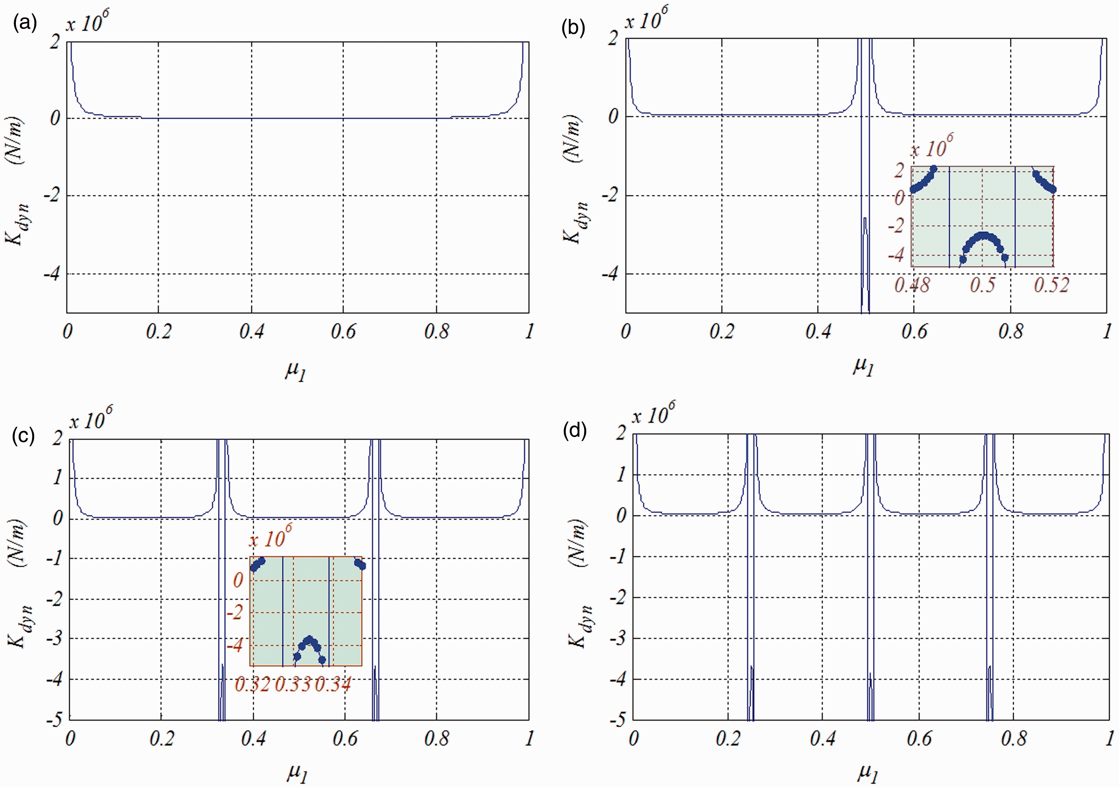
Dynamic stiffness of the first 4 orders of natural vibration frequency (unit: N/m).
5.3. Influence of the major parameters on the dynamic stiffness
In actual engineering projects, values of the transverse force and dynamic stiffness of a cable near the anchorage point are crucial. For this, only the dynamic stiffness near the anchorage of the cable is analyzed in this study. When discussing sag, the dynamic stiffness of the midpoint is also considered.
5.3.1. Inclined angle
The transverse dynamic stiffness given by this article is defined as the direction perpendicular to the tangential direction. Due to the change of the two components of gravity and the geometrical non-linearity of the cable itself, the influence of the inclination angle on the dynamic stiffness cannot be ignored. Figure 10 gives the change patterns of the relative variation of dynamic stiffness δ
k
at the bottom of cable (μ1 = 0.1), with the inclined angle. The dimensionless δ
k
is defined as follows
Variation of the values of the first 6 orders of dynamic stiffness with the inclined angle (μ1 = 0.1).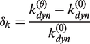
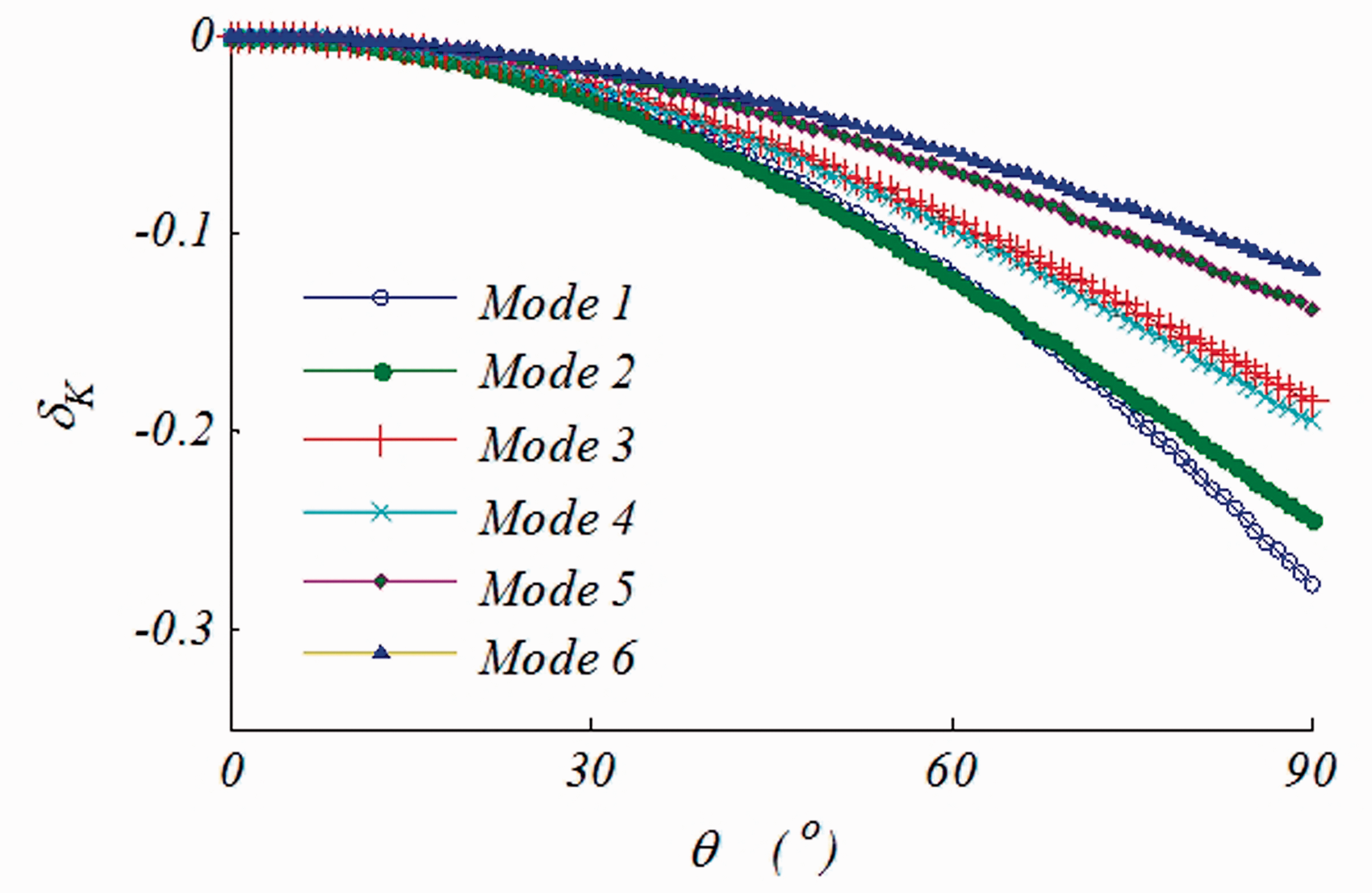
Figure 10 shows, with increasing inclined angle the dynamic stiffness near the end of the cable decreases, the smaller the frequency, the greater the decrease in amplitude of dynamic stiffness. The dynamic stiffness of a cable can reduce by about 27.6% when calculating the first order vibration. The results show that when doing a field excitation on a cable-stayed bridge, a cable which is artificially placed horizontally would contain larger errors. This is required to adjust the working parameters of the vibration exciter according to the inclination situation of the cable.
5.3.2. Bending stiffness of a cable
The influence of the bending stiffness of the cable on the transverse dynamic stiffness is apparent. However, the specific degree of influence needs to be studied further. Similarly, a dimensionless indicator 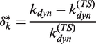
Figure 11 gives the change patterns of Influence of the bending stiffness on the dynamic stiffness of the cable (μ1 = 0.1).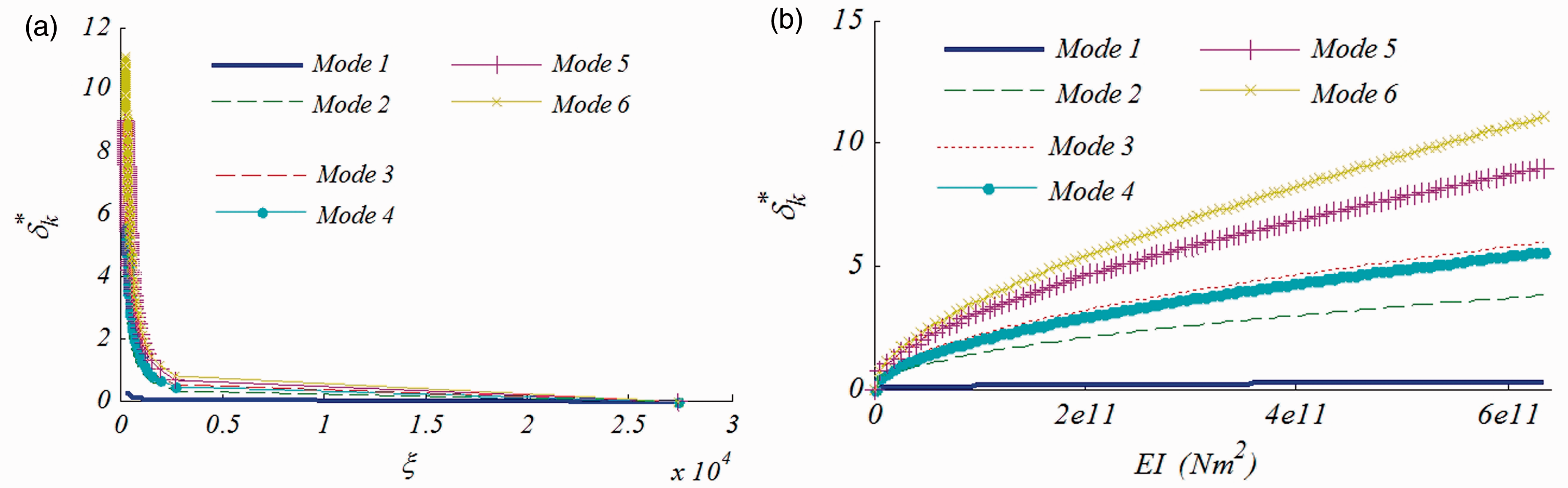
5. 3.3. Effect of sag
The sag of a shallow sag cable, with a value less than 1/8, also has a larger influence on the dynamic stiffness of the cable. When the cable configurations are determined, the sag will only be determined by the tension of cable. To analyze this problem, the basic parameters of the cable are fixed. The sag of the cable is adjusted by tightening or relaxing the cable. The dynamic stiffness of the cable in the 1st–6th order modes, under different sags is calculated, as shown in Figure 12. To compare, the diagram also shows the results of the dynamic stiffness calculation without considering sag.
Influence of sag on the transverse dynamic stiffness. (a) Mode 1 = (μ1 = 0.5, 0.1), (b) Mode 2 = (μ1 = 0.5, 0.1) and Mode 3 = (μ1 = 0.5, 0.1).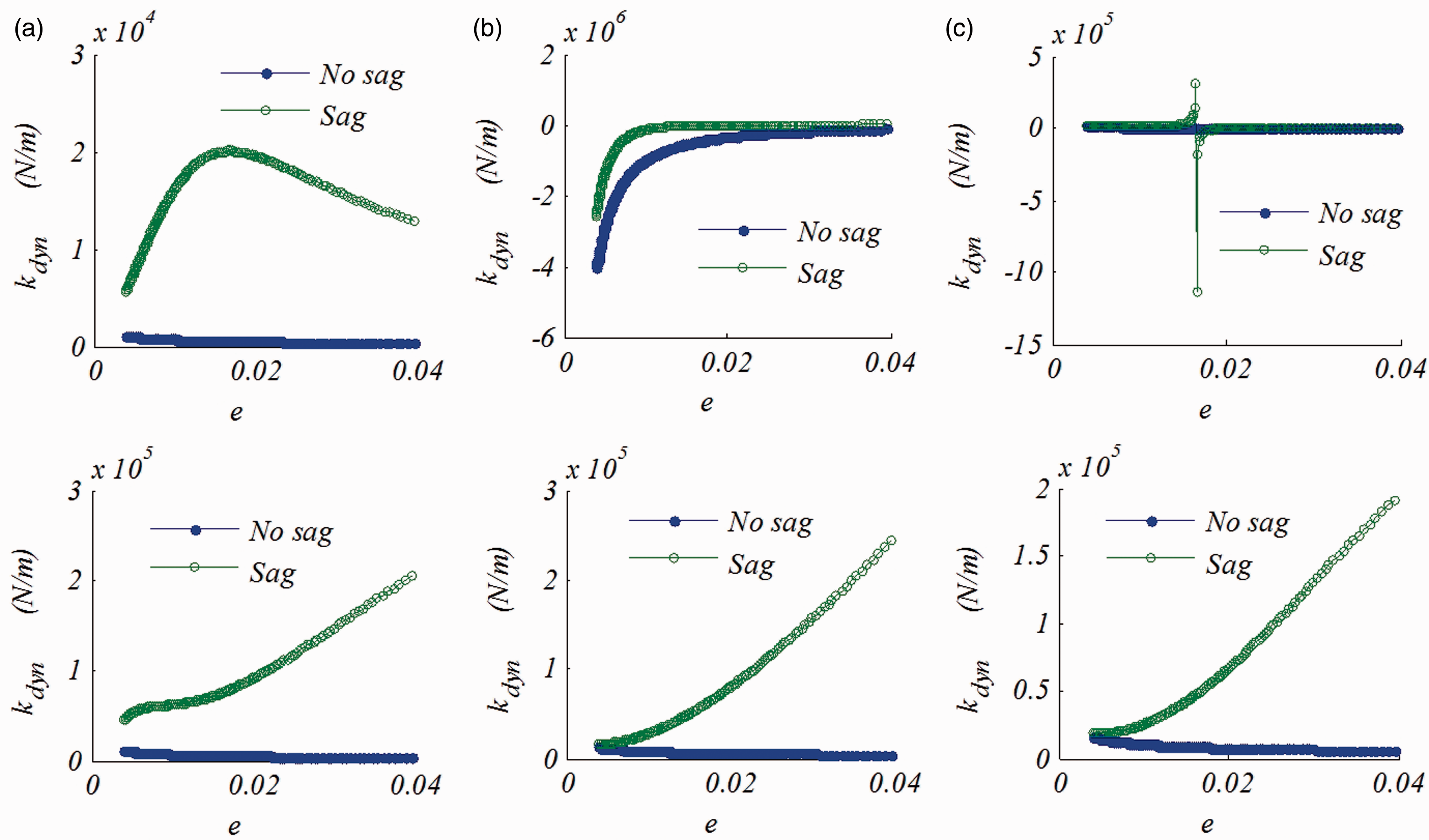
From Figure 12 the influence of the sag-span ratio of the cable on the dynamic stiffness at the anchorage of the cable is very large. With the gradual relaxation of the cable tension, cable sag increases. When considering the effect of sag, the dynamic stiffness of the frequency of each order of the cable, on the ends, increases monotonously. When the effect of sag is not considered, the values from the dynamic stiffness calculation results decrease slightly. They are smaller compared to the dynamic stiffness which considers the effect of sag. The greater the sag, the greater the difference will be.
The variation pattern of dynamic stiffness at the midpoint of the cable is quite different from that on the ends. The influence of sag on dynamic stiffness at the fundamental frequency is larger than that at other orders. With the increase of sag-span ratio, the dynamic stiffness at the fundamental frequency increases initially and then decreases. At approximately e = 0.0165, the peak value appears. At the second order (an even-number order), the curve of the dynamic stiffness tends to slow, regardless of sag consideration. This suggests that the influence of sag gradually decreases, which correlates with conclusions from previous literature. At the third order, a similar conclusion is obtained. However, a sudden change occurs at the point with the same sag-span ratio e = 0.0165. The reason for the occurrence of such an abrupt change may be related to the passover and curve veering of frequency in the process of cable relaxation. This phenomenon is worth further study.
6. Conclusion
Transverse dynamic stiffness is a powerful tool for the vibration analysis of cables. Although the transverse dynamic stiffness of cables is expressed by a matrix or matrix element in this article, all the intermediate variables for the derivation process can be written in the form of an elementary function. Therefore, the dynamic stiffness we obtain is a closed-form solution. Through a full-scale cable test with the damper, the reasonability and reliability of our method is verified.
The closed-form solution accounts for all the factors except for the internal damping of the cables. Theoretically, the solution in this study has a high precision. Through the analysis of the transverse dynamic stiffness of cables, a complex distribution pattern is revealed in terms of both the frequency domain and in space. Other factors, including inclination angle, flexural stiffness and the sag of cables also have large influence on the dynamic stiffness of cables. Instead, if the ideal taut string theory is adopted, cable sag is neglected, or the inclined cable is approximated to be horizontal, the results will have considerable errors and an erroneous conclusion may be drawn. Therefore, all these factors must be considered. This demonstrates the significance of our method.
Footnotes
Funding
Supported by the State high-tech research and development plans (863), grant no. 2014AA110402, State Meteorological Administration Special Funds of Meteorological Industry Research (grant no. 201306102), the Project of National Key Technology R&D Program in the 12th Five Year Plan of China (grant no. 2012BAJ11B01), National Nature Science Foundation of China (grant no. 50978196), Key State Laboratories Freedom Research Project (grant no. SLDRCE09-D-01), The Fundamental Research Funds for the Central Universities, and State Meteorological Administration Special Funds of Meteorological Industry Research (grant no. 201306102).