
Abstract
Industrial processes are becoming increasingly complex, requiring advanced modelling techniques to understand their behaviour and improve their performance. In this context, deep learning algorithms have proven to be effective tools for modelling dynamic systems, with Recurrent Neural Networks (RNNs) being particularly suitable for time-series data. However, the computational complexity of deep learning models can be a limitation in industrial environments, where real-time responses are required.
This work proposes the use of Deep Echo State Networks to model an industrial system. The aim is to evaluate its performance in real-time industrial applications when running on embedded devices. The approach is validated on a process composed of four interconnected water tanks, which exhibits typical nonlinear industrial dynamics. Among several candidate architectures (including vanilla RNNs or LSTMs), Deep ESNs were selected for their balance of accuracy and computational efficiency. Different input-output setups and number of Deep ESN layers are tested, and results are compared with LSTMs in terms of accuracy and execution time. Finally, the best Deep ESN models are implemented on industrial embedded devices to evaluate the possibility of running these models in real time.
The proposed approach achieved up to a 33% reduction in RMSE and a 14% improvement in
Introduction
Industrial processes tend to become increasingly advanced and complex, and this complexity implies greater difficulties in their management and monitoring. For this reason, modelling industrial systems is a task of great relevance to better understand its characteristic behaviour and how it evolves over time. In addition, having a model of the system also facilitates the detection of failures or scenarios that deviate from normal behaviour, allowing operators to take action to correct these problems. Eventually, this modelling leads to more detailed analyses that allow the process to be optimised, leading to improved performance and greater efficiency, thereby reducing energy consumption and increasing production. 1
However, the modelling and representation of dynamical systems in an industrial environment presents certain difficulties: it is common to have a large amount of data extracted from processes that change in a matter of milliseconds, but extracting knowledge about the process behaviour from this data is not as easy as it may seem. 2 For this reason, it is important to obtain a model that is as close as possible to the reference industrial process, which allows the dynamics of the system to be represented as faithfully as possible.
In this respect, although there are different approaches to develop such models of physical systems, machine learning tools are one of the most widely used. Among the various machine learning algorithms available, Recurrent Neural Networks (RNNs) have proven to be particularly effective in modelling dynamic systems, especially those that involve temporal sequences. 3 RNNs distinguish themselves from other neural networks by their unique architecture, which includes recurrent connections to capture past dependencies across time steps. This architectural feature allows RNNs to model sequential data with high-dimensional hidden states, while efficiently handling non-linear and complex dynamical behaviours that arise in time-series data. 4 Recent applications demonstrate the successful use of spatio-temporal deep learning networks in dynamic prediction tasks, such as lightning nowcasting, 5 which reinforce the relevance of such models for real-world sequence modelling under uncertainty.
Within machine learning, deep learning has emerged in recent years as a very powerful tool for modelling complex systems, mainly due to its ability to capture non-linear patterns and relationships in data. 6 Deep learning is based on the use of multi-layer neural networks, which allow features to be extracted from the input data at different levels of abstraction. This has enabled its application in dynamic system modelling under uncertain or complex conditions, such as vehicle dynamics in snowy environments, 7 real-time fault diagnosis in industrial systems, 8 and efficiency improvements in automated manufacturing. 1 Furthermore, comparative studies have shown the effectiveness of deep learning techniques in high-dimensional, time-sensitive domains like media content classification, 9 cardiac condition detection, 10 and energy monitoring, 11 reinforcing its generalisability in safety-critical or resource-constrained scenarios.
However, the use of increasingly complex architectures also implies greater computational complexity, requiring more powerful hardware platforms and longer training times. 12 Despite this, with improvements in workload distribution and the use of Graphics Processing Units (GPUs), the training and execution times of deep learning models have been significantly reduced, allowing their deployment in real-time applications across a variety of industrial domains. 13
Nevertheless, the use of such deep learning models in industrial environments can be challenging, especially where computational or hardware resources are limited, and where real-time responses are required to promptly detect anomalies and take action. This has motivated research into lightweight and efficient modelling techniques capable of running on embedded platforms while maintaining predictive performance.1,8
A particularly interesting and valued algorithm in this respect is Long Short-Term Memory (LSTM), a type of recurrent neural network that has proven effective in modelling dynamic systems, particularly in time series prediction. 14 However, despite their modelling capabilities, LSTMs often suffer from slow convergence and training instability.
As an alternative, Reservoir Computing (RC) has gained attention due to its much faster and more efficient training with lower hardware requirements. This is accomplished by generating a hidden layer of recurrent neurons, called the reservoir, that is randomly initialised and held fixed during training, and a linear output layer that is trained under supervision. 15 Approaches such as adaptive reservoir computing have already demonstrated success in manufacturing environments, 16 reinforcing the suitability of this paradigm in industrial contexts.
Among RC models, the Echo State Network (ESN) stands out for its simplicity and effectiveness in modelling complex systems. Moreover, ESNs allow for model adaptation by retraining only the output weights, avoiding full retraining of the model. 17 More specifically, with the introduction of Deep Echo State Networks (Deep ESNs), 18 reservoir computing has merged with deep learning paradigms to build hierarchical architectures of multiple reservoir layers. These models outperform standard ESNs by capturing temporal dependencies at different time scales, 19 and have shown promising performance. Their architecture allows them to efficiently model multi-scale industrial dynamics while avoiding the high training cost of backpropagation-based models.
The lightness, efficiency, and adaptability of standard ESNs and Deep ESNs make them particularly attractive for industrial system modelling, especially in scenarios requiring embedded real-time implementation. Although some studies have explored the application of ESNs in industrial contexts, many focus on simulated or lab-scale systems, 20 and there remains a gap in evaluating their performance on real-world industrial setups. This work aims to help address this gap and contribute to ongoing efforts in the community to develop scalable, low-complexity solutions for industrial modelling.
For these reasons, the application of Deep ESN to the modelling of real industrial systems, and especially the possibility of running these models on low-cost embedded devices, is an interesting and promising field of study that can be useful for improving these industrial processes.
In this context, this work proposes the application of Deep ESNs to model a real industrial process composed of four interconnected tanks, while assessing the feasibility of deploying these models on embedded platforms. Building on previous work, 21 this study extends the evaluation to the complete system, systematically comparing input/output configurations and Deep ESN architectures to determine the optimal setup for accurate and efficient real-time modelling.
Furthermore, a performance comparison of the Deep ESN and LSTM models is performed in terms of accuracy and execution time with the selected best configurations, to evaluate the efficiency of the proposed approach. LSTM models are selected for comparison because they are among the most widely used RNN-based methods for time series modelling, and have shown strong performance in various dynamic system applications. Additionally, previous studies have compared ESNs and LSTMs, highlighting their differences in terms of computational efficiency and prediction accuracy. 22
Finally, the selected Deep ESN models are implemented on low-cost industrial embedded devices to evaluate the possibility of running these models in real time.
This work is structured as follows: Section 2 provides an overview of Deep Reservoir Computing techniques, focusing on Deep Echo State Networks. Section 3 outlines the methodology to implement the Deep Reservoir Computing models, including the selection of the best architectural setups, the comparison with LSTMs and the testing on embedded devices. Section 4 describes the quadruple-tank industrial plant used in the experiments, detailing the different operating scenarios considered. Section 5 presents the results obtained from the experiments conducted with the proposed methodology. Finally, Section 6 summarises the main conclusions of the work and outlines future research directions.
Deep reservoir computing
Reservoir Computing (RC) is a machine learning paradigm that has gained popularity in recent years due to its ability to model complex dynamical systems. RC is based on the concept of a reservoir, a high-dimensional dynamical system that processes input signals and generates a rich representation of the input data. The reservoir is a randomly generated network of interconnected nodes, which are typically sparsely connected and have fixed weights. The input data is fed into the reservoir, and the reservoir’s dynamics transform the input data into a high-dimensional representation, which is then used to predict the output of the system. This projection maps temporal patterns into a geometric space where they become more linearly separable. The output is then generated by a linear readout layer that maps the reservoir’s high-dimensional representation to the desired output. The key advantage of RC is that the reservoir’s dynamics are fixed and do not need to be trained, which simplifies the training process and makes these models more robust to noise and perturbations.
Echo State Networks (ESN),
23
constitute a particular implementation of Reservoir Computing. ESNs rely on a fixed, randomly initialised reservoir and a trainable readout layer. For this reason, ESNs offer an efficient and effective alternative to traditional RNNs,
18
as they are easier to train and require fewer parameters. The reservoir acts as a non-linear, high-dimensional dynamical system, which maps an input vector
The most common variation of this architecture incorporates a leaky integrator mechanism to modulate the recall of previous states.
24
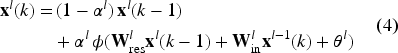
This variant, known as Leaky Integrator ESN (LI-ESN), is the one used in this work and it responds to the following state equation:
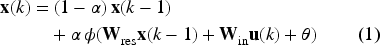
In this equation,
The readout mechanism translates the reservoir states into an Structure of a shallow ESN.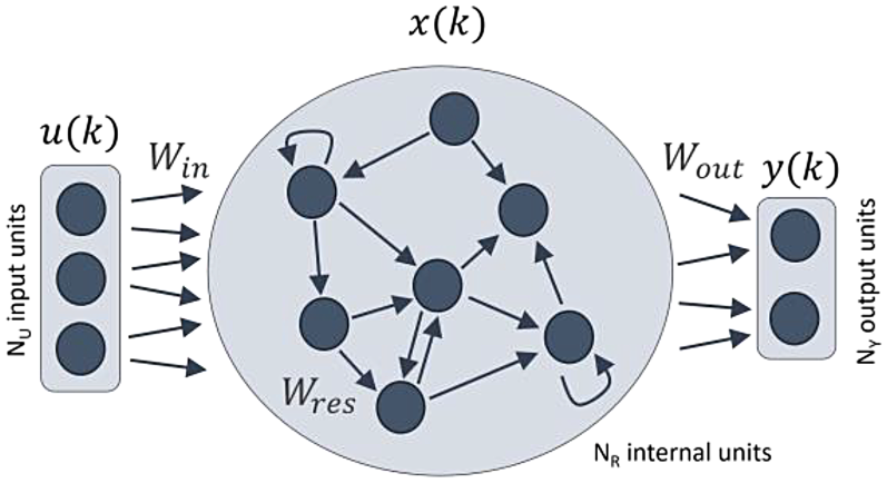

The Shallow ESN architecture is depicted in Figure 1, where bias terms have been omitted for clarity. This structure is composed of three main layers: the input layer, the reservoir layer, and the readout or output layer.
The input layer, parameterised by the weight matrix
The weight matrices
When the reservoir processes an input sequence
There are some variations of the presented Shallow ESN model, such as including
In contrast, the Deep ESN architecture, which was introduced in Gallicchio et al., 18 comprises multiple reservoir layers arranged sequentially: the first reservoir directly processes the input vector, while each subsequent reservoir takes as input the state vector produced by the preceding layer. The architecture of a Deep ESN is depicted in Figure 2. This hierarchical structure allows the network to capture complex temporal dependencies across different time scales, enhancing its ability to model complex dynamical systems.
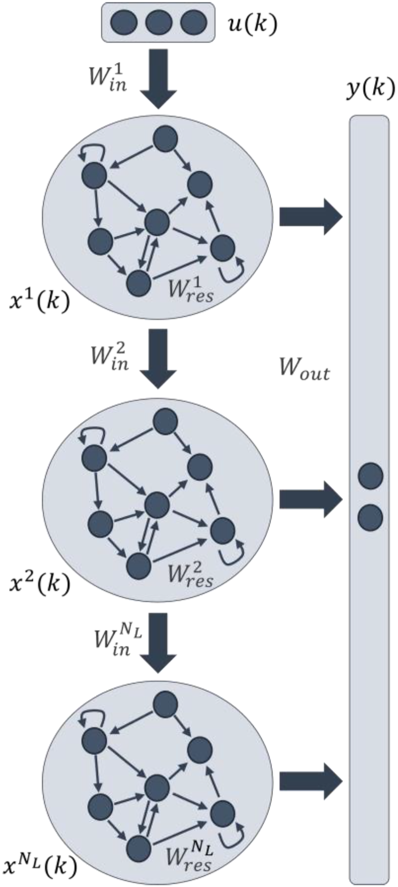
Structure of a deep ESN.
Typically, all reservoirs in the architecture are designed with the same number of units, denoted as
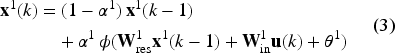
In these two formulas,
Although Deep ESNs add hierarchical structure, they share key operational mechanisms with Shallow ESNs: the weight matrices of all the reservoirs are initialised with random values drawn from a uniform distribution (e.g.,
For producing the output of the network, the most common approach is to link the states from all reservoir layers to the readout. This configuration, illustrated in Figure 2, computes the output as a weighted sum of the states from all layers, as described by the following equation:
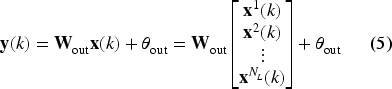
In this equation,
Deep ESNs offer several notable advantages compared to Shallow ESNs. These key benefits are detailed in Gallicchio et al., 29 and are briefly outlined as follows. Firstly, Deep ESNs provide a hierarchical structure that enables the modelling of multi-scale temporal dynamics across layers, with higher layers typically exhibiting slower dynamics. Additionally, given the same total number of reservoir units, Deep ESNs have a greater memory capacity, enabling them to capture and utilize information from earlier inputs more effectively. Another benefit is that distributing the reservoir units across multiple layers decreases the number of non-zero recurrent connections, improving computational efficiency. As a result, for a fixed total number of units, Deep ESNs can achieve significantly better performance than Shallow ESNs.
This section describes the proposed steps to implement Deep Reservoir Computing for modelling an industrial process. This implementation approach addresses specific industrial requirements: compared to conventional deep learning, it offers reduced training and deployment time, real-time operation capabilities with reduced inference times, and hardware compatibility through optimized deep structures for low-cost embedded devices. These features make the solution suitable for industrial automation, where cost, timing precision, and rapid deployment are critical.
The implementation process starts with the selection of the best Deep RC architectural setup to address different operational scenarios in the modelled industrial system. The next step is to evaluate the performance of the best setups on their own and against LSTM reference models. Finally, the selected setups are implemented on embedded devices.
Selection of the best deep architectural setup
To begin with, based on the industrial process to be modelled, different operating scenarios and various configurations of inputs and outputs are defined for the models. These scenarios and input and output configurations are defined according to the characteristics of the industrial process, taking into account the variables of interest and the modelling objectives. Once the scenarios and the input and output configurations of the models have been defined, the first step for the RC implementation is the selection of the best architectural configuration for each of the scenarios and tanks.
The key design consideration for the Deep RC architecture is determining the optimal number of reservoir layers. In addition, other hyperparameters have to be selected in order to generate a faithful model. For this purpose, the performance of the Deep ESN models is evaluated with different numbers of reservoir layers. The aim is to have the performance defined as a function of the number of reservoir layers, thus analysing the performance improvement when adding more reservoir layers to the ESN setup.
The Deep ESN selection process is structured as show in the algorithm:
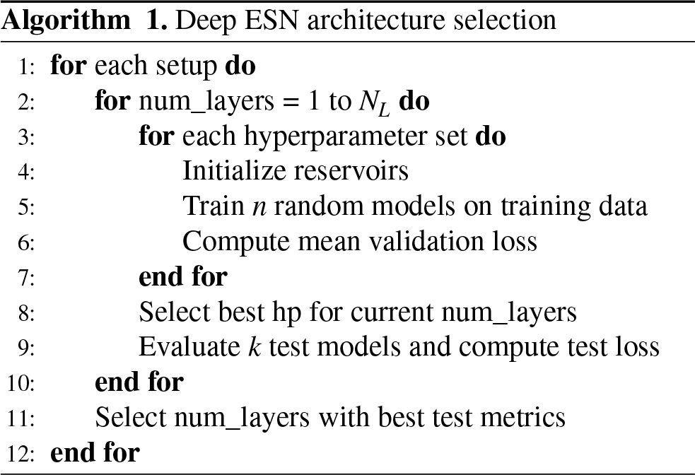
First, for each of the previously defined architectural setups, a list of numbers of layers to test is selected, e.g. from 1 to 10 layers. Then, for each number in the range, a search for the best hyperparameters is performed on the training and validation data. When the number of reservoir layers in the model is more than 1, the reservoirs in the different layers are initialised with the same hyperparameters but with different random seeds. Taking into account the randomness involved in ESNs, different models are generated for each set of hyperparameters tested, to make a more objective assessment and to consider the mean of the losses obtained in the validation data.
In order to compare the models, regardless of the number of layers, the total number of internal units in the reservoirs is kept constant and evenly distributed across all layers as more layers are added. For example, if a model is defined with 1000 internal units, with 4 layers each layer will have 250 internal units and with 8 layers each layer will have 125 internal units.
Once the best hyperparameters are found according to the lowest loss on validation data, some new random models are trained with the best parameters, and then the performance of each new model is evaluated on the test dataset. After testing different numbers of layers and getting the mean test loss for each one, the best Deep ESN model is selected based on the calculated metrics: the model with the number of layers that generates the least error.
The selection process is then repeated for each of the defined architectural setups. The aim is to find the best Deep ESN setup for each of the tanks, that is, the setup that generates the best performance for the upper tank and the lower tank. The selected setups and the best number of Deep ESN layers in these setups are the ones that will be used in the next steps of the implementation process.
All the ESN models are implemented using Python library ReservoirPy,
30
which allows the user to configure and parameterise the different elements of an ESN (input, reservoir, readout
Performance evaluation against LSTM
Once the best Deep ESN setup has been selected for each of the tanks, the next step is to evaluate the performance of the selected models against a reference model. In this case, the reference model is a Long Short-Term Memory network, as it has proven to perform quite well in time series prediction tasks. The evaluation and comparison process is assessed taking into account the following aspects:
Training time: time required to train the model with a defined trained dataset. Sample prediction time: mean time required to predict each of the steps in the time series. Performance loss metrics.
The aim is to evaluate how ESN improves efficiency over LSTM, not only in terms of performance metrics, but also in terms of training time requirements and prediction speed, which are crucial for real-time applications. In this case, both Shallow ESN and Deep ESN are included to further compare the improvement between both architectures and LSTM.
The widely used Python libraries TensorFlow 31 and Keras 32 are selected for the implementation of the LSTM models, These libraries allow the user to define and parameterise the different elements of a LSTM model. The optimisation of the models is performed with Adam algorithm.
Deep RC on embedded devices
The final step in the implementation process is to deploy the selected Deep RC models on embedded devices with limited computational resources in order to evaluate these models in real-time industrial applications. The evaluation will take into account the following aspects:
Training time: the time required to train the model with a defined training dataset. Dataset prediction time: the time required to predict the whole test dataset. Sample prediction time: the mean time required to predict each of the steps in the time series.
In this work, three different embedded devices were selected: a Raspberry Pi Zero 2 W, a Magelis IIot Core Box from Schneider Electric, and a Simatic IoT2050 from Siemens. All of these IoT devices share the same 1GHz quad-core Arm Cortex-A53 CPU, but have different amounts of RAM and other hardware variations. The Raspberry Pi Zero 2 W is a low-cost device easily accessible for all users which has 512MB of RAM. The Magelis IIot Core Box is a more powerful device designed for edge computing tasks in industrial environments, with 1GB of RAM. Finally, the Simatic IoT2050, also designed for industrial IoT tasks, is a device with 2GB of RAM. The local PC used for hyperparameter search, evaluation and model selection tasks has a 3.4GHz seventh-generation Intel Core i5 processor and 8GB of RAM.
Experimentation system
This section provides a description of the experimental environment used in this work. In addition, the different operating scenarios considered for the four-tank system are detailed, as well as the different setups for the Deep ESN models that will be evaluated. Finally, the datasets used to work with the plant are described.
Description of the four-tank system
The experimental setup, located at the Remote Laboratory of Automatic Control at the University of León, consists of a real industrial implementation of the well-known four-tank system, initially proposed by Karl Henrik Johansson. 33 The industrial plant used for this work and its schematic representation are shown in Figure 3.
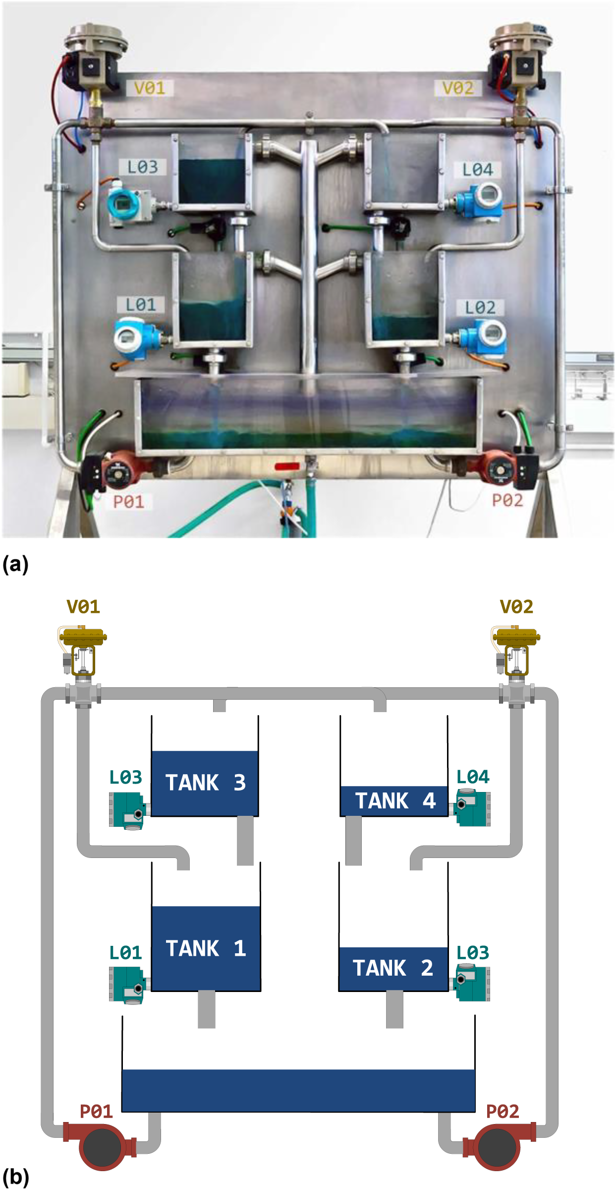
Industrial plant and its diagram. (a) Industrial plant used and (b) Industrial plant diagram.
This plant is composed of four water tanks arranged in two vertical pairs. Water is supplied to the four tanks from a lower reservoir tank using two twin centrifugal pumps controlled by variable frequency drives, generating a multi-level control scenario. As the water leaving an upper tank feeds the one immediately below it, the level in the latter depends on the level in the former, creating a set of interconnected dynamics.
The water driven by the pumps is distributed to the tanks by means of two three-way pneumatic valves, so that each pump-valve set delivers water to two of the four tanks. In addition, the valves and tanks are cross-connected so that each valve supplies water to the adjacent lower tank and the opposite upper tank.
This configuration creates a complex and interdependent control system, where the water levels in the lower tanks are affected not only by the pumps and valves but also by the interactions with the other tanks. Finally, to measure water levels, each tank is equipped with a pressure sensor at the base. Table 1 outlines the main inputs and outputs of the plant that will be used for the models.
The mathematical representation of the four-tank process is derived from the fundamental principles of fluid dynamics, namely Bernoulli’s principle and the mass balance law. These principles lead to a set of differential equations that describe the evolution of water levels in each tank over time. To model the system’s behaviour, a state-space representation is employed, which is widely used in control engineering due to its ability to capture the dynamic relationships between system variables.
However, translating this theoretical model into a physical industrial setup introduces real-world complexities. This system was specifically selected because it encapsulates several common challenges in industrial environments, such as nonlinear dynamics, measurement noise, dead zones, and actuator asymmetries. These factors lead to discrepancies between the theoretical model and actual behaviour, reflecting conditions typically found in industrial automation scenarios. As such, the four-tank system serves as both a controlled experimental platform and a representative proxy for real industrial processes. Addressing its complexities requires advanced modelling techniques, such as machine learning approaches, that can better capture and compensate for nonlinear behaviours, overcoming the limitations of traditional linear control methods.
The four-tank plant as a whole operates as a multivariate control system, where pumps (P01, P02) and valves (V01 and V02) are the input variables, and the desired water levels in each tank (L01, L02, L03 and L04) are the output variables. Therefore, the first option considered is to model the entire plant as a single system, where the inputs are the pumps and valves and the outputs are the levels of the tanks. This configuration is called
However, defining a single model of the whole process that performs well in all circumstances is not that straightforward, as it implies greater complexity and difficulty. It is therefore proposed to divide the process into different subsystems, each focused on predicting the level of a reservoir. This allows the models developed with these subsets to be compared with the single model of the whole plant, to see which of them gives better results.
By considering the system in terms of different subsystems, it is possible to work with different operating scenarios depending on which system inputs are operating at any given time. Thus, if each pump-valve set is considered as a single input or source of water flow, two main different operating scenarios can occur in the four-tank process: if only one pump and one valve are activated, a Single Input-Single Output (SISO) scenario occurs, while if both pump-valve sets are activated, a Multiple Input - Multiple Output (MIMO) scenario occurs.
In this work, therefore, apart from the whole setup 4-TANK it is proposed to work with a SISO-type scenario and a MIMO-type scenario, defining different setups in both scenarios. Assuming a symmetrical plant configuration, with two separated sets of two tanks connected in series (tank 3 and tank 1, tank 4 and tank 2), the set of tanks 3 and 1 is considered as a reference for this work, with tank 3 being chosen as the upper tank and tank 1 as the lower tank. The focus of this paper is therefore to find the best Deep RC setup for modelling the upper and lower tanks in these scenarios, selecting the setup that has the best performance for each of them.
Firstly, Figure 4 shows the scheme of the four-tank system considered for the SISO scenario, where tank 3 is the upper tank and tank 1 is the lower tank. In this scenario, there is an upper tank that can be supplied with water by the opposite pump-valve set (in this case P02 and V02) and a lower tank that receives the water discharged from the upper tank. This is the scenario that was the subject of the Deep ESN work previously developed with the four-tank system.
Variables of the quadruple-tank process.
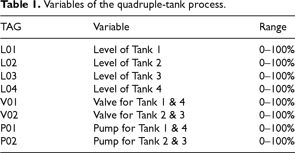
Variables of the quadruple-tank process.
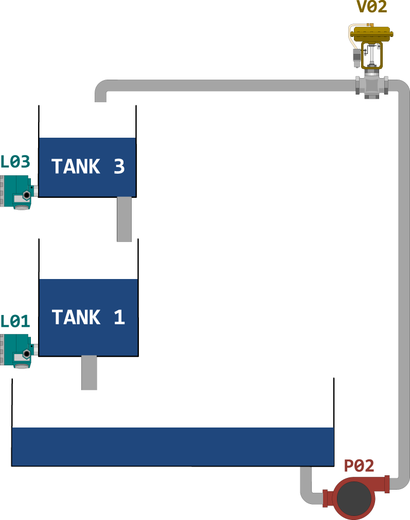
SISO scenario for the four-tank system.
In the SISO scenario, the modelling of the upper tank is more straightforward: the process inputs that influence the tank level, to be used as model inputs, are the pump P02 and the valve V02, while the output is the tank level L03. In this case, the setup of inputs and outputs considered is called
In contrast, the modelling of the lower tank is more complex, as the level of tank L01 depends on the level of the upper tank L03 and, consequently, on the system inputs P02 and V02. Therefore, two different configurations have been considered for the lower tank in the SISO scenario, one using the level of tank L03 as model input, called
Secondly, Figure 5 shows the scheme of the four-tank system considered for the MIMO scenario, where tank 3 and tank 1 are again the upper and lower tanks, respectively. In this scenario, the upper tank is again supplied with water by the opposite pump-valve set (P02 and V02), and the lower tank that receives the water discharged from the upper tank and also the water from the adjacent pump-valve set (P01 and V01).
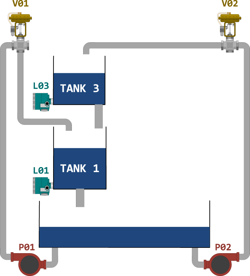
MIMO scenario for the four-tank system.
As it can be observed in the figure, the model for the upper tank is analogous to that defined in the SISO scenario, with identical inputs influencing the level of the tank. Therefore, the setup for the upper tank in the MIMO scenario can be replicated as in the SISO scenario,
The modelling of the lower tank is more complex than in the SISO scenario: the level of tank L01 depends on the level of the upper tank L03 and thus on the system inputs P02 and V02; but it also receives the flow from the adjacent pump and valve (system inputs P01 and V01). Therefore, two different setups are considered for the lower tank, one using as inputs the upper level L03 together with the pump P01 and the valve V01, called
Table 2 summarizes the input and output configurations for each of the evaluated setups. These setups can be organised depending on the tank level to be modelled as follows:
Definition of the different architectural setups to evaluate.
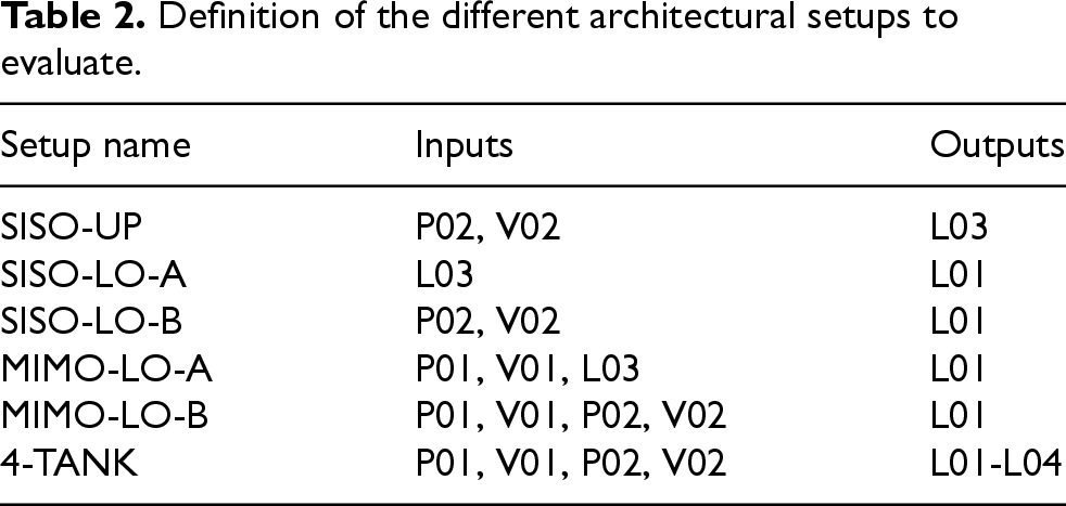
To predict the level of the SISO-UP 4-TANK SISO-LO-A SISO-LO-B 4-TANK MIMO-LO-A MIMO-LO-B 4-TANK
To predict the level of the
To predict the level of the
The datasets used in this work were obtained from the controller of the quadruple-tank system, where the water levels in the tanks and the pump and valve settings were recorded. Two different datasets were defined and captured: one for the SISO scenario, with just pump P02 and valve V02 connected, and another one for the MIMO scenario, with both pumps and valves working.
For both scenarios, the system operates in a closed-loop control mode with pumps as actuators to avoid saturation of the tanks and to maintain the water levels within the desired setpoints. Random setpoints for the levels and random opening percentages for the valves were therefore defined every 60 seconds, assuming that this would be sufficient time for the water levels to reach the steady state.
Both datasets were collected for 24 hours each one, with a sampling rate of 100 milliseconds. The datasets were then resampled to 5 seconds to obtain a better performance with the designed models, based on the previous works with the four-tank system. 21 The datasets were then divided into three parts: training, validation, and test, with a ratio of 60%, 20% and 20% respectively.
Results
This section presents the results obtained from the implementation of the Deep RC models on the four-tank industrial process. The results are structured in three main sections: the selection of the best Deep RC architectural setup, the comparison of the selected models with LSTM reference models, and the implementation of the selected models on embedded devices.
Selection of best the architectural setup
The selection of the best Deep RC architecture is based on the performance of the models with different numbers of reservoir layers. More specifically, the models are evaluated with a range of layers from 1 to 10, and the performance is calculated for each number of layers on the test dataset, in terms of the Root Mean Squared Error (RMSE) and the Coefficient of Determination (
The hyperparameters of the Deep ESN models are selected from a range of values, as shown in Table 3, using a random search algorithm. Thus, at each iteration, a set of hyperparameters is randomly selected from the defined ranges, and the model is initialised with these hyperparameters. As it is known that the performance of an ESN model improves with a larger number of reservoir internal units, this parameter is left fixed and limited to
Tested ranges of ESN hyperparameters and best options selected for SISO and MIMO scenarios.
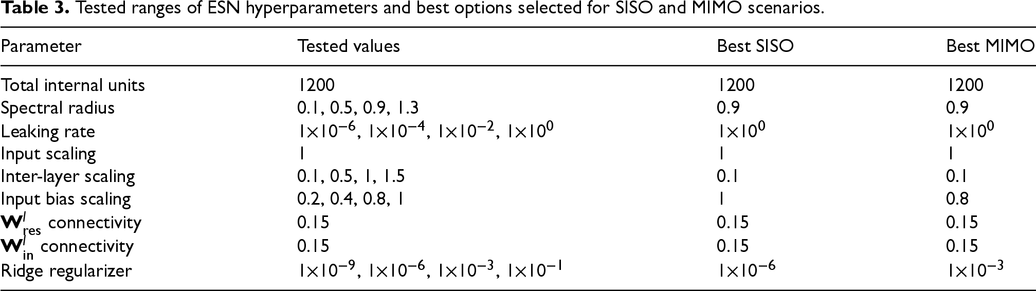
Tested ranges of ESN hyperparameters and best options selected for SISO and MIMO scenarios.
In contrast, the scaling of the first input weight matrix
The best hyperparameters for each scenario, model configuration and number of layers are chosen based on the lowest RMSE value obtained on the validation dataset. Even though there are minor variations depending on the number of layers used, the best hyperparameters are the same for almost all the tested setups within the same scenario. Those best values are also shown in Table 3.
Once the best hyperparameters for each setup are defined, new randomly initialised models are trained for each number of layers within the given range, and the performance of the models is evaluated on the test dataset. Given the randomness implicit in the ESNs, this process is repeated five times to analyse the variability of the results, calculating the mean loss and its standard deviation.
The mean test RMSE obtained and the corresponding standard deviation are presented in Figures 6 to 8, for the SISO-UP, SISO-LO and MIMO-LO scenarios, respectively. It should be noted that the 4-TANK setup is included in all the scenarios, particularised for the corresponding tank, and considering the value of the deactivated inputs as 0.
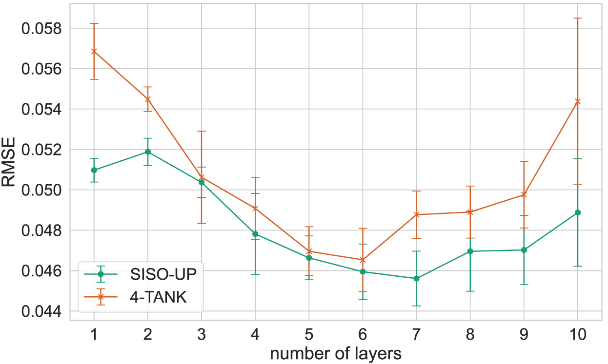
Mean RMSE and its standard deviation obtained with Deep ESN for the upper tank.
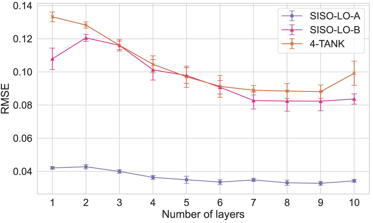
Mean RMSE and its standard deviation obtained with Deep ESN for the lower tank in SISO scenario.
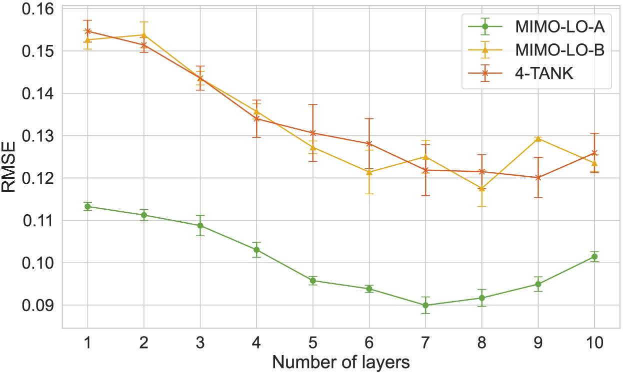
Mean RMSE and its standard deviation obtained with Deep ESN for the lower tank in MIMO scenario.
The results show that the performance of the models improves as the number of layers increases, with the RMSE decreasing and the
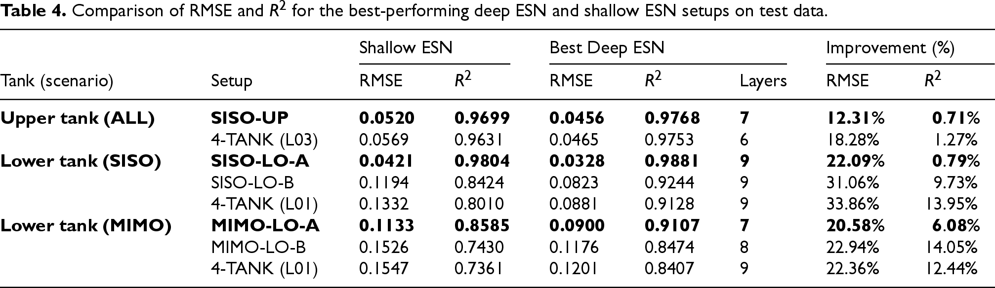
Comparison of RMSE and
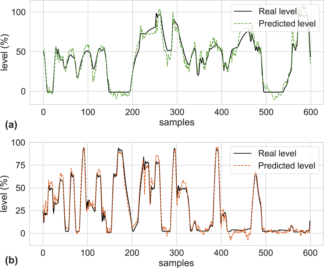
Prediction for lower and upper tanks with the selected best Deep ESN setups. (a) Prediction for the lower tank (tank 1) with the best Deep ESN MIMO-LO-A setup and (b) Prediction for the upper tank (tank 3) with the best Deep ESN SISO-UP setup.
It can be observed that the improvement in RMSE ranges from 12.31% to 33.86%, and the improvement in
In contrast, the setup for the lower tank with the best improvement is the SISO-LO-B, with a 31.06% reduction in RMSE and a 9.73% increase in
The best Deep ESN setups are selected based on the best performance metrics obtained as follows. On the one hand, for the upper tanks there are two possible setups for both SISO and MIMO scenarios, which are the SISO-UP and the 4-TANK setup. Among these setups, the best one is the SISO-UP setup with a Deep ESN of 7 layers.
On the other hand, for the lower tank there are three possible setups for the SISO scenario and three setups for the MIMO scenario. Among these setups, the best one in the SISO scenario is the SISO-LO-A setup with a Deep ESN of 9 layers; and the best in the MIMO scenario is also the MIMO-LO-A setup with a Deep ESN of 7 layers.
Taking this into account, to model the level of the lower tanks only P02 and V02 are working (SISO scenario), the SISO-LO-A setup with a Deep ESN of 9 layers can be used. However, if both pumps and valves are connected (MIMO scenario), the MIMO-LO-A setup with a Deep ESN of 7 layers should be used instead. For this reason, the MIMO-LO-A setup is selected to model the levels of the lower tanks, as it is the one that can be used in both scenarios.
Therefore, the SISO-UP and MIMO-LO-A setups are the most suitable for modelling the upper and lower tanks, respectively, and are the ones that will be used in the next steps of the implementation process. To conclude this step, Figure 9 shows the performance of the best Deep ESN setups compared to the real levels for each of the tanks.
The next step in the implementation process is to evaluate the performance of the selected Deep ESN setups against LSTM reference models. The LSTM models are trained, validated and tested with the same data as the ESN models. As two different setups were selected for Deep ESN models, one to predict the level of the upper tanks (SISO-UP) and another one to predict the level of the lower tanks (MIMO-LO-A), two LSTM models are trained for each of the setups.
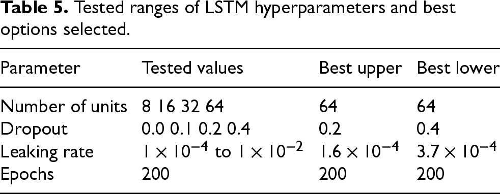
The hyperparameters of the LSTM models are selected from the ranges of values shown in Table 5, using a Tree-structured Parzen Estimator (TPE) algorithm in this case. This algorithm is chosen because it is more suitable for models with long training times and slower convergence, such as LSTM models.
Tested ranges of LSTM hyperparameters and best options selected.
Tested ranges of LSTM hyperparameters and best options selected.
The comparison between the Deep ESN and LSTM models is performed in terms of RMSE and
Performance of LSTM compared to the selected ESN and deep ESN setups.
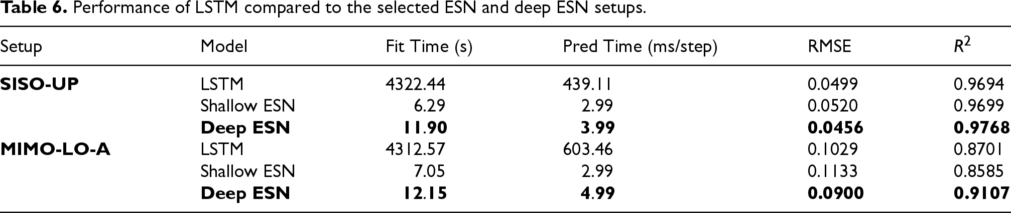
The table shows that even with similar results in terms of RMSE and
Thus, while Shallow ESNs are already able to outperform LSTM models in terms of training and prediction time, Deep ESN models not only continue to outperform in these terms, but also improve in RMSE and
Moreover, in order to obtain a performance similar to that of Deep ESN models, LSTM models need to be much larger, with many more trainable parameters than ESN models: in the performed experiments, about 17217 trainable weights are handled in LSTM models compared to 1201 in ESN models, taking into account that in ESN models only the 1200 readout weights and the output bias are trained.
While Shallow ESNs already offer a good balance between simplicity and efficiency, the results show that Deep ESNs provide additional improvements in accuracy, especially in more complex setups such as MIMO-LO-A. In these scenarios, where dynamic interactions and multi-scale temporal behaviours are more significant, the layered structure of Deep ESNs captures the underlying system dynamics more effectively. Although adding more reservoir layers slightly increases computational time, the improvement in prediction performance makes Deep ESNs particularly valuable for industrial systems that require greater modelling accuracy.
The final step in the implementation process is to deploy the selected Deep ESN models on embedded devices with limited computational resources, to evaluate the performance of the models in real-time industrial applications. In this case, both selected Deep ESN models for SISO-UP and MIMO-LO-A setups are implemented, taking into account the training time, the prediction time for the whole test dataset, and the prediction time per sample. The evaluation is performed on three different embedded devices: a Raspberry Pi Zero 2 W, a Magelis IIot Core Box from Schneider Electric, and a Simatic IoT2050 from Siemens. The results obtained are compared with the performance metrics obtained on a desktop PC, which was used for the previous training, hyperparameter search, evaluation and model selection tasks.
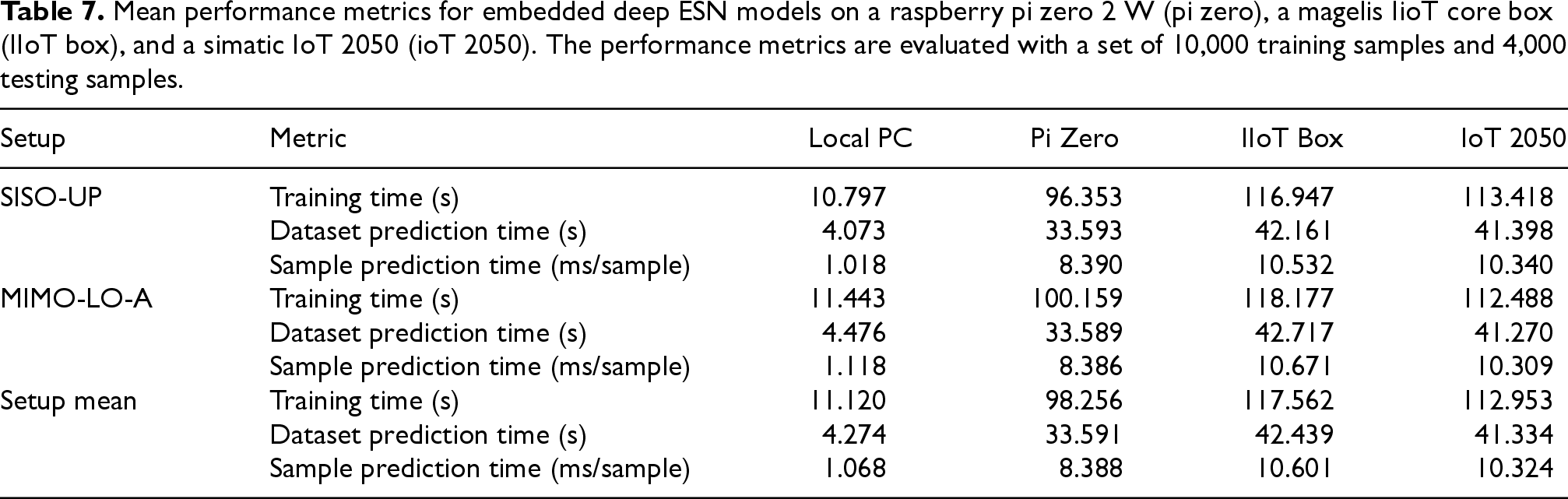
The performance metrics obtained for the selected Deep ESN models on the different devices are shown in Table 7. The table shows the mean training time, the mean prediction time for the whole test dataset, and the mean prediction time per sample for the SISO-UP and MIMO-LO-A setups.
Mean performance metrics for embedded deep ESN models on a raspberry pi zero 2 W (pi zero), a magelis IioT core box (IIoT box), and a simatic IoT 2050 (ioT 2050). The performance metrics are evaluated with a set of 10,000 training samples and 4,000 testing samples.
Mean performance metrics for embedded deep ESN models on a raspberry pi zero 2 W (pi zero), a magelis IioT core box (IIoT box), and a simatic IoT 2050 (ioT 2050). The performance metrics are evaluated with a set of 10,000 training samples and 4,000 testing samples.
It can be seen that the three embedded devices have similar training times, averaging between 98 and 118 seconds to train the full dataset. The prediction time for the whole test dataset is between 34 and 42 seconds on the embedded devices, compared to 4 seconds on the local PC. Finally, the prediction time per sample is between 8 and 10 ms per sample, compared to 1 ms on the local PC.
The results show that the mean training times are significantly higher on the embedded devices than on the local PC, with an increase of about 10 times. However, the prediction times are still acceptable for real-time applications, with an mean prediction time per sample of about 10 ms, which is suitable even for the control of industrial processes. Therefore, the results show that the selected Deep ESN models are able to function in real-time on embedded devices, with a suitable performance for industrial applications.
This work assesses the performance of Deep Reservoir Computing models when implemented in real-time industrial applications on embedded devices. The proposed approach is applied to a four-tank industrial process. The implementation process is structured in three main steps: the selection of the best Deep RC architectural setup, the comparison of the selected models with LSTM reference models, and the implementation of the selected models on embedded devices.
The results show that the Deep ESN models outperform the LSTM models in terms of training and prediction times, while also offering similar performance in terms of RMSE and
These findings highlight the potential of Deep ESNs as lightweight and efficient models well-suited to the increasing demand for real-time machine learning solutions in industrial applications. Their reduced computational cost, combined with competitive accuracy, makes them attractive for deployment in constrained embedded environments.
Finally, implementing the selected Deep ESN models on embedded devices demonstrates their ability to operate in real-time, achieving a mean prediction time per sample of approximately 10 ms. This performance makes them appropriate even for industrial process control. The results show that Deep ESN models are suitable for implementation on embedded devices, as they offer similar performance to LSTM models, but with much shorter training and prediction times.
Nonetheless, certain limitations should be noted. One challenge relates to the scalability and generalization of the models when applied to larger or more complex industrial systems. In such cases, the reservoir matrices may grow too large to be processed efficiently on embedded hardware. One possible solution is to adopt a modular approach, whereby the overall system is decomposed into smaller, semi-independent subsystems, each of which is handled by its own Deep ESN, as has been done with the four-tank system. This decomposition would simplify dynamics and allow computational resources to be distributed more effectively.
For this reason, to expand the proposed approach to broader industrial environments, future work will explore the integration of multiple Deep ESNs in a distributed architecture, with each model responsible for a subset of variables or a specific process section.
Future work will also focus on implementing Deep ESN models in a real-time control system to evaluate their performance in real industrial applications. In addition, the possibility of adapting the models in real time with online readout on embedded devices will be tested, as has been done in previous works with Shallow ESNs on desktop PCs. This would allow real-time adaptation of Deep ESN models to changes in the system, which could further improve their performance in real-time industrial applications. Analysing how energy consumption increases when more reservoir layers are added is also particularly important for deploying the models on embedded systems. Therefore, this is another key area for future research.
The robustness of the models in the presence of real industrial noise and operating variability, which are common in production environments, will also be the subject of examination in future work. In addition, neural network ablation studies may be conducted to evaluate the relative contribution of each reservoir layer and connection pattern. This analysis could provide insights for optimizing the architecture and further reducing computational load without compromising performance.
Finally, future work could also explore potential applications of Deep ESN-based models not only for control but also for real-time anomaly detection, leading to intelligent monitoring solutions in industrial systems.
Footnotes
Funding
This work was supported by the Spanish State Research Agency, MCIN/ AEI/ 10.13039/ 501100011033 under Grants PID2020-117890RB-I00 and PID2020-115401GB-I00; and by EU-EIC EMERGE (Grant No. 101070918) and NEURONE, a project funded by the Italian Ministry of University and Research (PRIN 20229JRTZA). The work of José Ramón Rodríguez-Ossorio was supported by a grant from the 2020 Edition of Research Programme of the University of León.
Declaration of conflicting interests
The author(s) declared no potential conflicts of interest with respect to the research, authorship, and/or publication of this article.