Solving the energy-aware flexible job shop problem using a memetic algorithm

Abstract

This article addresses the flexible job shop problem with interval processing times. Minimising makespan is a well-known scheduling objective that is widely used in many sectors; however, energy efficiency is gaining more importance as climate change intensifies. In this work, we minimise the makespan and the total energy consumption using a lexicographic goal programming approach. A memetic algorithm that is composed of a genetic algorithm and a local search method is developed and tested to solve this problem. The results show that our approach manages to improve the best-known results.

1. Introduction

Scheduling problems focus on distributing limited resources across multiple tasks while meeting specific constraints. ¹ Perhaps the best-known application of scheduling is in manufacturing, for instance, in weapon industry, ² automobile parts industry, ³ or steel production.^4,5 However, scheduling is also relevant in many other areas, including transportation and logistics,^6–8 electric vehicle charging, ⁹ healthcare,^10,11 education,^12,13 and cloud computing. ¹⁴ There are many examples of real-life applications of scheduling problems in the literature; for instance, Martins et al. ¹⁵ propose an algorithm to schedule analytical chemistry tests for a quality control problem of a real-world pharmaceutical company. Another example is an application of scheduling to travel-optimised warehouses in a logistic company where the authors propose a GRASP-based algorithm. ¹⁶

It is evident that the majority of these problems are intractable due to their inherent complexity. Consequently, precise algorithms cannot be implemented, with the exception of the smallest instances. In light of these challenges, researchers have been developing approximate search strategies that, while no longer guaranteed to achieve optimal results, can provide satisfactory solutions within a reasonable time frame. ¹⁷

Natural phenomena, such as evolution, ¹⁸ hydrology and hydrodynamics, ¹⁹ neurobiological systems, ²⁰ or the behaviour of materials, ²¹ have proven to be a fruitful source of inspiration to design such algorithms, often within the field of metaheuristic search. Metaheuristics have also been inspired by mimicry, such as musicians looking for pleasing harmony or animals searching food.^22–24 In parallel, the design of metaheuristic methods for hard optimisation problems has advanced considerably with the development of learning methods, sometimes enriching hybrid metaheuristics. ²⁵

Within scheduling, the job shop problem (JSP) in its multiple variants constitutes a vibrant field of research simulating practical, technical, and social applications. ²⁶ Here, tasks are organised into jobs, so tasks in the same job must be completed in a specific order on specific machines. The flexible job shop scheduling problem (FJSP) is a variant that allows some or all tasks to be executed on multiple machines.^27,28 This flexibility results in variability in processing times and energy consumption depending on the machine used.

Even the simplest forms of JSP are NP-hard, ²⁹ motivating the use of approximate metaheuristic search algorithms from the field of Artificial Intelligence as solving methods.^30,31 These methods work by exploring different possible schedules and evaluating their quality based on criteria such as makespan, energy consumption, due-date satisfaction or machine use.^27,32 In particular, memetic algorithms, which combine a metaheuristic with a local search method, are successfully applied to solve these problems. ³³ To mention but a few, in Mencía et al. ³⁴ a JSP with operators is solved using various memetic algorithms, Afşar et al. ³⁵ propose an enhanced memetic algorithm to solve a fuzzy variant of JSP, while a different memetic algorithm is used for the fuzzy FJSP. ³⁶

Traditionally, scheduling has been concerned with optimising production-related functions, most famously, to reduce the makespan, which is the time required to complete all tasks. However, due to climate change and the need for energy efficiency, there is a growing focus on optimising processes with a consideration for sustainability.^37–40 With manufacturing consuming an estimated 37% of global resources, ⁴¹ it seems essential to incorporate environmental and energy awareness into scheduling processes. In order to ensure the ongoing viability of this fundamental activity and to mitigate the effects of global warming, it is imperative that industry adopts more efficient technologies. These technologies must enable a reduction in energy consumption and emissions without compromising productivity. Consequently, there has been a consistent increase in the volume of research allocated to the domains of energy efficiency and sustainability within the realm of manufacturing engineering. ⁴² Also, according to the 2024 report of the International Energy Agency, ⁴³ global data centres are projected to double their electricity consumption by 2026, primarily driven by the growing demand for AI and digital infrastructures. Hence, as cloud computing becomes integral to modern digital infrastructure, energy-efficient scheduling gains more importance. ⁴⁴ Overall, green scheduling seems necessary to achieve the Sustainable Development Goals, in particular to “promote sustainable industrialization” (Goal 9) and “ensure sustainable consumption and production patterns” (Goal 12). ⁴⁵

In most cases, energy-related objectives must be considered in combination with more traditional production-related objectives, such as makespan or tardiness minimisation. ⁴⁶ Perhaps the most common approach in the literature is to assume that all objectives are equally important and use a Pareto approach. ³⁵ However, in many production environments objectives of different nature have different priorities and hence a hierarchical approach is more appropriate. For instance, a recent review ⁴⁷ suggests that economic objectives minimising costs and maximising profits are of primary importance to decision makers, with criteria related to minimising the environmental impact of production processes coming in second place.

Traditionally, all parameters in scheduling problems are assumed to be deterministic and well known in advance. However, in reality, many factors such as processing times can vary due to machine or human influences. Uncertainties in increasingly complex environments should be addressed to properly handle the variable nature of various elements of the scheduling process. Uncertainty management will be particularly important in Industry 5.0 solutions that will require close integration of operators and technical systems. ⁴⁸ In the literature, uncertain task durations are typically addressed with stochastic models, where these durations are represented by probability distributions. However, gathering sufficient data to estimate an accurate probability distribution is often not feasible, and, even if such an accurate distribution is available, the associated computational load can be excessive. An alternative is to use fuzzy numbers to model uncertain processing times, particularly in FJSP, which requires less detailed information and offers computational efficiency.^36,49,50 Furthermore, in those scenarios, where prior knowledge is very limited, interval-based models can be employed, using only lower and upper bounds to describe task durations. These intervals can be interpreted as uniform probability distributions in the absence of more specific information. Although simple, this modelling allows to obtain more robust solutions, with a performance that is less susceptible to slight variations in task durations. ⁵¹

Despite the fact that the interval approach is a straightforward uncertainty model, the existing body of literature in interval JSP and FJSP is limited. A genetic algorithm is proposed to reduce tardiness in a JSP with interval due dates and process durations. ⁵² A hybrid methodology integrating particle swarm optimisation and a genetic algorithm tackles a FJSP with interval processing times in a larger framework of integrated planning and scheduling problem. ⁵³ Multi-objective interval JSPs are examined in two different papers.^54,55 In the first one, an artificial bee colony algorithm is used to minimise both makespan and total tardiness in JSP with flexible maintenance and non-resumable jobs. In the latter, carbon footprint and makespan are minimised lexicographically in a dual-resource restricted JSP with heterogeneous resources using a dynamic neighbourhood search. More recently, Díaz et al. ⁵⁶ consider a JSP with interval task durations and propose a genetic method to minimise makespan. The same problem is addressed employing a variant of artificial bee colony algorithm that incorporates seasonal behaviour of honeybees for further intensification ²⁴ and with a memetic algorithm, combining artificial bee colony with local search. ⁵⁷

In this work, we tackle a multi-objective flexible job shop problem with interval processing times. A lexicographic goal programming approach is adopted to minimise makespan and total energy consumption and a memetic algorithm, composed of a genetic algorithm and a local search method, is developed to solve this problem. Hill Climbing (HC) and Tabu Search (TS) algorithms are tested on mono-objective versions of the problem along with tailored neighbourhood structures. Our contributions can be summarised as follows.

Three new neighbourhood structures are defined and tested for each objective

Two local search methods combined with a genetic algorithm have been developed and tested to solve the mono-objective problems

The approaches that give the best results for the mono-objective cases are integrated to solve the multi-objective problem with lexicographic goal programming

The experimental results show that the memetic algorithm manages to improve the best-known solutions of this problem.

We formally define the problem in the Problem Definition Section. Later, we describe our solution approach in detail in Solution Methodology and present the experimental results in the Experimental Results Section. Lastly, the conclusions of our work are given in the Conclusion Section.

2. Problem definition

In the deterministic job shop problem (JSP), a set of $n$ jobs, which can be denoted by $J$ , should be completed. Each job $j$ is composed of a set of tasks $O_j=\{o_{j1},\dots ,o_{j{N}_j}\}$ that need to be processed on a specific machine from the set of $m$ machines $M$ . Moreover, tasks in a job should be processed in a particular order, often referred to as job precedence constraints.

In the flexible variant of JSP, a task $o_{ji}$ can be processed on a machine $k$ from a set of alternatives denoted $M(o_{ji})$ . The processing time of a task $o_{ji}$ depends on the machine on which it is performed and is denoted by $d_{jik}$ . The tasks are non-pre-emptive: they cannot be interrupted until they finish, and a machine cannot work on more than one task at a time.

Processing times are not the only parameters that depend on the task and the machine in the energy-aware version of the FJSP. The amount of active power needed by a machine $k\in M(o_{ji})$ changes depending on the task $o_{ji}$ it is executing, and therefore it is denoted as $A{P}_{jik}$ . Besides the active power, each machine $k$ needs a certain amount of passive power, $P{P}_k$ , while it is on.

A feasible solution of this problem has two components: an assignment of every task to a machine $\mathit{\tau }$ and a feasible schedule $\mathit{s}$ , composed of the starting times of all tasks on the selected machines whilst complying with all the other constraints. In our study, two objectives are considered in a lexicographical manner, i.e., the primary objective is to minimise the makespan, whereas the secondary objective is to minimise the total energy consumption.

In real-world settings, the time needed to complete a task is often uncertain and not precisely known beforehand. Usually, only rough estimates of the duration are available. When only the minimum and maximum times are known for each task, this uncertainty can be represented using a closed interval, denoted $\mathbf{\text{a}}=[a^1,a^2]=\{x\in \mathbb{R}:a^1\le x\le a^2\}$ . In this work, we denote the FJSP with interval uncertainty as Interval Flexible Job Shop (IFJSP).

To calculate our objective functions on a schedule with interval processing times, we require arithmetic operations like addition and maximum between intervals, as well as the addition and multiplication between a scalar value an an interval. ⁵⁸ Assuming that $\mathbf{\text{a}}=[a^1,a^2]$ and $\mathbf{\text{b}}=[b^1,b^2]$ are two intervals, the addition is defined as $\mathbf{\text{a}}+\mathbf{\text{b}}=[a^1+b^1,a^2+b^2]$ and the maximum is calculated as $max(\mathbf{\text{a}},\mathbf{\text{b}})=[max(a^1,b^1),max(a^2,b^2)]$ . Given an interval $\mathbf{\text{a}}$ and a value $r\in \mathbb{R}$ , the addition and product are defined, respectively, as $\mathbf{\text{a}}+r=[a^1+r,a^2+r]$ and $r\mathbf{\text{a}}=[r{a}^1,r{a}^2]$ . When comparing values, closed intervals are not endowed with a natural ordering. Instead, various ranking methods are used in the literature. ⁵⁹ . In a recent interval scheduling research work, ²⁴ several ranking methods are compared in terms of robustness, supporting the extended use of the midpoint ranking (MP). This has become the most widely used comparison method, where $\mathbf{\text{a}}{\le }_{MP}\mathbf{\text{b}}$ if and only if $m(\mathbf{\text{a}})\le m(\mathbf{\text{b}})$ , with $m(\mathbf{\text{a}})=(a^1+a^2)/2$ .

2.1. The objectives

In this work, we optimise a multi-objective IJSP using lexicographic goal programming. Our primary objective is to minimise makespan, which is the earliest time by which all jobs have been completed. Denoting the starting time of the last task in job $j$ by ${\mathit{s}}_{\mathit{j}{\mathit{N}}_{\mathit{j}}}=[s_{j{N}_j}^1,s_{j{N}_j}^2]$ , we can define the makespan as ${\mathit{C}}_{\mathbf{max}}=max\{{\mathit{s}}_{\mathit{j}{\mathit{N}}_{\mathit{j}}}+{\mathit{d}}_{\mathit{j}{\mathit{N}}_{\mathit{j}}{\mathit{k}}_{{\mathit{N}}_{\mathit{j}}}}:j\in J\}$ . Since it is an interval, we use the midpoint ranking to choose the best makespan value.

Our second objective is the minimisation of energy consumption. In the literature on manufacturing systems, there are many works that propose sophisticated energy-consumption models.^60–62 However, in the energy-aware scheduling literature, simpler methods have been proposed to incorporate energy impact into schedule optimisation. For instance, González, Oddi and Rasconi ⁶³ focus solely on the energy consumed when machines are idle, whereas a more recent work assumes that all machines remain on from the beginning until the last task is completed. ³⁶ In this study, we assume that each machine $k\in M$ starts in the off state and does not consume energy until an operator switches it on. It is reasonable to assume that workers act conservatively, activating the machine only when there is a potential need for it, specifically at the earliest possible starting time of the first task assigned to it, $f_k$ , denoted as $s_{f_k}^1$ , where ${\mathit{s}}_{{\mathit{f}}_{\mathit{k}}}=[s_{f_k}^1,s_{f_k}^2]$ . The machine $k$ remains on until it is no longer needed, shutting down after the completion time of its last assigned task, $l_k$ , represented by $c_{l_k}^2=s_{l_k}^2+d_{l_k}^2$ , where ${\mathit{c}}_{{\mathit{l}}_{\mathit{k}}}={\mathit{s}}_{{\mathit{l}}_{\mathit{k}}}+{\mathit{d}}_{{\mathit{l}}_{\mathit{k}}}$ based on assignment $\mathit{\tau }$ and schedule $\mathit{s}$ . During this period, the machine consumes passive power $P{P}_k$ per unit of time. The passive energy consumption of machine $k$ is therefore given by $P{E}_k=P{P}_k(c_{l_k}^2-s_{f_k}^1)$ . When machine $k$ is active and executing a task $o_{ji}$ , it consumes power at a rate of $A{P}_{jik}$ per unit of time. The active energy consumption of $k$ is calculated as $\mathit{A}{\mathit{E}}_{\mathit{k}}=\sum _{j,i:{\tau }_{ji}=k}(A{P}_{jik}{\mathit{d}}_{\mathit{j}\mathit{i}\mathit{k}})$ , with $j\in J$ , $i\in O_j$ . Notably, active energy depends on the machine and the task duration, which remains uncertain in this problem, whereas passive energy is deterministic, based on the worker’s decision to turn machines on and off. The total energy consumption is then defined as $\mathit{T}\mathit{E}=\sum _{k\in M}(P{E}_k+\mathit{A}{\mathit{E}}_{\mathit{k}})$ . Additionally, we can consider the passive energy $P{E}_k$ as being divided in two parts: the energy consumed while potentially executing a task and the idle energy, which is consumed when the machine is idle with certainty.

3. Constraint programming model

Constraint programming (CP) is a mathematical modelling paradigm that involves defining a problem in terms of constraints that must be satisfied. Problems are typically modelled using variables along with their domains and constraints. CP solvers explore possible variable assignments and use inference techniques, such as constraint propagation, to reduce the search space and efficiently find solutions. ⁶⁴

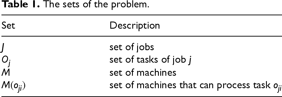
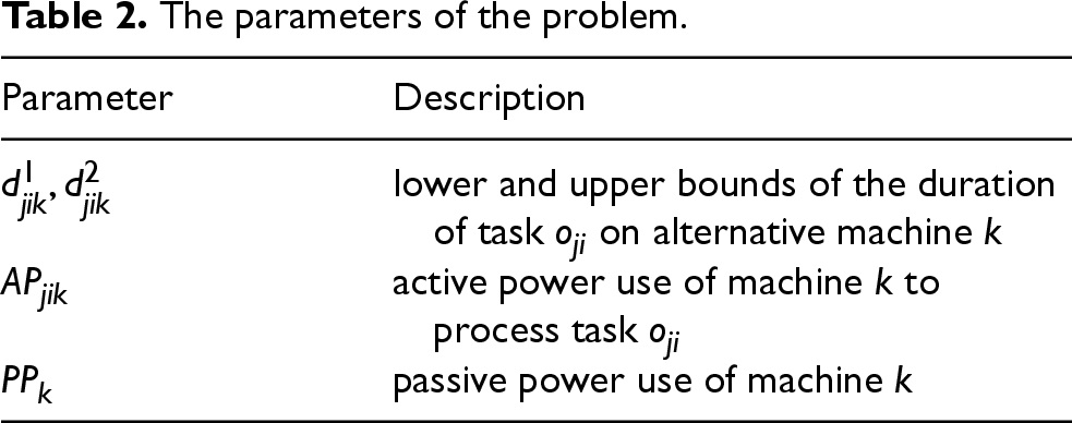
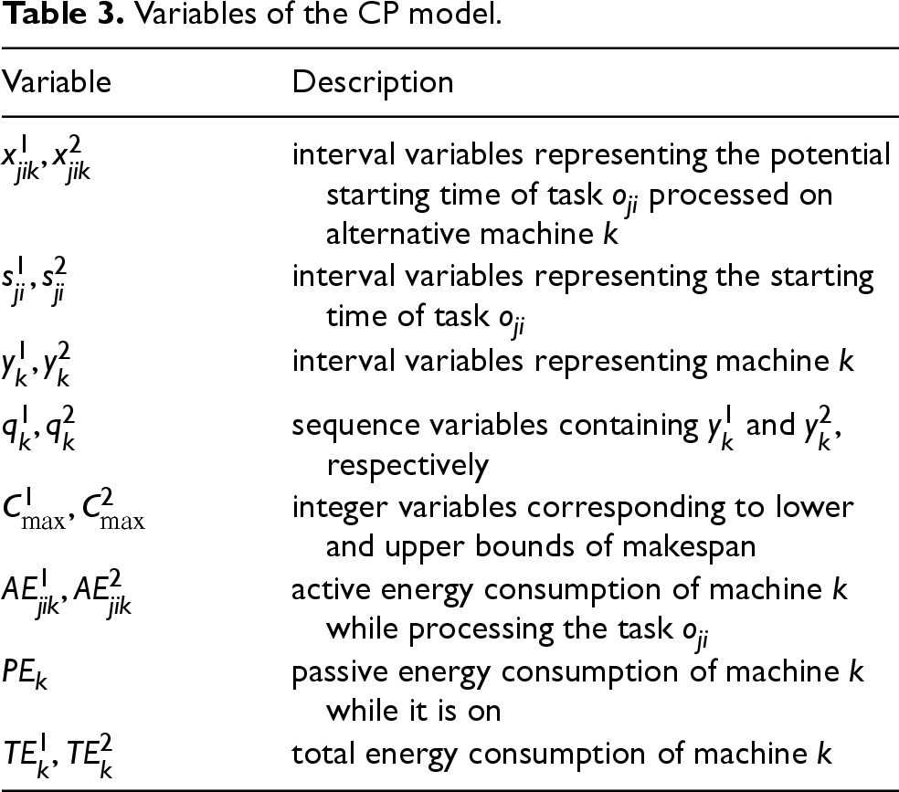
IBM ILOG CP Optimizer ⁶⁵ (CPO) is a CP solver where a task can be represented by an interval variable that has a starting point and a duration (It should not be confused with the uncertainty of processing times, which is modelled as intervals.). Since the duration of a task on machine $k$ is an interval in our problem, i.e., ${\mathit{d}}_{jik}=[d_{jik}^1,d_{jik}^2]$ , we need to model the potential starting time of every task as a pair of optional interval variables, namely $x_{jik}^1$ and $x_{jik}^2$ with the corresponding durations. In other words, if task $o_{ji}$ is processed on alternative machine $k$ , its starting time would be the interval [ $x_{jik}^1$ , $x_{jik}^2$ ] and its ending time would be [ $x_{jik}^1+d_{jik}^1$ , $x_{jik}^2+d_{jik}^2$ ]. Moreover, task $o_{ji}$ can be processed on one machine only, and hence only one pair of these optional variables would be present in a feasible solution. The actual starting time of task $o_{ji}$ in the selected machine is modelled by the interval variables $s_{ji}^l$ , $l\in \{1,2\}$ and these will have the same value as the $x_{jik}^l$ present in the solution. Another type of variable that is introduced in CP Optimizer to facilitate the modelling of a machine is sequence variable which is defined as an unordered set of interval variables. More precisely, since tasks are modelled as interval variables, a machine is modelled as a sequence of tasks ( $q_k^l$ ) whose order is decided during the resolution phase. Another pair of interval variables, namely $y_k^1,y_k^2$ , are introduced to compute the passive energy consumption of a machine $k$ , $P{E}_k$ . The sets, parameters and variables of the CP model are given in Tables 1 to 3 along with their descriptions, respectively.

Table 1.

The sets of the problem.

Set	Description
$J$	set of jobs
$O_j$	set of tasks of job $j$
$M$	set of machines
$M(o_{ji})$	set of machines that can process task $o_{ji}$

Table 2.

The parameters of the problem.

Parameter	Description
$d_{jik}^1,d_{jik}^2$	lower and upper bounds of the duration of task $o_{ji}$ on alternative machine $k$
$A{P}_{jik}$	active power use of machine $k$ to process task $o_{ji}$
$P{P}_k$	passive power use of machine $k$

Table 3.

Variables of the CP model.

Variable	Description
$x_{jik}^1,x_{jik}^2$	interval variables representing the potential starting time of task $o_{ji}$ processed on alternative machine $k$
$s_{ji}^1,s_{ji}^2$	interval variables representing the starting time of task $o_{ji}$
$y_k^1,y_k^2$	interval variables representing machine $k$
$q_k^1,q_k^2$	sequence variables containing $y_k^1$ and $y_k^2$ , respectively
$C_{max}^1,C_{max}^2$	integer variables corresponding to lower and upper bounds of makespan
$A{E}_{jik}^1,A{E}_{jik}^2$	active energy consumption of machine $k$ while processing the task $o_{ji}$
$P{E}_k$	passive energy consumption of machine $k$ while it is on
$T{E}_k^1,T{E}_k^2$	total energy consumption of machine $k$

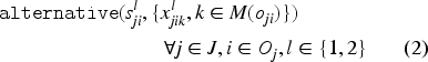
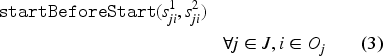
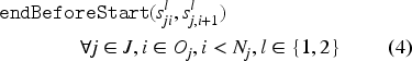
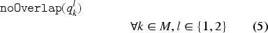
Besides interval and sequence variables, CP Optimizer also introduces several expressions that allow the user to easily define scheduling constraints. The expressions $\mathtt{s}\mathtt{t}\mathtt{a}\mathtt{r}\mathtt{t}\mathtt{O}\mathtt{f}(a)$ and $\mathtt{e}\mathtt{n}\mathtt{d}\mathtt{O}\mathtt{f}(a)$ return, respectively, the starting and ending times of an interval variable $a$ . The constraint $\mathtt{a}\mathtt{l}\mathtt{t}\mathtt{e}\mathtt{r}\mathtt{n}\mathtt{a}\mathtt{t}\mathtt{i}\mathtt{v}\mathtt{e}(a,\{b_1,\dots ,b_n\})$ ensures that, if the interval variable $a$ is present, then only one of the interval variables of the set $\{b_1,\dots ,b_n\}$ is present and it starts and ends at the same time as $a$ . The expressions $\mathtt{s}\mathtt{t}\mathtt{a}\mathtt{r}\mathtt{t}\mathtt{B}\mathtt{e}\mathtt{f}\mathtt{o}\mathtt{r}\mathtt{e}\mathtt{S}\mathtt{t}\mathtt{a}\mathtt{r}\mathtt{t}(a,b)$ (or $\mathtt{e}\mathtt{n}\mathtt{d}\mathtt{B}\mathtt{e}\mathtt{f}\mathtt{o}\mathtt{r}\mathtt{e}\mathtt{S}\mathtt{t}\mathtt{a}\mathtt{r}\mathtt{t}(a,b)$ ) guarantee that the interval $a$ starts (or ends) before the starting time of $b$ . The constraint $\mathtt{n}\mathtt{o}\mathtt{O}\mathtt{v}\mathtt{e}\mathtt{r}\mathtt{l}\mathtt{a}\mathtt{p}(c)$ prevents the intervals in a sequence $c$ from overlapping. While modelling scheduling problems using CPO, a machine is represented as a sequence of tasks, hence this constraint enforces that a machine is a unary resource. The expression $\mathtt{s}\mathtt{a}\mathtt{m}\mathtt{e}\mathtt{S}\mathtt{e}\mathtt{q}\mathtt{u}\mathtt{e}\mathtt{n}\mathtt{c}\mathtt{e}(c_1,c_2)$ obliges the sequences $c_1$ and $c_2$ to follow the same task order. The constraint $\mathtt{s}\mathtt{p}\mathtt{a}\mathtt{n}(a,\{b_1,\dots ,b_n\})$ states that the interval variable $a$ spans over $\{b_1,\dots ,b_n\}$ , that is, it starts at the same time as the first present interval in the set $\{b_1,\dots ,b_n\}$ and ends with the last one. Finally, $\mathtt{p}\mathtt{r}\mathtt{e}\mathtt{s}\mathtt{e}\mathtt{n}\mathtt{c}\mathtt{e}\mathtt{O}\mathtt{f}(a)$ is a binary expression with value 1 if the interval variable $a$ is present in the solution and 0 otherwise.

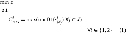
The resulting model for our problem is as follows.

$$\begin{array}{rl}{\displaystyle min}& z\\ \text{s.t.}& \\ & C_{max}^l=max(\mathtt{e}\mathtt{n}\mathtt{d}\mathtt{O}\mathtt{f}(s_{j{N}_j}^l)\mathrm{\forall }j\in J)\\ & \mathrm{\forall }l\in \{1,2\}\end{array}$$

(1)

$$\begin{array}{rl}& \mathtt{a}\mathtt{l}\mathtt{t}\mathtt{e}\mathtt{r}\mathtt{n}\mathtt{a}\mathtt{t}\mathtt{i}\mathtt{v}\mathtt{e}(s_{ji}^l,\{x_{jik}^l,k\in M(o_{ji})\})\\ & \mathrm{\forall }j\in J,i\in O_j,l\in \{1,2\}\end{array}$$

(2)

$$\begin{array}{rl}& \mathtt{s}\mathtt{t}\mathtt{a}\mathtt{r}\mathtt{t}\mathtt{B}\mathtt{e}\mathtt{f}\mathtt{o}\mathtt{r}\mathtt{e}\mathtt{S}\mathtt{t}\mathtt{a}\mathtt{r}\mathtt{t}(s_{ji}^1,s_{ji}^2)\\ & \mathrm{\forall }j\in J,i\in O_j\end{array}$$

(3)

$$\begin{array}{rl}& \mathtt{e}\mathtt{n}\mathtt{d}\mathtt{B}\mathtt{e}\mathtt{f}\mathtt{o}\mathtt{r}\mathtt{e}\mathtt{S}\mathtt{t}\mathtt{a}\mathtt{r}\mathtt{t}(s_{ji}^l,s_{j,i+1}^l)\\ & \mathrm{\forall }j\in J,i\in O_j,i<N_j,l\in \{1,2\}\end{array}$$

(4)

$$\begin{array}{rl}& \mathtt{n}\mathtt{o}\mathtt{O}\mathtt{v}\mathtt{e}\mathtt{r}\mathtt{l}\mathtt{a}\mathtt{p}(q_k^l)\\ & \mathrm{\forall }k\in M,l\in \{1,2\}\end{array}$$

(5)

$$\begin{array}{rl}& \mathtt{s}\mathtt{a}\mathtt{m}\mathtt{e}\mathtt{S}\mathtt{e}\mathtt{q}\mathtt{u}\mathtt{e}\mathtt{n}\mathtt{c}\mathtt{e}(q_k^1,q_k^2)\\ & \mathrm{\forall }k\in M\end{array}$$

(6)

$$\begin{array}{rl}& \mathtt{s}\mathtt{p}\mathtt{a}\mathtt{n}(y_k^l,\{x_{jik}^l,k\in M(o_{ji})\}))\\ & \mathrm{\forall }k\in M,l\in \{1,2\}\end{array}$$

(7)

$$\begin{array}{rl}& P{E}_k=P{P}_k*(\mathtt{e}\mathtt{n}\mathtt{d}\mathtt{O}\mathtt{f}(y_k^2)-\mathtt{s}\mathtt{t}\mathtt{a}\mathtt{r}\mathtt{t}\mathtt{O}\mathtt{f}(y_k^1))\\ & \mathrm{\forall }k\in M\end{array}$$

(8)

$$\begin{array}{rl}& A{E}_k^l=\sum _{j\in J,i\in O_j}A{P}_{jik}*d_{jik}^l*\mathtt{p}\mathtt{r}\mathtt{e}\mathtt{s}\mathtt{e}\mathtt{n}\mathtt{c}\mathtt{e}\mathtt{O}\mathtt{f}(x_{jik}^l)\\ & \mathrm{\forall }k\in M,l\in \{1,2\}\end{array}$$

(9)

$$\begin{array}{rl}& T{E}^l=\sum _{k\in M}P{E}_k+A{E}_k^l\\ & \mathrm{\forall }l\in \{1,2\}\end{array}$$

(10)

The objective function $z$ can be equal to $m({\mathit{C}}_{\mathbf{max}})$ or $m(\mathit{T}\mathit{E})$ depending on the problem to be solved. Note that in the Experimental Results Section constraints (1)-(10) have been applied to minimise the makespan ( $m({\mathit{C}}_{\mathbf{max}})$ ) and to minimise the total energy ( $m(\mathit{T}\mathit{E})$ ) individually. These mono-objective models are referred to as $C{P}_{ms}$ and $C{P}_{en}$ , respectively.

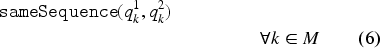
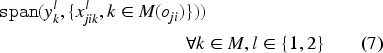
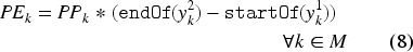
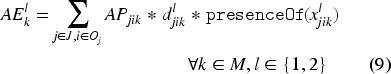
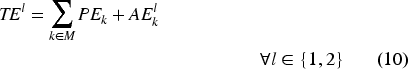
Equation (1) defines the makespan, which is calculated as the maximum of the completion times of all tasks per component $l$ . Constraint (2) makes sure that only one of the alternative intervals among all $\{x_{jik}^l,k\in M(o_{ji})\}$ is selected (or present) and starts and ends with $s_{ji}^l$ . In other words, it guarantees that a task is processed on one of the alternative machines. Constraint (3) establishes the order between the components of ${\mathit{s}}_{\mathit{j}\mathit{i}}$ to ensure the order between the lower and upper bound of the starting times. Constraint (4) sets the task precedence order in each job. Constraint (5) ensures that there is no overlap between the tasks that are processed on the same machine. Constraint (6) forces a unique processing order for the sequence variables $q_k^1$ and $q_k^2$ . Due to constraint (7), the interval variable $y_k^l$ starts with the first task that is processed on machine $k$ and ends at the same time as the last task finishes on machine $k$ . More precisely, the interval variable $y_k^l$ spans the machine $k$ and facilitates the computation of its passive energy consumption. Equation (8) computes the passive energy consumption of a machine $k$ . Equation (9) calculates the active energy consumed by machine $k$ with the help of $\mathtt{p}\mathtt{r}\mathtt{e}\mathtt{s}\mathtt{e}\mathtt{n}\mathtt{c}\mathtt{e}\mathtt{O}\mathtt{f}$ expression, which takes the value 1 if machine $k$ is selected to process task $o_{ji}$ and zero otherwise. Finally, equation (10) computes the total energy consumed by all machines processing all tasks.

4. Solution methodology

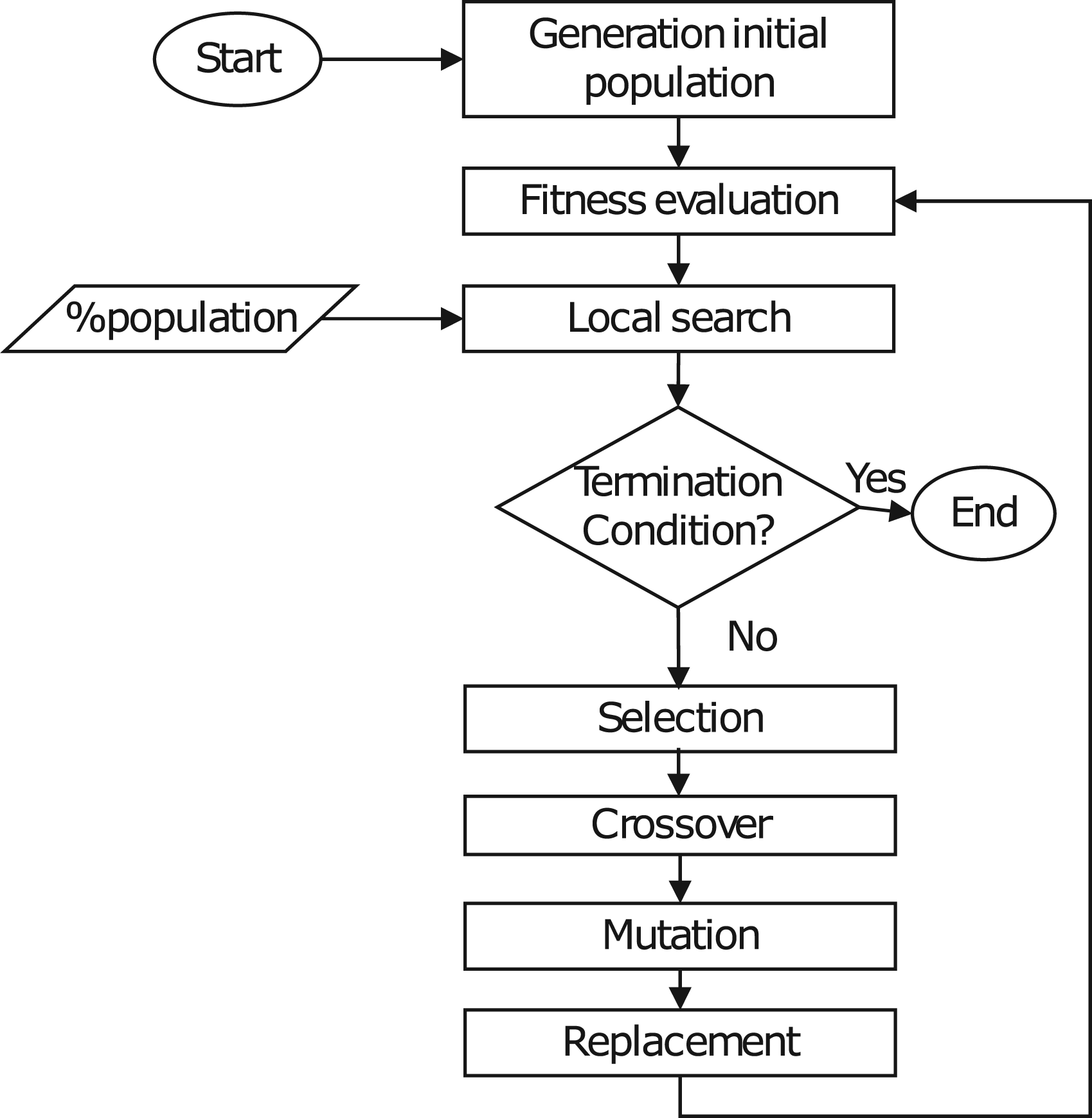
In this study, we adopt the approach proposed by Afşar et al., ⁶⁶ whereby a genetic algorithm (GA) is applied to both single and multi-objective versions of the problem. In order to improve the results, in this work we incorporate a local search strategy that is dependent on the fitness values of the solutions, resulting in a memetic algorithm (MA), whose general schema is shown in Figure 1.

Figure 1.

Diagram of the Memetic Algorithm.

4.1. Memetic algorithm

In essence, a typical local search schema begins with a given solution, proceeds to find a neighbourhood by performing some small changes, and then evaluates the neighbours in pursuit of an improved solution. Two well-known search strategies in this regard are hill-climbing and tabu search. In the proposed memetic approach, derived from the GA, we introduce a new local search stage subsequent to the fitness evaluation process. At each iteration, the local search is applied to a percentage of individuals in the current population. Furthermore, Lamarckian evolution is utilised by rebuilding the chromosome from the improved schedule obtained, thereby enabling the transfer of its characteristics to subsequent offspring.

As a novelty, the algorithm may use different local search strategies depending on the fitness of the current solution. Given the nature of our problem, if the solution subject to local search has not reached its makespan goal yet, a local search specific for this objective function is used. Otherwise, a strategy oriented towards energy consumption minimisation is employed. To do that, we introduce different neighbourhood structures depending on the objective to be optimised, ${\mathbf{C}}_{\mathbf{m}\mathbf{a}\mathbf{x}}$ or $\mathbf{T}\mathbf{E}$ .

4.2. Neighbourhood structures

In the context of optimising ${\mathbf{C}}_{\mathbf{m}\mathbf{a}\mathbf{x}}$ , three distinct neighbourhood structures are employed. The first one, designated $N^{Mct}$ , is based on the neighbourhood structure introduced by González Rodríguez et al. ⁶⁷ There, the authors propose the use of parallel graphs to extend the concepts of critical paths and critical blocks used by Van Laarhoven, Aarts and Lenstra ⁶⁸ to fuzzy job shop scheduling. The same principle can be used in our problem, representing a solution as two parallel graphs and defining a critical task as one that belongs to the critical path of any of the parallel graphs. Specifically, a neighbour is created by reversing a critical arc that is at the beginning or end of a critical block. For the second neighbourhood, designated $N^{Mmac}$ , each neighbour is generated by taking a critical task $o_{ji}$ and reassigning it to any of its available machines $M(o_{ji})$ . Following Palacios et al., ⁴⁹ the task is assigned to its new machine at the earliest possible starting time that maintains the prior relative task order. The final neighbourhood, designated $N^{Mall}$ , is formed as a superset resulting from the merging of the two earlier ones, $N^{Mall}=N^{Mct}\cup N^{Mmac}$ .

To optimise $\mathbf{T}\mathbf{E}$ , we also propose three specific neighbourhoods. The initial neighbourhood, denoted $N^{Eall}$ , consists in taking a task $o_{ji}$ currently assigned to a machine $k\in M(o_{ji})$ , and reassigning it to any of its available machines $k^{\prime }\in M(o_{ji}),k\ne k^{\prime }$ where it consumes less active energy, that is, $A{P}_{ji{k}^{\prime }}{\mathbf{d}}_{\mathbf{j}\mathbf{i}{\mathbf{k}}^{\prime }}<A{P}_{jik}{\mathbf{d}}_{\mathbf{j}\mathbf{i}\mathbf{k}}$ . As in $N^{Mmac}$ , the relative order of the tasks is preserved. The computational cost of exploring this solution subspace may be considerable, depending on the amount of flexibility of the instance being solved. For this reason, the following two neighbourhoods are subsets of the former. The second neighbourhood, named $N^{Ect}\subseteq N^{Eall}$ , considers only the reassignment of critical tasks. Finally, the third neighbourhood $N^{Emin}\subseteq N^{Eall}$ considers all tasks $o_{ji}$ , but reassigns them only to the machine $k^{*}\in M(o_{ji})$ where they have minimum active energy consumption: $\mathrm{\forall }{k}^{\prime }\in M(o_{ji})A{P}_{ji{k}^{*}}{\mathbf{d}}_{\mathbf{j}\mathbf{i}{\mathbf{k}}^{\mathbf{\ast }}}\le A{P}_{ji{k}^{\prime }}{\mathbf{d}}_{\mathbf{j}\mathbf{i}{\mathbf{k}}^{\prime }}$ .

The proposed algorithm employs local search with either makespan-oriented or energy-oriented neighbourhoods, depending on the objective values of the current solution. If the solution has reached the makespan goal, neighbours are created using one of the energy-oriented neighbourhoods: $N^{Eall}$ , $N^{Ect}$ or $N^{Emin}$ . Otherwise, a makespan-oriented neighbourhood is used: $N^{Mct}$ , $N^{Mmac}$ or $N^{Mall}$ . With this setting, the algorithm does not use a neighbourhood spanning both neighbours for makespan and neighbours for energy. However, it may happen that during the same local search process, both neighbourhood types are used sequentially. That is, if local search is applied to a solution that has not reached the makespan goal, it will use a makespan-oriented neighbourhood as mentioned before, but if a solution meeting the goal is found during the local search, an energy-oriented neighbourhood will be used from that point on. To avoid losing the makespan goal, energy-oriented neighbourhoods are pruned so they do not contain solutions that can worsen ${\mathbf{C}}_{\mathbf{m}\mathbf{a}\mathbf{x}}$ .

4.3. Neighbour estimations

When using Hill Climbing, the first-evaluated neighbour that is better than the current solution is accepted as a new solution. But with Tabu Search, all the non-tabu neighbours must be explored, so the best one is accepted. Given the potential size of some of the described neighbourhoods, this can be very time-consuming, since evaluating a new solution tends to have a significant computational cost. In these cases, the use of approximate fitness functions with lower computational cost can make the local search more efficient. Let $f_{obj}(S)$ be the objective value of a solution to a minimisation problem and $f_{obj}^{\prime }(S)$ be its estimation. If the estimation is always a lower bound of the actual objective value, $\mathrm{\forall }S{f}_{obj}^{\prime }(S)\le f_{obj}(S)$ , the number of full evaluations required can be drastically decreased without loss of quality. In the Hill Climbing case, any neighbour $N(S)$ of solution $S$ such that $f_{obj}^{\prime }(N(S))>f_{obj}(S)$ can be immediately discarded knowing that $f_{obj}(N(S))>f_{obj}(S)$ as well. In Tabu Search, neighbours can be sorted according to their estimated objective value. Then, they are explored sequentially until a neighbour is found with a $f_{obj}^{\prime }$ value greater than the best $f_{obj}$ so far. At that point, there is no need to keep evaluating since the best neighbour has already been found.

For ${\mathbf{C}}_{\mathbf{m}\mathbf{a}\mathbf{x}}$ , estimations can be obtained following Palacios et al.. In that work, estimations are calculated both when a critical arc is reversed (i.e. $N^{Mct}$ ) and when a task is assigned to a different machine (i.e. $N^{Mmac}$ ). They are based on the concepts of heads and tails adapted to the case of parallel graph representation. They are also proven to be lower bounds for the actual ${\mathbf{C}}_{\mathbf{m}\mathbf{a}\mathbf{x}}$ value. In our case, we adapt the same ideas to the interval case by representing a solution with two parallel graphs instead of three. This also allows us to estimate ${\mathbf{C}}_{\mathbf{m}\mathbf{a}\mathbf{x}}$ for neighbours in the energy-oriented neighbourhoods, since they are also based on reassigning tasks to different machines.

For $\mathbf{T}\mathbf{E}$ , all the proposed neighbourhoods for this objective function involve reassigning a task to a different machine. Makespan-oriented neighbourhoods are used only when the current solution does not meet the makespan goal and energy consumption is not yet considered, so there is no need for an estimate for $\mathbf{T}\mathbf{E}$ in this case. Let $\mathit{T}\mathit{E}=\sum _{k\in M}(P{E}_k+\mathit{A}{\mathit{E}}_{\mathit{k}})$ be the objective value for the current solution and $\mathit{T}{\mathit{E}}^{\mathbf{\prime }}=\sum _{k\in M}(P{E}_k^{\prime }+\mathit{A}{\mathit{E}}_{\mathit{k}}^{\mathbf{\prime }})$ the estimation after reassigning a task $o_{ji}$ from machine $k\in M(o_{ji})$ to $k^{\prime }\in M(o_{ji})$ .

We compute $\mathit{A}{\mathit{E}}_{\mathit{k}}^{\mathbf{\prime }}$ as the sum of active energy consumed by all tasks scheduled in machine $k$ except $o_{ji}$ , $\mathit{A}{\mathit{E}}_{{\mathit{k}}^{\mathbf{\prime }}}^{\mathbf{\prime }}=A{E}_{k^{\prime }}+A{P}_{ji{k}^{\prime }}{\mathbf{d}}_{\mathbf{j}\mathbf{i}{\mathbf{k}}^{\prime }}$ , and take $\mathbf{A}{\mathbf{E}}_{{\mathbf{k}}^{″}}^{\prime }=\mathbf{A}{\mathbf{E}}_{{\mathbf{k}}^{″}}$ for any other machine $k^{″}\ne k,k^{\prime }$ . In general, $\mathrm{\forall }{k}^{″}\in M(o_{ji})P{E}_{k^{″}}^{\prime }=P{E}_{k^{″}}$ . However, if $o_{ji}$ is the first task scheduled in machine $k$ ( $o_{ji}=f_k$ ), then $P{E}_k^{\prime }=P{P}_k(c_{l_k}^2-s_{f_k^{\prime }}^1)$ , where $f_k^{\prime }$ is the successor of $o_{ji}$ in machine $k$ before reallocating. Similarly, if $o_{ji}=l_k$ , $P{E}_k^{\prime }=P{P}_k(c_{l_k^{\prime }}^2-s_{f_k}^1)$ where $l_k^{\prime }$ is the predecessor of $o_{ji}$ in machine $k$ before reallocating. If $o_{ji}=f_k=l_k$ , $P{E}_k^{\prime }=0$ . Let ${\mathbf{s}}_{\mathbf{j}\mathbf{i}}^{\prime }$ and ${\mathbf{c}}_{\mathbf{j}\mathbf{i}}^{\prime }$ be, respectively, the starting and completion times of $o_{ji}$ in machine $k^{\prime }$ after the reallocation. In that case, if ${\mathbf{s}}_{\mathbf{j}\mathbf{i}}^{\prime }<{\mathbf{s}}_{{\mathbf{f}}_{{\mathbf{k}}^{\prime }}}$ , then $P{E}_{k^{\prime }}^{\prime }=P{P}_{k^{\prime }}(c_{l_{k^{\prime }}}^2-(s_{ji}^{\prime }{)}^1)$ , and if ${\mathbf{c}}_{\mathbf{j}\mathbf{i}}^{\prime }>{\mathbf{c}}_{{\mathbf{l}}_{{\mathbf{k}}^{\prime }}}$ , then $P{E}_{k^{\prime }}^{\prime }=P{P}_{k^{\prime }}((c_{ji}^{\prime }{)}^2-s_{f_{k^{\prime }}}^1)$ .

5. Experimental results

The experimental study will be conducted in two phases. The initial series of experiments is designed to identify the most effective local search strategy and neighbourhood structures to optimise the makespan, ${\mathbf{C}}_{\mathbf{m}\mathbf{a}\mathbf{x}}$ , and the total energy consumption, $\mathbf{T}\mathbf{E}$ . In the second set of experiments, we incorporate the best-found local search strategy and evaluate the efficiency of our lexicographical proposal. Finally, we compare our method with the best one in the literature, which is, to our knowledge, the Genetic Algorithm (GA) by Afşar et al. ⁶⁶

5.1. The instance set

As a test bed, we use 12 existing instances for energy-aware IFJSP, ⁶⁶ which are based on the instances for the flexible job shop with fuzzy durations and energy costs. ⁶⁹ The latter are, in turn, adaptations of the well-known instances presented in Dauzère-Pérès and Paulli. ⁷⁰ In the fuzzy instances, the authors employ triangular fuzzy numbers to model uncertainty in task durations. In the work by Afşar et al., ⁶⁶ the middle component was discarded, and the remaining two were taken as minimum and maximum values of the interval task duration. The instances designated by $\{07a,\dots ,12a\}$ have 15 jobs and 8 resources, whereas the instances designated by $\{13a,\dots ,18a\}$ are larger, having 20 jobs and 15 resources. In addition to size, instances are classified according to the average number of machines where each task can be executed, denoted $\mu$ . Instances are divided into three categories: low flexibility instances ( $l$ ) represented by $\{$ 07a, 10a, 13a, 16a $\}$ ( $\mu \le 1.3$ ), medium flexibility instances ( $m$ ) represented by $\{$ 08a, 11a, 14a, 17a $\}$ ( $2.4\le \mu \le 3$ ) and high flexibility instances ( $h$ ) represented by $\{$ 09a, 12a, 15a, 18a $\}$ ( $\mu \ge 4.0$ ). For the sake of clarity, we include the flexibility category as a suffix of the instance names (e.g. 08a-m).

5.2. Parameter selection

For fairer comparisons, the parameters employed in this experimental study are those previously used for the GA ⁶⁶ : population size of 100 and 10,000 generations as stopping criterion. The local search is applied to 10% of the population in each generation. Each algorithm is run ten times to obtain representative values. All results have been obtained on a Linux machine equipped with two Intel Xeon Gold 6240 processors and 128GB of RAM. Detailed results are available at http://di002.edv.uniovi.es/iscop.

5.3. Lower and upper bounds

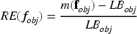
In order to facilitate more equitable comparisons, we employ the concept of relative error (RE) between the midpoint of each objective value, designated as $m({\mathbf{f}}_{obj}),obj\in \{{\mathbf{C}}_{max},\mathbf{T}\mathbf{E}\}$ and its best-known lower bound, denoted as $L{B}_{obj}$ . Given a solution, for each objective value:

$$RE(f_{obj})=\frac{m({\mathbf{f}}_{obj})-L{B}_{obj}}{L{B}_{obj}}$$

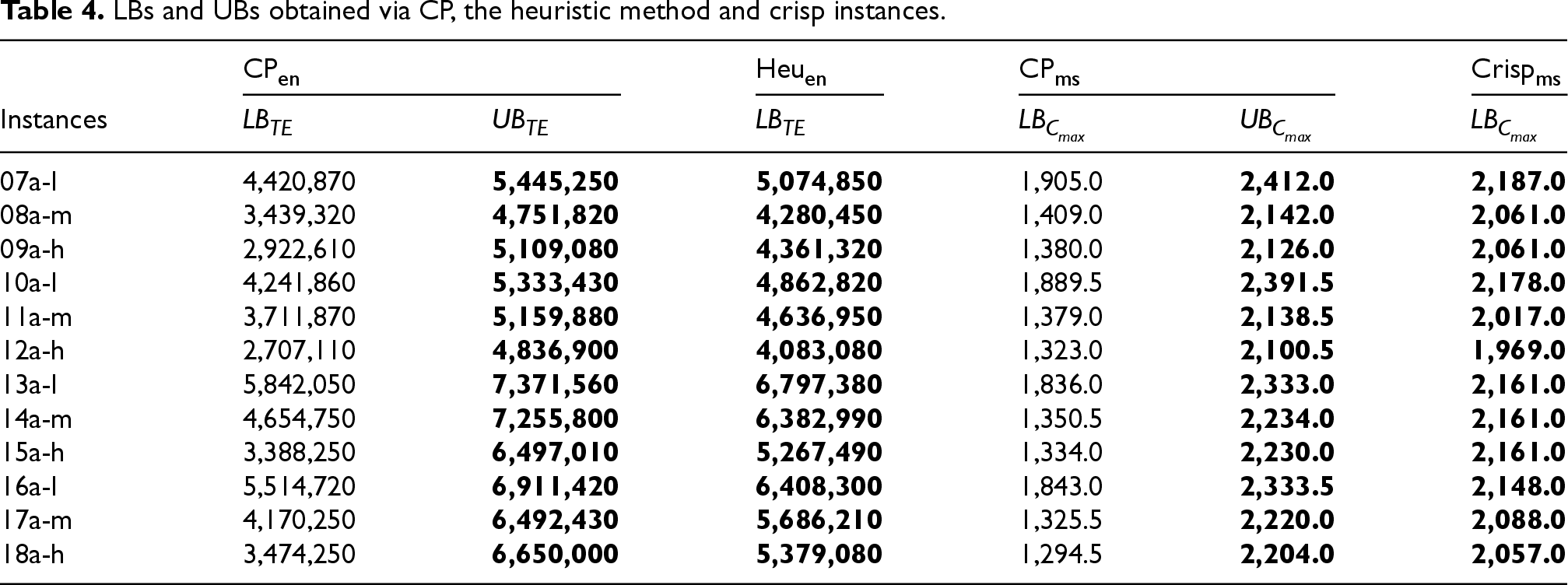
Different methods can be used to find tight lower bounds as reference point. ⁶⁶ First, the CP model described in the Problem Definition Section is solved minimising either ${\mathbf{C}}_{\mathbf{m}\mathbf{a}\mathbf{x}}$ or $\mathbf{T}\mathbf{E}$ . These are designated $C{P}_{ms}$ and $C{P}_{en}$ in Table 4 and are solved with the commercial solver IBM ILOG CP Optimizer 12.9 using an implementation in C++ with a time limit of 6 hours and a single thread. ⁶⁵ The time limit was reached in all instances, resulting in the generation of a lower and an upper bound. The mean discrepancy between the lower bound ( $LB$ ) and the optimal solution ( $UB$ ) identified by the solver after six hours is approximately 32.5% for both objectives, suggesting that the instances are not easy to solve.

Table 4.

LBs and UBs obtained via CP, the heuristic method and crisp instances.

	CP ${}_{\mathrm{en}}$		Heu ${}_{\mathrm{en}}$	CP ${}_{\mathrm{ms}}$		Crisp ${}_{\mathrm{ms}}$
Instances	$L{B}_{TE}$	$U{B}_{TE}$	$L{B}_{TE}$	$L{B}_{C_{max}}$	$U{B}_{C_{max}}$	$L{B}_{C_{max}}$
07a-l	4,420,870	5,445,250	5,074,850	1,905.0	2,412.0	2,187.0
08a-m	3,439,320	4,751,820	4,280,450	1,409.0	2,142.0	2,061.0
09a-h	2,922,610	5,109,080	4,361,320	1,380.0	2,126.0	2,061.0
10a-l	4,241,860	5,333,430	4,862,820	1,889.5	2,391.5	2,178.0
11a-m	3,711,870	5,159,880	4,636,950	1,379.0	2,138.5	2,017.0
12a-h	2,707,110	4,836,900	4,083,080	1,323.0	2,100.5	1,969.0
13a-l	5,842,050	7,371,560	6,797,380	1,836.0	2,333.0	2,161.0
14a-m	4,654,750	7,255,800	6,382,990	1,350.5	2,234.0	2,161.0
15a-h	3,388,250	6,497,010	5,267,490	1,334.0	2,230.0	2,161.0
16a-l	5,514,720	6,911,420	6,408,300	1,843.0	2,333.5	2,148.0
17a-m	4,170,250	6,492,430	5,686,210	1,325.5	2,220.0	2,088.0
18a-h	3,474,250	6,650,000	5,379,080	1,294.5	2,204.0	2,057.0

Subsequently, a heuristic method is devised which postulates that all tasks are processed on the most energy-efficient machines (i.e., those with the lowest active energy consumption for the task) among the alternatives, without pause between tasks in the same machine. The results are presented in column 4 of Table 4. This heuristic provides lower bounds for total energy consumption ( $L{B}_{TE}$ ) that are, on average, 33% more precise than those obtained by CP, despite the absence of precedence constraints.

Finally, the most widely recognised LBs for the deterministic version of FJSP that minimises makespan are considered and provided in the final column of Table 4. ⁷¹ This is due to the fact that the LBs for the crisp version of the instances are also valid $L{B}_{C_{max}}$ values. Table 4 presents a summary of all bounds for makespan and total energy. The best lower and upper bounds (LBs and UBs) are highlighted in bold and are the ones used in this work.

In our case, the makespan objective function is of primary importance and, as evidenced in Table 4, the $Cris{p}_{\mathrm{ms}}$ approach yields the best lower bounds for this objective.

5.4. Goal values

To test our proposal, we set the makespan target as $Goal=(1+\alpha )U{B}_{C_{max}}$ , where $0<\alpha <0.20$ , for each of the instances introduced before. Theoretically, given the lexicographic nature of the problem, the goal for ${\mathbf{C}}_{\mathbf{m}\mathbf{a}\mathbf{x}}$ is easier to reach when $\alpha$ is large, allowing greater focus on minimising $\mathbf{T}\mathbf{E}$ . Conversely, when $\alpha$ is small, this focus shifts towards minimising ${\mathbf{C}}_{\mathbf{m}\mathbf{a}\mathbf{x}}$ . In this study, five distinct values of $\alpha$ are employed: 0.01, 0.05, 0.10, 0.15 and 0.20; larger values of $\alpha$ have been shown to be of no special interest. ⁶⁶

5.5. Local search parameter selection

The proposed algorithm employs local search with either makespan-oriented or energy-oriented neighbourhoods, depending on the objective values of the current solution as explained in the Memetic algorithm Subsection. In that regard, to find the best neighbourhood and search strategy in each situation, we configure the local search in a single-objective version of the algorithm.

5.5.1. Search strategy

Firstly, we run a set of experiments to find the best local search strategy. We compare a Hill Climbing (HC) approach with a Tabu Search (TS) strategy. For the latter, the stopping criterion is set to 50 consecutive iterations without improvement, and the size of the tabu list is set to 18. We embed both strategies in a single-objective version of the memetic algorithm: $M{A}^{HC}$ or $M{A}^{TS}$ depending on the strategy. For the sake of clarity, the memetic algorithm minimising ${\mathbf{C}}_{max}$ is denoted as $M{A}_{ms}$ and the version minimising $\mathbf{T}\mathbf{E}$ as $M{A}_{en}$ . For his study, we use the most general neighbourhood structure in each case: $N_{ms}^{Mall}$ in $M{A}_{ms}$ and $N_{en}^{Eall}$ in $M{A}_{en}$ . We also test the algorithm without any local search and refer to it as $G{A}_{ms}$ and $G{A}_{en}$ following the same notation as MA. Finally, we shall include in our study the best upper bounds found by solving the CP model as a reference point (see Table 4).

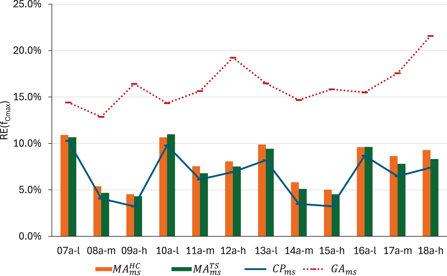
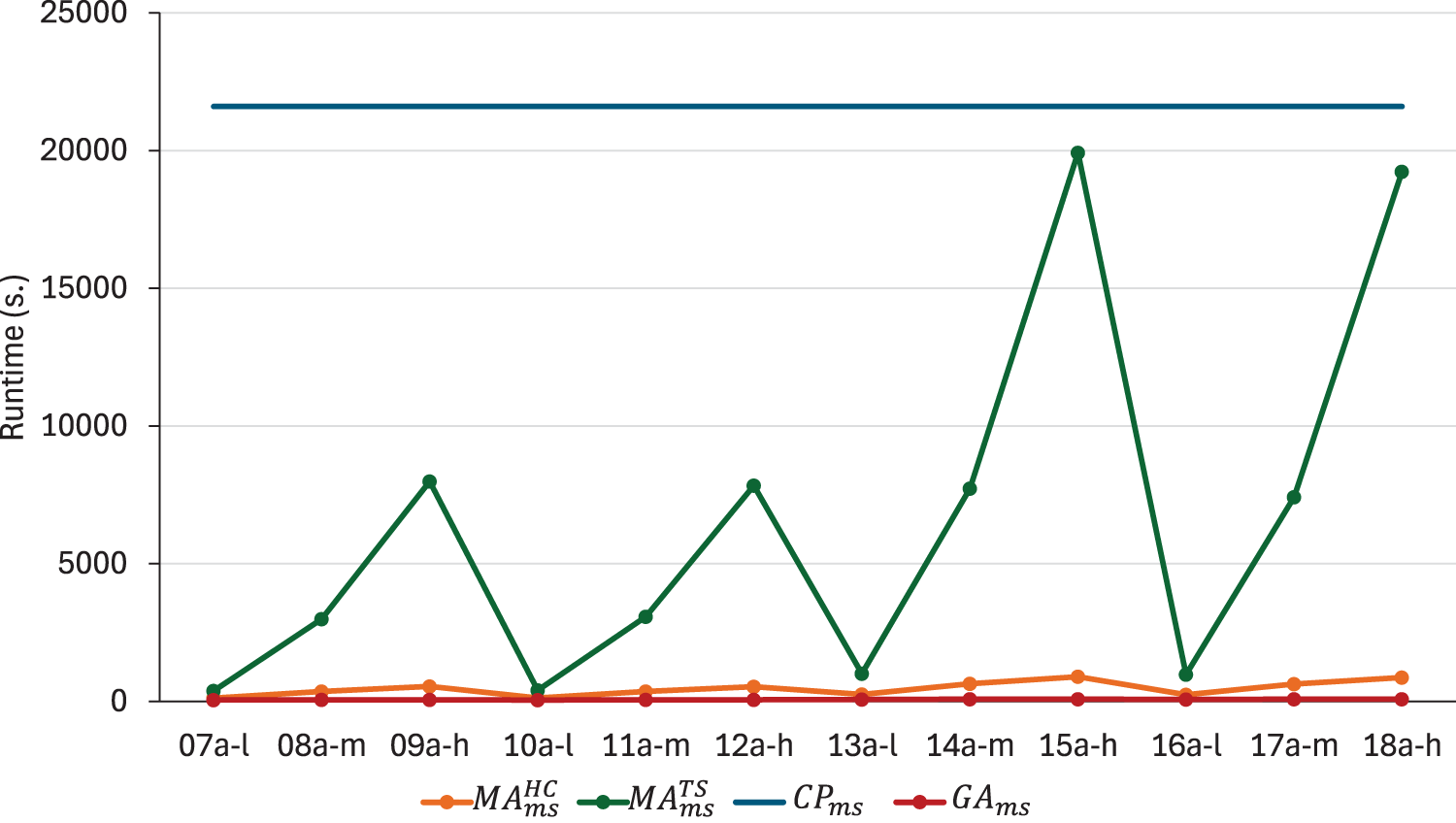
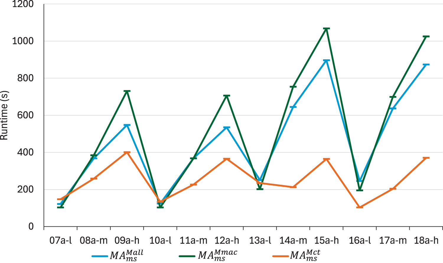
Figure 2 depicts the comparative analysis between the $RE(f_{C_{max}})$ values obtained by $M{A}_{ms}^{HC}$ and $M{A}_{ms}^{TS}$ . The $RE(f_{C_{max}})$ values obtained by $G{A}_{ms}$ and by solving $C{P}_{ms}$ are illustrated with lines. It is evident that both versions of the memetic algorithm significantly reduce the $RE(f_{C_{max}})$ values yielded by $G{A}_{ms}$ . In medium and high flexibility instances, this reduction is always above 50%, reaching up to 72,4% in instance 09a-h. Furthermore, the relative errors of the memetic solutions are comparable to the upper bounds obtained by solving the $C{P}_{ms}$ model during 6 hours. Comparing both local search strategies, there is no clear winner. $M{A}_{ms}^{TS}$ seems to be better in most instances, but not all of them, and the differences are not sufficient to justify a preference for one over the other. In this scenario, CPU times can be an indicator for decision-making. The average runtimes for all methods are shown in Figure 3. $M{A}_{ms}^{TS}$ does not seem to be a viable option in terms of computational resource consumption. The CPU time increases with both size and flexibility, with instances 15a-h and 18a-h requiring approximately 5 hours, compared to approximately 14 minutes for $M{A}_{ms}^{HC}$ . Taking into account the small differences in terms of relative errors, we consider that $M{A}_{ms}^{HC}$ represents the most reasonable choice.

Figure 2.

$RE(f_{C_{max}})$ values obtained by $M{A}_{ms}^{HC}$ , $M{A}_{ms}^{TS}$ , $C{P}_{ms}$ and $G{A}_{ms}$ .

Figure 3.

CPU time in seconds used by $M{A}_{ms}^{HC}$ , $M{A}_{ms}^{TS}$ , $C{P}_{ms}$ and $G{A}_{ms}$ .

Figure 4.

$RE(f_{TE})$ values obtained by $M{A}_{en}^{HC}$ , $M{A}_{en}^{TS}$ , $C{P}_{en}$ and $G{A}_{en}$ .

Figure 5.

CPU time in seconds used by $M{A}_{en}^{HC}$ , $M{A}_{en}^{TS}$ , $C{P}_{en}$ and $G{A}_{en}$ .

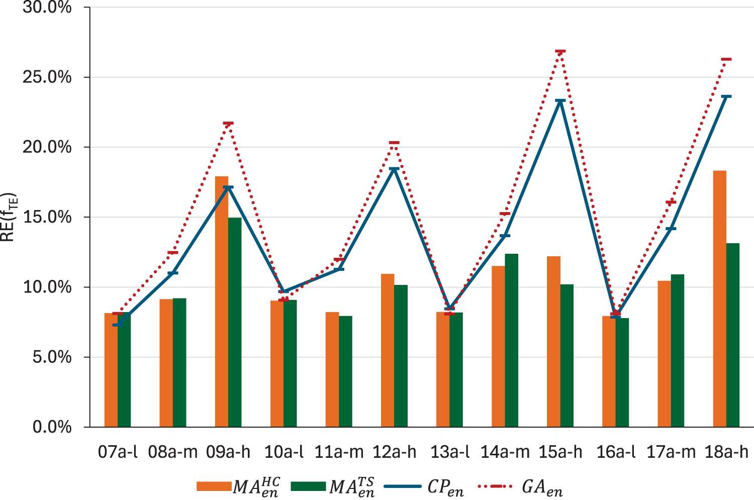
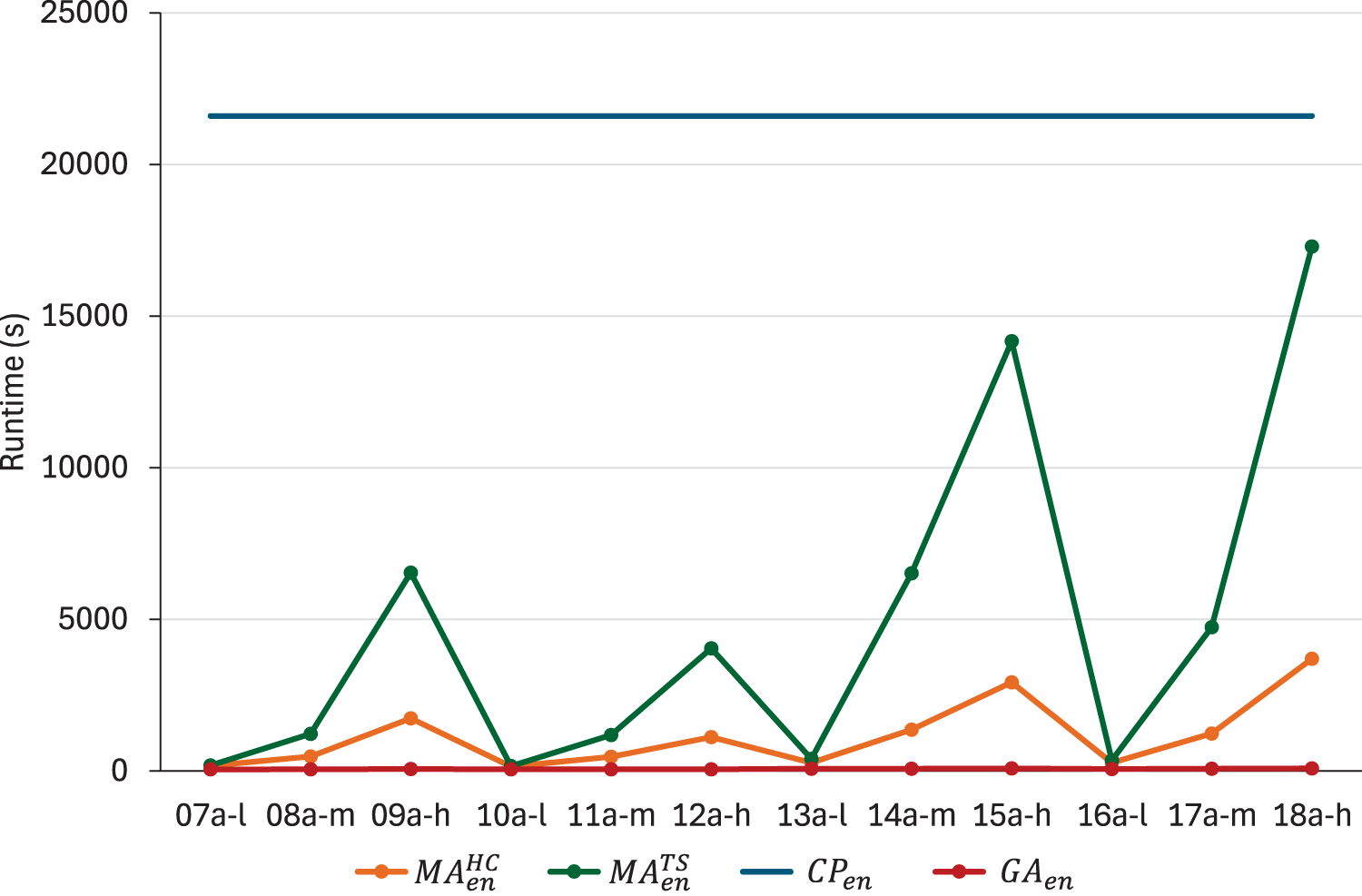
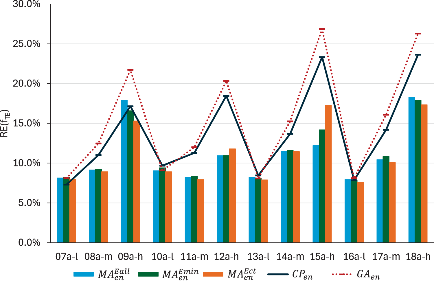
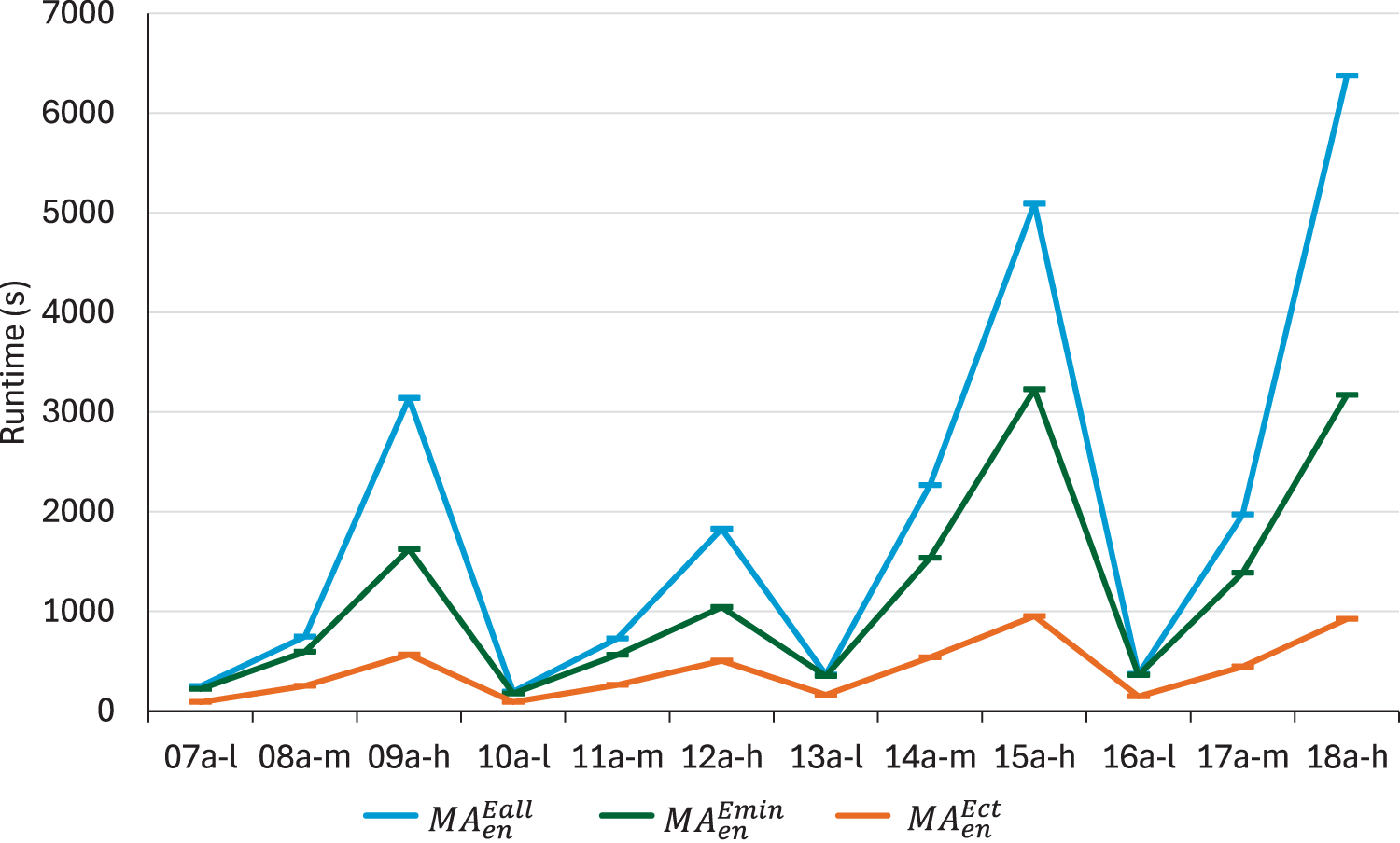
Regarding energy optimisation, Figures 4 and 5 illustrate that both $M{A}_{en}$ versions of the algorithm outperform $G{A}_{en}$ , as above. While this improvement is not as pronounced as that observed in makespan, it still ranges from 17% to 55% in medium and high flexibility instances. What is more important, $M{A}_{en}$ reaches better results than the upper bound obtained by solving the $C{P}_{en}$ model in most instances, especially in higher flexibility ones. When comparing both $M{A}_{en}$ strategies, $M{A}_{en}^{TS}$ appears to obtain smaller relative errors than $M{A}_{en}^{HC}$ in the majority of instances. As in the case of makespan minimisation, we consider that the reduction in quality is not sufficient to offset the high computational resource consumption, which can reach up to 5 hours. Therefore, in terms of energy consumption, $M{A}_{en}^{HC}$ is also a preferable option.

To enhance readability, we shall remove the superscripts from the method’s name in the following sections.

5.5.2. Neighbourhood structure

Once the local search strategy has been set to Hill Climbing, the neighbourhood structure that is most appropriate for each objective will be identified through this analysis.

First, we focus on makespan optimisation. Figure 6 depicts the $RE(f_{C_{max}})$ values reached by $M{A}_{ms}$ using the three proposed neighbourhoods for ${\mathbf{C}}_{\mathbf{m}\mathbf{a}\mathbf{x}}$ : reassigning critical tasks to other machines ( $N^{Mmac}$ ), swapping critical arcs at the extremes of critical blocks ( $N^{Mct}$ ) and the union of both neighbourhoods ( $N^{Mall}=N^{Mmac}\cup N^{Mct}$ ). The three memetic algorithms that result from using these neighbourhoods are denoted $M{A}_{ms}^{Mmac}$ , $M{A}_{ms}^{Mct}$ , and $M{A}_{ms}^{Mall}$ , respectively, in this study. The results obtained by $G{A}_{ms}$ and solving $C{P}_{ms}$ are also included for reference. The average runtime in seconds is shown in Figure 7. In terms of quality, $M{A}_{ms}^{Mall}$ is clearly better than the others. Moreover, it is not the most time consuming algorithm, which is $M{A}_{ms}^{Mmac}$ . This can be explained by the use of the estimation filter. The estimation is more realistic in the neighbours from $M{A}_{ms}^{Mct}$ , which allows us to prune the neighbourhood better. In turn, even though $M{A}_{ms}^{Mall}$ is larger than $M{A}_{ms}^{Mmac}$ , it requires less evaluations to find the best neighbour. On the other hand, $M{A}_{ms}^{Mct}$ appears as the fastest, reducing the runtime of $M{A}_{ms}^{Mall}$ by 3 minutes and a half on average. However, the relative errors obtained are significantly worse than those obtained by $M{A}_{ms}^{Mall}$ , even doubling them in some instances with high flexibility. Therefore, given the differences in terms of relative errors, we consider that using $N^{Mall}$ is, overall, the best option to minimise makespan.

Figure 6.

$RE(f_{C_{max}})$ values obtained by $M{A}_{ms}^{Mall}$ , $M{A}_{ms}^{Mmac}$ and $M{A}_{ms}^{Mct}$ .

Figure 7.

CPU times obtained by $M{A}_{ms}^{Mall}$ , $M{A}_{ms}^{Mmac}$ and $M{A}_{ms}^{Mct}$ .

Compared to the version of the algorithm without local search, $G{A}_{ms}$ , we see a clear improvement when intensification is applied using $N_{all}$ . The improvement increases with flexibility, going from an average reduction of 4.9% in type $l$ instances to 8.3% in type $m$ instances and 11.5% in type $h$ instances. Regarding solving $C{P}_{ms}$ , the memetic algorithm reaches solutions that are slightly worse in quality, as expected, but it takes less than 8 minutes on average compared to the 6 hours required by the CP method.

In terms of energy optimisation, we also compare the three proposed neighbourhood structures to minimise $\mathbf{T}\mathbf{E}$ : reassigning any task to a machine where it consumes less energy ( $N^{Eall}$ ), reassigning a critical task to a machine where it consumes less energy ( $N^{Ect}$ ) and reassigning any task to the machine where it consumes the least amount of energy ( $N^{Emin}$ ). Following the previous notation, we shall denote the three resulting memetic algorithms as $M{A}_{en}^{Eall}$ , $M{A}_{en}^{Ect}$ and $M{A}_{ms}^{Emin}$ respectively. In Figure 8 we can see that no algorithm outperforms the others for every instance in terms of $RE(f_{TE})$ . $M{A}_{en}^{Ect}$ reaches the best relative error in all but two instances: 12a-h and 15a-h, where it is actually the worst. But in most of the instances, there are not significant differences between the three algorithms. However, this is not the case when comparing runtimes. In instances with high flexibility, the CPU times used by $M{A}_{en}^{Ect}$  as can be seen in Figure 9 are one order of magnitude smaller than those used by $M{A}_{en}^{Eall}$ , and significantly better than those obtained with $M{A}_{en}^{Emin}$ . This makes sense: higher flexibility means that there are more candidate machines to reassign a task to and, consequently, more neighbours to explore. However, since the $N^{Ect}$ neighbourhood is restricted to critical tasks only, its size is much less affected by flexibility.

Figure 8.

$RE(f_{TE})$ values obtained by $M{A}_{en}^{Eall}$ , $M{A}_{en}^{Emin}$ and $M{A}_{en}^{Ect}$ .

The change in neighbourhood may affect the choice of the search strategy made in the previous subsection. To verify if this is the case, an additional experiment has been conducted comparing again $M{A}_{en}^{HC}$ and $M{A}_{en}^{TS}$ using the new neighbourhood, $N_{en}^{Ect}$ . The results are in line with those obtained previously, so we have maintained the choice of using Hill Climbing Figure 9. The results also show the benefits of using local search versus not using it ( $G{A}_{en}$ ). When choosing the $N^{Ect}$ neighbourhood, we cannot appreciate a significant improvement in low-flexibility instances ( $l$ ). But for the type- $m$ ones, there is an average reduction of $RE$ of 4.4%, which increases to 8.4% in type- $h$ instances. What is more remarkable is that the memetic algorithm gets similar results to solving $C{P}_{en}$ in type- $l$ instances, but it is significantly better in instances with higher flexibility.

Figure 9.

CPU times obtained by $M{A}_{en}^{Eall}$ , $M{A}_{en}^{Emin}$ and $M{A}_{en}^{Ecp}$ .

In summary, we setup our lexicographic method by using Hill Climbing with $N_{ms}^{Eall}$ when the solution does not meet the makespan goal and Hill Climbing with $N^{Ect}$ when it does. Notice that the energy-oriented neighbourhood is only used on solutions with a good makespan value. This may affect the number of neighbours considered and, therefore, the number of good candidate solutions to evaluate. If this decreases enough, one may think that Tabu Search could become viable in this setting, and even the use of the larger neighbourhood $N_{en}^{Eall}$ . We have tested this and the results obtained show that using Hill Climbing with $N_{en}^{Ect}$ is 86.1% faster than using Tabu Search with $N_{en}^{Eall}$ , while sacrificing only 0.5% of $RE(f_{TE})$ . Therefore, we consider that Hill Climbing with $N_{en}^{Ect}$ is also the best option for energy-oriented local search in the lexicographic setting.

5.6. Lexicographic analysis

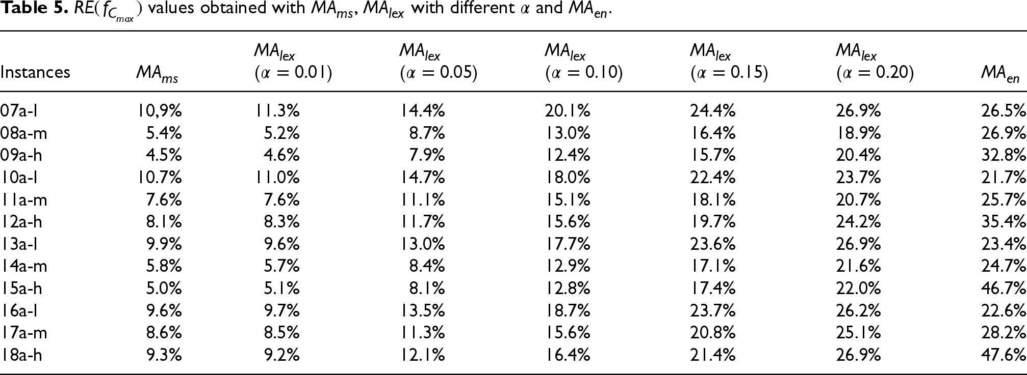
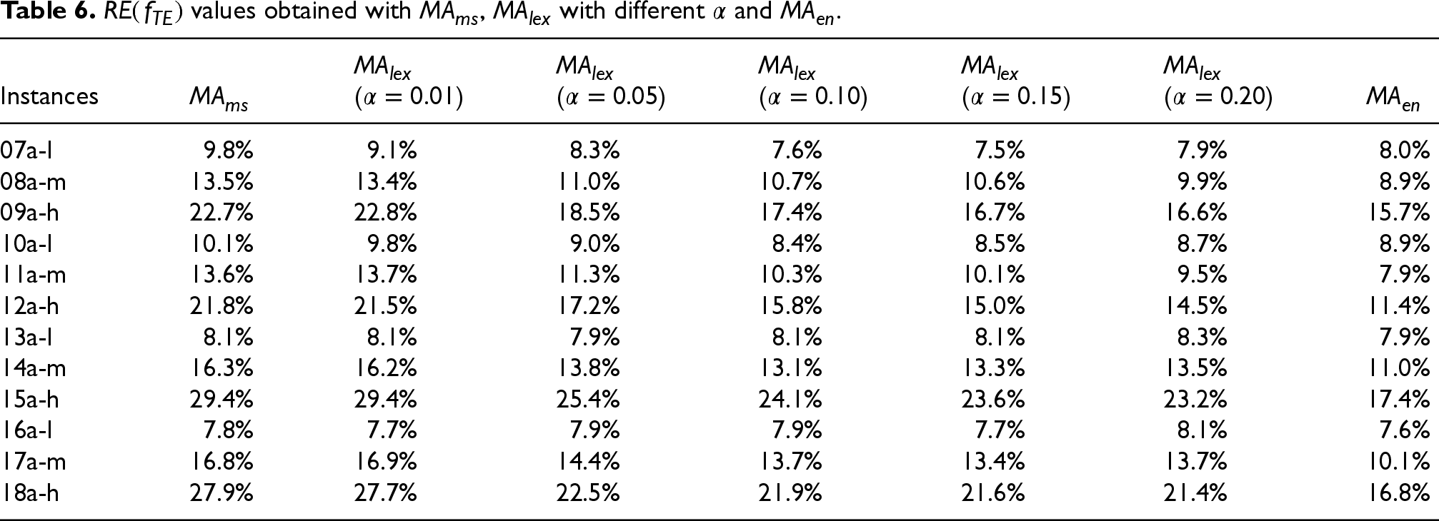
Once the best setup for the algorithm has been chosen, we test its performance in this section. Tables 5 and 6 report, respectively, the relative errors for ${\mathbf{C}}_{\mathbf{m}\mathbf{a}\mathbf{x}}$ and $\mathbf{T}\mathbf{E}$ obtained with $M{A}_{lex}$ . We include results obtained with different $\alpha$ values for the makespan goal. For comparison, we also report the $RE$ obtained by the single-objective versions, $M{A}_{ms}$ and $M{A}_{en}$ , after their tuning in the previous subsection. For these versions, we drop the superscript previously used for simplicity.

Table 5.

$RE(f_{C_{max}})$ values obtained with $M{A}_{ms}$ , $M{A}_{lex}$ with different $\alpha$ and $M{A}_{en}$ .

		$M{A}_{lex}$	$M{A}_{lex}$	$M{A}_{lex}$	$M{A}_{lex}$	$M{A}_{lex}$
Instances	$M{A}_{ms}$	( $\alpha =0.01$ )	( $\alpha =0.05$ )	( $\alpha =0.10$ )	( $\alpha =0.15$ )	( $\alpha =0.20$ )	$M{A}_{en}$
07a-l	10,9%	11.3%	14.4%	20.1%	24.4%	26.9%	26.5%
08a-m	5.4%	5.2%	8.7%	13.0%	16.4%	18.9%	26.9%
09a-h	4.5%	4.6%	7.9%	12.4%	15.7%	20.4%	32.8%
10a-l	10.7%	11.0%	14.7%	18.0%	22.4%	23.7%	21.7%
11a-m	7.6%	7.6%	11.1%	15.1%	18.1%	20.7%	25.7%
12a-h	8.1%	8.3%	11.7%	15.6%	19.7%	24.2%	35.4%
13a-l	9.9%	9.6%	13.0%	17.7%	23.6%	26.9%	23.4%
14a-m	5.8%	5.7%	8.4%	12.9%	17.1%	21.6%	24.7%
15a-h	5.0%	5.1%	8.1%	12.8%	17.4%	22.0%	46.7%
16a-l	9.6%	9.7%	13.5%	18.7%	23.7%	26.2%	22.6%
17a-m	8.6%	8.5%	11.3%	15.6%	20.8%	25.1%	28.2%
18a-h	9.3%	9.2%	12.1%	16.4%	21.4%	26.9%	47.6%

Table 6.

$RE(f_{TE})$ values obtained with $M{A}_{ms}$ , $M{A}_{lex}$ with different $\alpha$ and $M{A}_{en}$ .

		$M{A}_{lex}$	$M{A}_{lex}$	$M{A}_{lex}$	$M{A}_{lex}$	$M{A}_{lex}$
Instances	$M{A}_{ms}$	( $\alpha =0.01$ )	( $\alpha =0.05$ )	( $\alpha =0.10$ )	( $\alpha =0.15$ )	( $\alpha =0.20$ )	$M{A}_{en}$
07a-l	9.8%	9.1%	8.3%	7.6%	7.5%	7.9%	8.0%
08a-m	13.5%	13.4%	11.0%	10.7%	10.6%	9.9%	8.9%
09a-h	22.7%	22.8%	18.5%	17.4%	16.7%	16.6%	15.7%
10a-l	10.1%	9.8%	9.0%	8.4%	8.5%	8.7%	8.9%
11a-m	13.6%	13.7%	11.3%	10.3%	10.1%	9.5%	7.9%
12a-h	21.8%	21.5%	17.2%	15.8%	15.0%	14.5%	11.4%
13a-l	8.1%	8.1%	7.9%	8.1%	8.1%	8.3%	7.9%
14a-m	16.3%	16.2%	13.8%	13.1%	13.3%	13.5%	11.0%
15a-h	29.4%	29.4%	25.4%	24.1%	23.6%	23.2%	17.4%
16a-l	7.8%	7.7%	7.9%	7.9%	7.7%	8.1%	7.6%
17a-m	16.8%	16.9%	14.4%	13.7%	13.4%	13.7%	10.1%
18a-h	27.9%	27.7%	22.5%	21.9%	21.6%	21.4%	16.8%

As expected, Table 5 shows that $M{A}_{ms}$ obtains the best solutions in terms of makespan and $M{A}_{en}$ obtains the worst. Conversely, Table 6 shows that $M{A}_{en}$ gets the best results for energy optimisation and $M{A}_{ms}$ , the worst. However, we can see that the room for improvement is much larger in makespan and it highly depends on the flexibility of the instances. When minimising ${\mathbf{C}}_{\mathbf{m}\mathbf{a}\mathbf{x}}$ , the difference in low flexibility instances goes from an average 23.6% RE obtained by $M{A}_{en}$ to 10.3% when using $M{A}_{ms}$ : 13.6% difference. This value increases to 19.5% in medium flexibility instances (26.4% vs. 6.9%) and 33.9% in high flexibility instances (40.6% vs. 6.7%). Similarly, when minimising $\mathbf{T}\mathbf{E}$ the differences are 0.8% for $l$ -type instances, 5.6% for $m$ -type ones and 10.1% for $h$ -type ones. In this case, in favour of $M{A}_{en}$ . The reason for this behaviour is that, when more machines are available to execute each task, the energy consumption can be reduced by waiting for the machine with the lowest energy consumption for each task. Obviously, this has a big impact on the makespan. This happens is especially relevant in our model, where machines are turned on when starting executing the first assigned task, so delaying their execution to wait for the most energy-efficient machine does not increase the consumed passive energy too much.

The lexicographic memetic algorithm, due to its nature, is focused first on reaching the makespan goal. But what is more important in our algorithm is that, when the goal is relatively easy to reach, it is capable of finding solutions with energy consumptions close to those obtained when minimising only this objective function. We can appreciate this behaviour by looking at the different columns for $M{A}_{lex}$ , where the goal is easier to achieve the larger the value of $\alpha$ . It can be appreciated that with $\alpha =0.01$ , the improvement in energy consumption is small compared to not considering it ( $M{A}_{ms}$ ). However, with $\alpha =0.05$ , the solutions are very close to those obtained by $M{A}_{en}$ in terms of energy consumption.

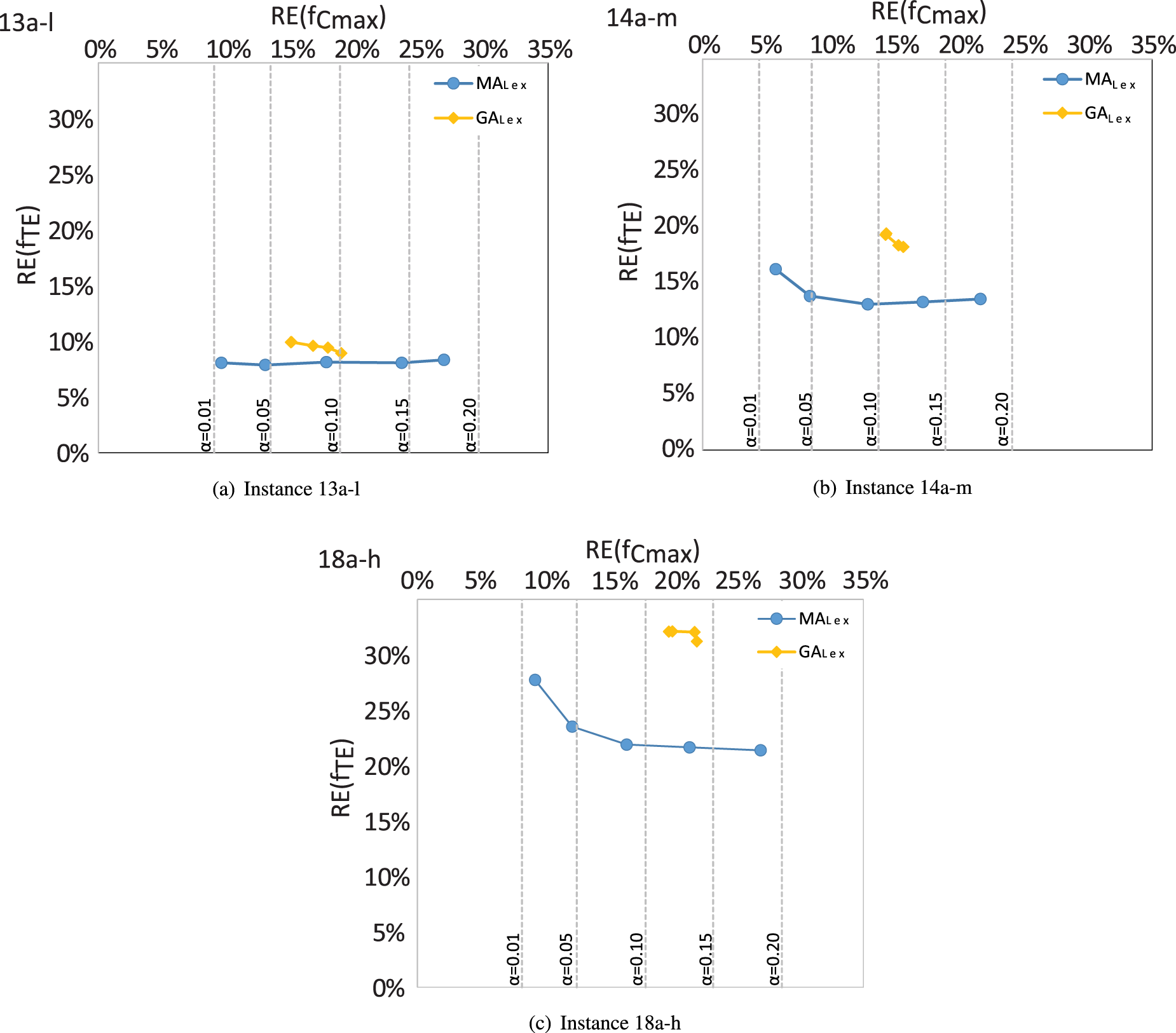
To better illustrate this, we plot the results of $M{A}_{lex}$ for different values of $\alpha$ in Figure 10. An instance of each flexibility level is depicted. The leftmost point of each line represents $\alpha =0.01$ and increases to $\alpha =0.20$ at the rightmost point. We also include the state-of-the-art results for our problem obtained by a $GA$ . ⁶⁶ We can see that the proposed $M{A}_{lex}$ is capable of reaching the makespan goal for all values of $\alpha$ except 0.01, while $G{A}_{lex}$ can barely reach it when $\alpha =0.10$ and the flexibility is medium or high. Most importantly, $M{A}_{lex}$ leads to a reduction in total energy consumption in all instances and values of $\alpha$ . It seems that, when the goal is relaxed, $M{A}_{lex}$ reaches it easily and, from that point, focusses its effort on optimising $\mathbf{T}\mathbf{E}$ , as expected. Meanwhile, $G{A}_{lex}$ struggles to optimise the energy without losing the makespan goal even when it can reach it. As a consequence, it loses the ability to keep the makespan close to its goal while decreasing $\mathbf{T}\mathbf{E}$ . This behaviour can be observed across all instances.

Figure 10.

$RE(f_{{\mathbf{\text{C}}}_{max}})$ and $RE(f_{TE})$ obtained in different flexibility type instances using $G{A}_{lex}$ , $M{A}_{lex}$ with varying $\alpha$ values. Corresponding goals are shown as vertical dashed lines.

6. Conclusion

In this study, we address flexible job shop problem with interval processing times considering two objectives: minimising makespan and total energy consumption. Despite having two objective functions, there is a clear hierarchy between them. It is desirable to consume less energy; however, a certain quality of service should be guaranteed in the first place. Therefore, minimising makespan is the primary objective, but after it reaches a certain level, we can focus on minimising the total energy consumption. To address this problem, a lexicographic goal programming approach is adopted.

A memetic algorithm, which is composed of a genetic algorithm combined with a local search, is developed to solve our problem. Local search algorithms entail defining neighbourhood structures. In this work, three different neighbourhoods are established and tested for each objective along with two local search methods: hill climbing and tabu search. After testing the neighbourhoods and the local search methods in the mono-objective cases, the most adequate options are selected.

In this memetic algorithm, a dynamic strategy is implemented that allows to choose the neighbourhood depending on the objective that is being optimised at each step. Firstly, it focusses on reaching the makespan goal by using the makespan-oriented neighbourhoods. Once this goal is achieved, the method switches to energy-oriented neighbourhoods to minimise the second objective. Moreover, to speed up the local search, we provide easy-to-compute estimates for each objective value that enable faster evaluation of neighbours and pruning the neighbourhood without compromising quality.

Our experimental results indicate that the proposed algorithm reaches the makespan goal in many more cases compared to previous methods. Moreover, the new method behaves more accordingly to expectations: once the makespan goal is reached, it stops putting effort into that objective function and instead it greatly minimises the total energy consumption. This impact is even more obvious for instances with higher flexibility, which are significantly harder due to their larger solution spaces.

Green flexible job shop scheduling with interval processing times is a new and fast-growing research field, and there remain many questions to be answered. One of the potential future research directions could involve evaluating the robustness of the solutions found under uncertainty. Furthermore, it would be interesting to develop new solution methods that combine different algorithms to increase solution quality without compromising efficiency. Finally, incorporating more sophisticated power use models that take more realistic properties into account (such as power spikes at machine activation or time-varying power use) would increase the applicability of these models in real-life scenarios.