Sage Journals: Discover world-class research

Abstract

Many insects use view-based navigation, or snapshot matching, to return to familiar locations, or navigate routes. This relies on egocentric memories being matched to current views of the world. Previous Snapshot navigation algorithms have used full panoramic vision for the comparison of memorised images with query images to establish a measure of familiarity, which leads to a recovery of the original heading direction from when the snapshot was taken. Many aspects of insect sensory systems are lateralised with steering being derived from the comparison of left and right signals like a classic Braitenberg vehicle. Here, we investigate whether view-based route navigation can be implemented using bilateral visual familiarity comparisons. We found that the difference in familiarity between estimates from left and right fields of view can be used as a steering signal to recover the original heading direction. This finding extends across many different sizes of field of view and visual resolutions. In insects, steering computations are implemented in a brain region called the Lateral Accessory Lobe, within the Central Complex. In a simple simulation, we show with an SNN model of the LAL an existence proof of how bilateral visual familiarity could drive a search for a visually defined goal.

Keywords

Snapshot navigation insect navigation active vision visual familiarity central complex neuromimetics visual compass route-following

1. Introduction

Visual navigation is essential for many animals and has increasing usage in artificial systems, as it presents a cheap way to provide egocentric spatial information for application in autonomous agents. Effective visual navigation algorithms enable autonomous agents to explore and navigate environments without external control. In contrast to methods such as Simultaneous Localization and Mapping (SLAM, (Bresson et al., 2017; Chen et al., 2021; Gridseth & Barfoot, 2021; Smith & Cheeseman, 1986)), insect inspired view-based navigation models derive from agents with poor visual resolution (1°–4°, (Schwarz et al., 2011)) and computationally restricted hardware (ants have fewer than ∼500,000 neurons in their brain (Godfrey et al., 2021)). Thus, mimicking insect behaviours and computational principles may overcome hardware limitations and increase not only computational efficiency but, given the navigational prowess of insects, also help with the robustness of applied navigation mechanisms in dynamic environments.

Behavioural experiments and modelling of visual landmark learning in bees (Cartwright & Collett, 1983) sparked the subsequent development of several view-based navigation algorithms (Chahl & Srinivasan, 1996; Franz, 1998; Moeller & Vardy, 2006; Smith et al., 2007). With view-based navigation, an environment can be sparsely represented with reference images (snapshots) taken at nodes relevant for navigation within the environment. For instance, navigation to a node can happen via gradient descent, as the image difference can be used as an indicator for proximity to a goal location (Zeil et al., 2003). By calculating the root mean square pixel difference between memorised panoramic snapshots and query images from displaced locations in the vicinity, a spatial Image Difference Function (IDF) can be established (under the condition that all images have the same heading). This function is minimal when the query image is in the same location as the memorised snapshot but gradually increases with distance to that memorised snapshot’s location. By following the descending gradient, the location of the memorised snapshot can be found.

The measure of visual difference can also be directly incorporated into an algorithm for setting orientation as part of homing algorithms. One set of methods uses the concept of a ‘visual compass’ (Labrosse, 2006; Stuerzl et al., 2008; Zeil et al., 2003), which is a method to find the best matching orientation between a memorised snapshot and a query image, therefore leading to the recovery of the heading at which the memorised snapshot was stored, also called a rotary Image Difference Function (rIDF). Systematic rotational sampling, in order to find the best match with a stored shapshot, resembles the behaviour of ants which scan the environment with body rotations while visually navigating (Lent et al., 2010; Wystrach et al., 2014), leading to a stop-scan-go movement. Such visual compass algorithms are good at explaining the route navigation behaviours of ants (Collett et al., 2013; Narendra, 2007; Philippides et al., 2011; Zeil, 2012), where routes can be established by memorising snapshots along a path to be navigated along. The memorised snapshots can be stored either as they are (‘Perfect Memory’) or by feeding them into a holistic memory creation mechanism, such as the machine learning algorithm ‘Infomax’. The Infomax algorithm creates one holistic memory from all memorised snapshots, memorising effectively the most different snapshots from the whole set of memorised snapshots (Baddeley et al., 2012; Wystrach et al., 2013).

Algorithms that rely on whole-body rotation or mental rotation (Husbands et al., 2021; Moeller, 2012) to evaluate possible directions of travel can be computationally or time intensive. Therefore, it is interesting to look in detail at the active scanning behaviours of insects to make Snapshot navigation even more efficient. Based on the observation that ants move in sinusoidal trajectories, Kodzhabashev and Mangan replaced the stop-scan-go movement strategy with a sinusoidal movement pattern, where the amplitude is modulated by the memorised snapshot familiarity. This leads to a high-amplitude sinusoidal movement with weak input familiarity and a shallow sinusoidal movement with strong familiarity, enabling a robot to navigate along a route (Kodzhabashev & Mangan, 2015). Therefore, the scanning movement is spread out over several movement steps and makes the familiarity following process more dynamic.

In insects, rhythmic motor patterns are produced by a specific brain area called the Lateral Accessory Lobe (LAL). The LAL is a conserved brain structure, which receives inputs from learning and sensory centres and connects with the motor centres. It consists of two lobes, one located in each brain hemisphere. The inputs are largely divided hemispherically, meaning that the inputs towards one lobe mainly originate in the same hemisphere (Namiki et al., 2014) and subsequent processing occurs predominantly within the same hemisphere also (Paulk et al., 2015). Behaviourally, the LAL seems to be involved in the generation of small-scale search behaviours (Kanzaki et al., 1992; Pansopha et al., 2014). These seem to be modulated by the reliability of navigation cues (which may be encoded by the strength of the incoming signal (Deneve et al., (2000)), leading to extensive search for a cue if that cue is weakly perceived, and targeted steering behaviours when the cue is strong (Namiki & Kanzaki, 2016; Steinbeck et al., 2020). Steering is achieved by an imbalance of activity of descending neurons towards the motor centres (Iwano et al., 2010; Rayshubskiy et al., 2020; Zorovic & Hedwig, 2013). Because this appears to be a general purpose circuit in insects, we have recently developed a steering framework based on the LAL (Steinbeck et al., 2020), which provides a general mechanism for sensory information to control orientation and active search.

Based on the steering framework, where hemispherically divided inputs ultimately lead to a steering response, we investigate how bilaterally organised visual memories could achieve a steering response to navigate along a learned route. Instead of using a single panoramic image as a memory, as for many of the models above, we use two lateralised memories. This is biologically plausible given the lateralised wide field eyes and the bilateral Mushroom Bodies, which are the site of visual route memories (Buehlmann et al., 2020; Kamhi et al., 2020; Li et al., 2020; Liu et al., 1999; Vogt et al., 2014). Such lateralised use of sensory information is reminiscent of Braitenberg’s Vehicles, wherein adaptive behaviour in some of his hypothetical automomous agents was produced by lateralised sensori-motor connections (Braitenberg, 1984). Our characterisation of the LAL (Steinbeck et al., 2020) shares with Braitenberg’s vehicles the principle that rich behaviours can emerge from relatively simple sensory-motor connections when the agent is tuned to the correct environmental information.

Given the LAL controls steering by using the strength of lateralised sensory inputs, we ask how the organisation of bilateral view-based memories can be optimised to provide a reliable steering signal. The investigation mainly focuses on the Field of View (FoV), which describes how much raw visual information is available to each hemispheric memory, and an Offset, which describes the target/familiar orientation of the stored memories in relation to the agent’s heading, which has been applied similarly in Wystrach et al. (2020). The spontaneous difference in visual familiarity between the current and stored views for both hemispheres is used as a steering signal, similar to a taxis mechanism. In sum, we explore which Fields of View would fit best with this steering process and therefore would be a biological plausible input to the insect LAL during navigation.

2. Methods

Modelling and analyses were performed with MATLAB 2017 and 2019 (The MathWorks, Inc, Natick, MA, USA). The code to run the simulations and analysis as described in the methods can be found online at https://github.com/FabianSteinbeck/FamiliarityTaxis.

2.1. Antworld image rendering

For the exploration of Bilateral Snapshot navigation we chose to use the ‘Antworld’ virtual environment, which is an LiDAR (Light Detection And Ranging) 3-D reconstruction of an experimental location, near Seville Spain, which has been used for observations and experiments with Cataglyphis velox ants (Risse et al., 2018). Within this environment, we chose two routes which closely resemble real routes taken by ant foragers navigating towards their nest (routes 3 and 12 from the Brains on Board (BoB) robotics GitHub (https://github.com/BrainsOnBoard/bob_robotics/tree/master/resources/antworld), Figure 1(a)). The rendering of the test images is done with the BoB robotics Antworld rendering pipeline (https://github.com/BrainsOnBoard/bob_robotics/tree/master/python/antworld, an adaptation from Risse et al., 2018, see https://insectvision.dlr.de/3d-reconstruction-tools/habitat3d). To generate training views and displaced test locations, on each route we chose 31 equally spaced locations (a 6.2 m long path, each location 0.2 m apart and at 17.5 mm height, due to uneven ground and therefore avoiding rendering ‘under ground’), where the centre of the panoramic image (heading for the agent) faces towards the next location. These are the training locations for the memorised snapshots. For testing, at each location we rendered five off-route locations normal to the route direction, both to the left and right (distances were 5, 10, 30, 100 and 300 mm; Figure 1(d)). The panoramic images are rendered so that the centre pixels represent the heading direction, that is, the view orientation oscillated about the overall route direction.

Figure 1.

Visual environment “Antworld” simulating a desert-like environment with sparse vegetation. A top-down view of the virtual environment (a), showing Route 3 from the BoB robotics GitHub (red) and the off-route test locations (blue) (d). The two locations singled out show the view from along the route (b) and displacements to the side of the route (c) at different visual resolutions.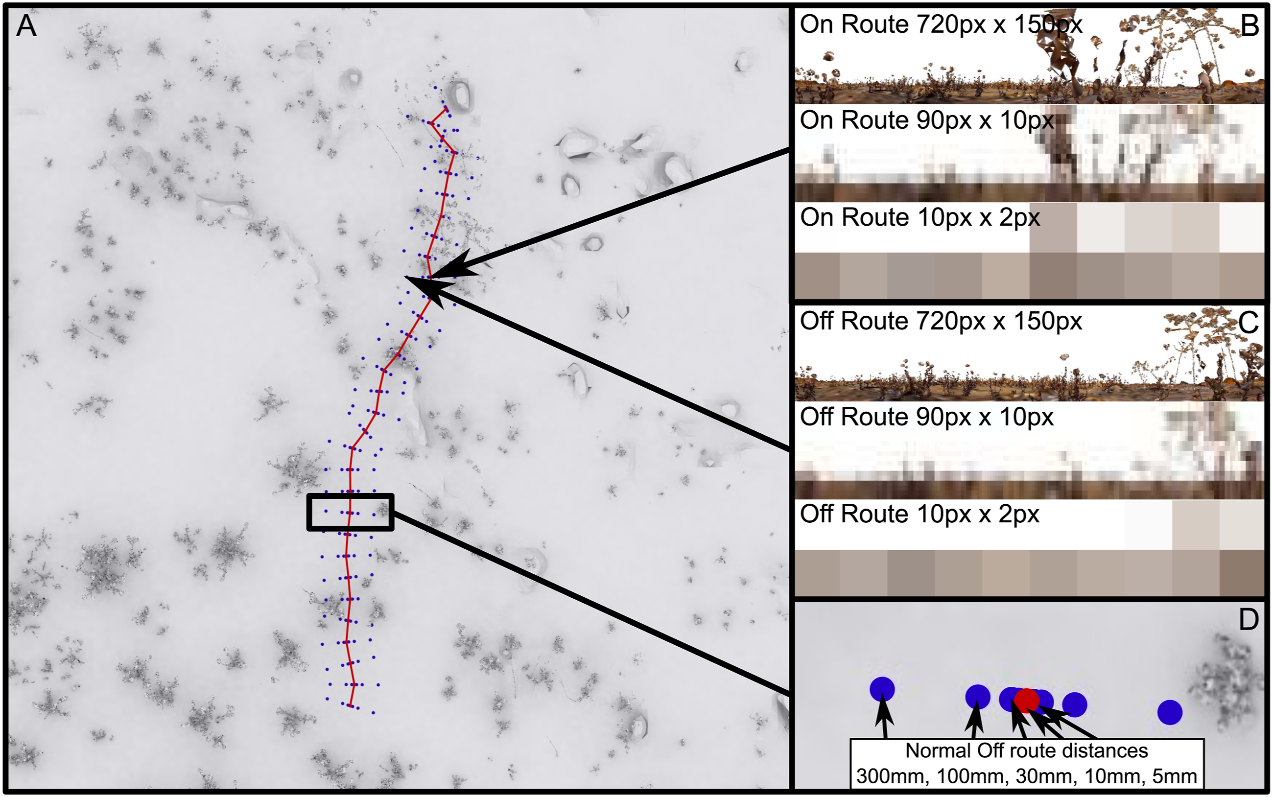

2.2. Field of view

The field of view (FoV) describes the visual input available to each hemisphere/eye, which is then both used for memorised snapshots and the comparison of the query images to the memorised snapshots to generate the rotary Image Familiarity Function (rIFF). Because both hemispheres/eyes have a field of view, visual systems are further described by the degree of visual overlap (the visual range of both eyes overlapping in the front) and the size of the rear blindspot (how much visual range is missing to the back). A panorama’s central horizontal pixel is the heading direction; therefore, the blindspot refers to how many pixels are taken away from the edges of the image, as the edges of the image are in the opposite direction to the heading direction. The overlap defines how many pixels are designated to be taken beyond the horizontal centre contralaterally for each of the images. For our experiments, we set up a range of differently sized and oriented FoVs (see Table 1).

Table 1.

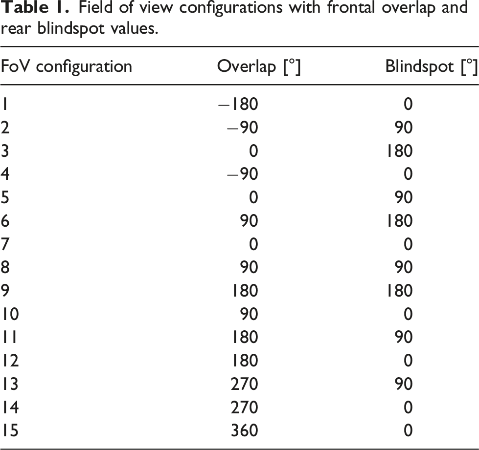
Field of view configurations with frontal overlap and rear blindspot values.

FoV configuration	Overlap [°]	Blindspot [°]
1	−180	0
2	−90	90
3	0	180
4	−90	0
5	0	90
6	90	180
7	0	0
8	90	90
9	180	180
10	90	0
11	180	90
12	180	0
13	270	90
14	270	0
15	360	0

2.3. Offset

The Offset describes the orientation of a memorised snapshot in relation to an agent’s body and to the overall route direction. If a view is stored with no Offset, this would mean that the most familiar direction is directly aligned with the agent’s overall direction of travel. An Offset angle for each FoV would mean that agents memorised a view when the body was rotated away by the Offset angle relative to the overall trajectory direction (Figure 2(c)). This would result in maximally familiar directions occurring at angles symmetric to the agent’s centre line. For example, an Offset of 45° would result in the left FoV having a maximum familiarity when the agent was rotated by 45° to the right from the original heading direction and the overall route direction from the training images, and vice versa (Figure 2(c)). For convenience within the setup of this experiment, this is achieved by rotating the panoramic query image for each hemispheric query image before cutting it into the FoV. The Offset values tested were [0°, 9°, 18°, 27°, 36°, 45°, 54°, 63°, 72°, 81°, 90°].

Figure 2.

Impact of Offset on visual familiarity. (a) A panoramic snapshot (720/150 px). (b) The panoramic snapshot divided into two memories (each 360/150 px, a FoV with 0° overlap, 0° blindspot and 0° Offset). (c) left: Representation of when snapshots are taken for zero offset, i.e. when facing route direction; (c) right: Snapshots taken with an Offset θ. (d) left, top: rotary Image Familiarity Functions per eye (yellow = left eye, blue = right eye) generated with the above snapshot/memories with no Offset. (d) left, bottom: the difference between left and right eye familiarity functions. (d) right: the same depictions, but for snapshots with an Offset.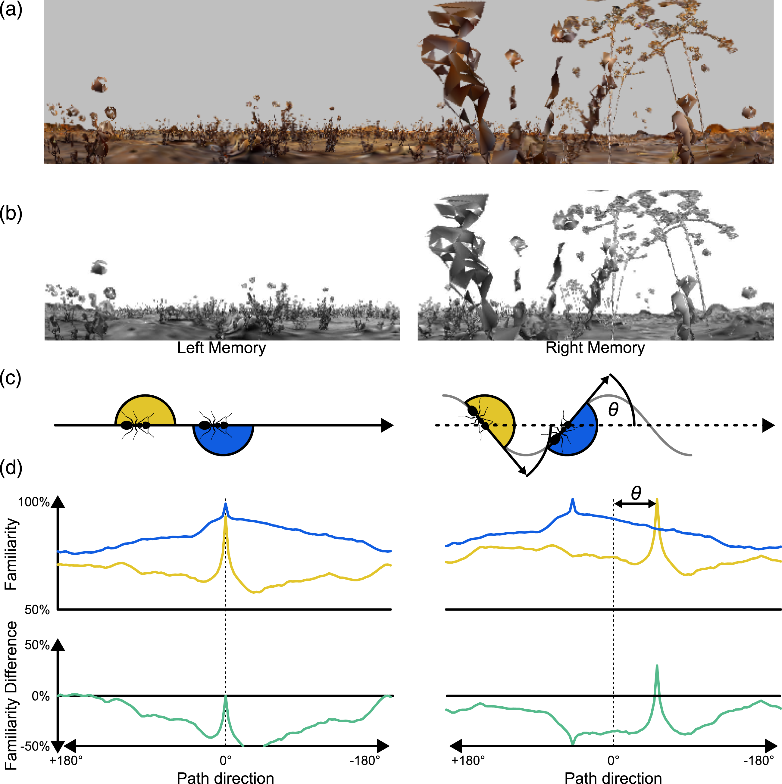

2.4. Image processing

The images are processed with the following steps:

• the panoramic images are rendered over 360° x-Axis and 180° y-Axis, with 720 pixels in the x-Axis and 150 pixels in the y-Axis (720/150), which is .5 °/px in the x-Axis and 1.2°/px in the y-Axis;

• the sky’s colour is made white;

• the whole image is converted to gray-scale;

• each image is then cut into two views, depending on the specific FoV and Offset for that test (see Table 1 and the code on GitHub);

• for investigations on the impact of resolution, images are downsampled to 90/10, 60/8, 30/6, 20/4 and 10/2 resolutions usingMATLAB’s imresize-function (see Figure 1(b)).

For the main analysis we use 90/10, which gives a resolution comparable to the visual resolution of the ant compound eye (Schwarz et al., 2011).

2.5. Rotary Image Familiarity Function

The rotary Image Familiarity Function (rIFF) is used to systematically compare a memorised snapshot with a series of rotated versions of the ‘current’ query image in order to find which orientation is the most familiar, that is, the best match. The query image is rotated in steps through 360°, at each rotation step (3° for the 720 px image size, 1 pixel step for the smaller image sizes [4°, 6°, 12°, 18°, 36°]) the views for both eyes are extracted from the full panorama and then, with the given FoV (see Table 1), the covariance (familiarity) of each eye’s query image is calculated for the appropriate memorised ipsilateral snapshot (Kagioulis et al., 2020; Wang et al., 2004). Plotting the covariance for the whole 360° gives the rIFF, one for each hemisphere (Figure 2(d)).

2.6. Measures of successful steering

Here, the displaced off-route images are compared to the on-route images at the nearest location. At each location, the rIFFs of the left hemisphere and right hemisphere are individually normalised to their max − 105% · min percentile before being subtracted from each other. This gives us a familiarity difference between left and right eyes which can be used to drive a steering response. Positive values suggest a leftwards turn and negative values indicate steering rightwards. Examples where the familiarity difference gives a correct steering response are given in Figure 2(d).

In order to assess the overall success of a given set of visual system parameters, we take the proportion of orientations, across all test locations, where the Left–Right difference in visual familiarity would indicate a correct turn response. We initially look at this for all orientations, that is, for ±180° from the ‘correct’ direction. However, the main focus of this article is to consider how a bilateral familiarity metric can work for route guidance, in the context of the insect LAL brain region which modulates motor behaviour between steering and search. Therefore, for much of our analysis we focus on the proportion of orientations at test locations that give correct steering responses within ±90° of the current ‘training’ route direction. This gives us an appreciation of how likely the bilateral familiarity information would be in keeping an agent on the desired route, rather than relying on a search behaviour (see introduction).

2.7. Evaluation of aliasing

The memories of a route represent a sequence of experienced views along a route, and ideally the current view experienced by an agent trying to navigate a route would be compared to the correct view in the memorised sequence. However, real world agents might not have access to information that could ensure they compare their current view to the ‘correct’ memorised view. In our scheme agents will use the most familiar view memory, but mistakenly selecting the wrong training view for comparison we will call aliasing, which comes from views from different locations in the environment being similar. To analyse how aliasing might impact on overall correct steering performance, we looked at how the rate of aliasing might vary for different visual parameters. The aliasing metric is derived by considering which of the stored training views give the best match for the current location across all orientations and all possible stored views. This gives us a number for the difference in sequence location between the true best reference location and the position of the apparent best visual match. A score of 2 would mean that the best match for the query image in the query position along the route was 2 positions away from the correct stored image location in the training route sequence of views.

3. Results

3.1. Overall performance of a bilateral visual familiarity method

Our primary goal for this analysis was to give proof of concept that bilateral visual familiarity information can be used to generate a steering signal (Steinbeck et al., 2020). The familiarity signal depends on the comparison of current views to stored route memories. The hypothetical scenario is that an agent has stored left and right eye views along a foraging route and then when trying to navigate using those views, steering will depend on the comparison of left and right visual familiarity. That is, how similar are the current left and right eye views to the stored left and right views. The agent should steer towards the most familiar view, like a taxis mechanism.

In our first analysis, for all orientations at each test location, we evaluate whether the difference in the familiarity between the left and right visual field would lead to a correct steering response. Each pixel of the comparison plot between all visual systems represents one visual configuration (FoV, x-Axis, see Table 1) and Offset (y-Axis) combination, where we aggregate the tests from one route using all on-route and displaced test locations at all orientations. We then show the proportion of these tests (n = [31 on-route locations +31 ⋅ 10 off-route locations] ⋅ 180°/3° rotations = 20,460) where the familiarity difference would give the correct steering response. This performance is only just better than chance when taking into consideration all possible orientations that an agent may find themselves (±180° relative to the heading direction), with 96% getting above 50% correct, but only 1/165 getting 75% correct and none above 80%. Our thresholds here are somewhat arbitrary and reflect the fact that visual navigation is an iterative process without an obligatory cumulative error. Therefore, it is not essential to get every step in exactly the correct direction, but a majority of steering has to be correct. However, our desired behaviour is visual route following. Ants often do not recognise a route instantly, when exposed to reverse route orientations (Schwarz et al., 2017). Thus, we are only taking into consideration the directions ±90° relative to the heading direction. 51/165 (31%) get at least 75% correct and 10/165 (6%) get at least 80% correct. Thus, we have existence proof that there are a range of visual configurations that can generate accurate bilateral familiarity-based steering for view-based navigation along a route.

3.2. Organisation of visual system

The secondary aim of the work was to explore how steering performance depends on the precise organisation of the bilateral visual system. Thus we explored the impact of different field of view sizes, positions and Offsets.

The configurations of FoV and Offset resulting in at least 75% of correct steering responses are found amongst the larger FoVs and non-zero Offsets, 43 out of 165 (26%) visual system configurations at 720/150 px resolution performed over 75% (Figure 3(a), cyan). 80% is reached only with the largest FoVs and medium-to-large Offsets (Figure 3(a), magenta). While the smaller FoV-combinations do not achieve an acceptable performance, those FoV-combinations with bigger blindspots achieve higher performance than with smaller blindspots.

Figure 3.

Steering performance for visual system configurations. (a) Each square represents the proportion of correct steering responses over all tested locations and for orientations within 90° of the overall route direction for a particular visual configuration (x-axis) and Offset (y-axis). The cyan framed pixels surpass 75% and the magenta framed pixels surpass 80% correct steering responses. The blue, red, orange and green dotted columns highlight the visual configurations which are also used in (b). (b) Both top and bottom show performance relative to more granular resolution of Offsets for routes A and B respectively. (c) Proportion of correct steering responses for each orientation, using a visual configuration with 90° Overlap and 90° Blindspot as well as a range of Offsets indicated by the line colours.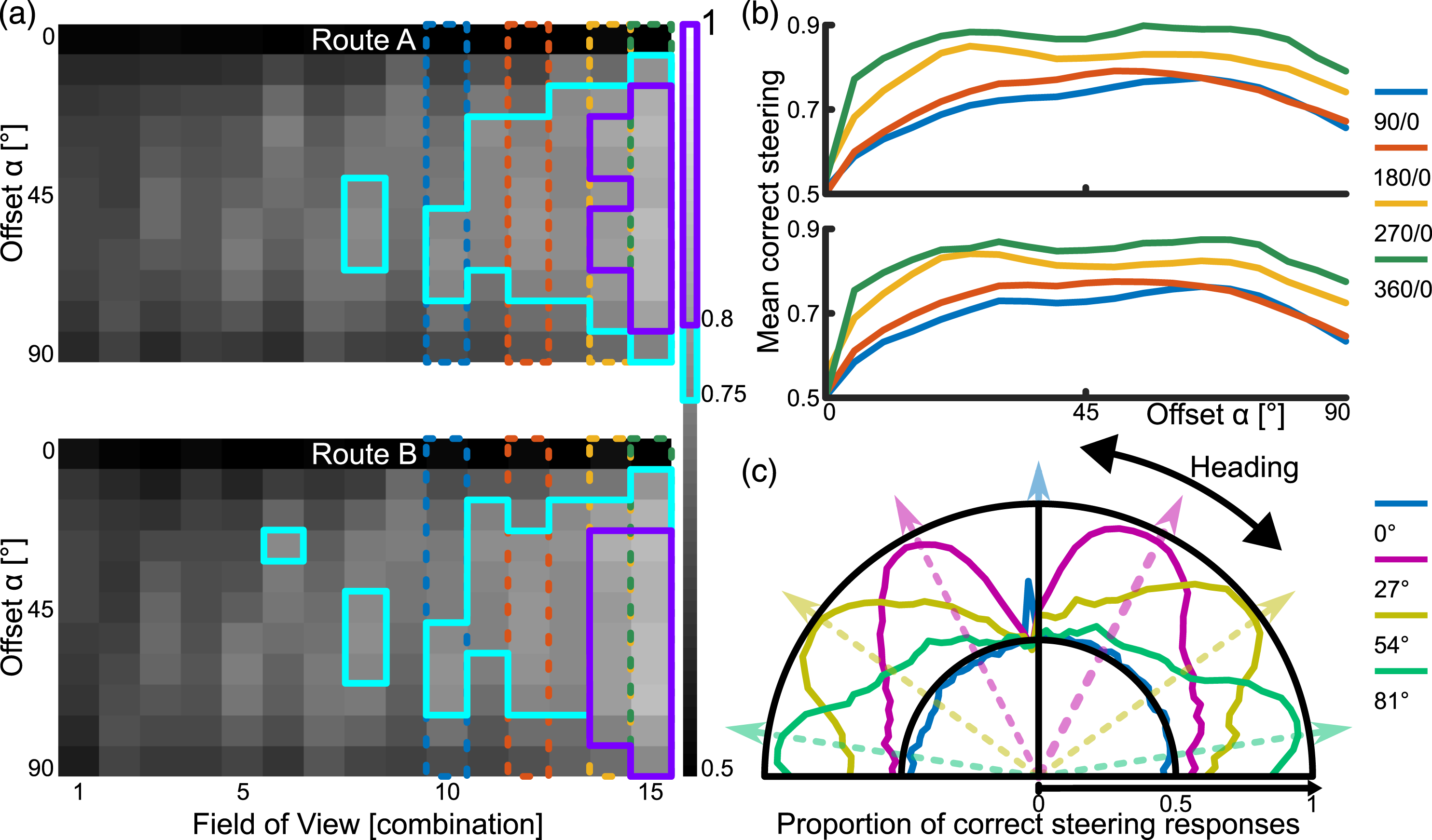

When analysing the influence of the Offset in more detail, it becomes apparent that any Offset other than zero leads to a much improved performance and performance quickly plateaus across a wide range of Offsets (Figure 3(b)). The values fall off towards 90° since the range of considered orientations is ±90°, and for the larger Offsets, correct steering responses may occur beyond this threshold. Investigating in detail how the correct steering responses are distributed for one visual configuration and different Offsets shows how correct steering responses cluster around the Offset angles (Figure 3(c)). That means that the Offset angle plays a crucial role in generating a correct steering response using the difference of familiarity between the left and right view comparisons. A similar result is suggested by Wystrach et al. (2020).

3.3. Visual resolution

Reducing the visual resolution increases the proportion of correct steering responses. 45 out of 165 (27%) visual system configurations performed over 75% with 90/10 px resolution, 53 out of 165 (32%) with 60/8 px resolution, 56 out of 135 (41%) with 30/6 px resolution, 45 out of 90 (50%) with 20/4 px resolution and 34 out of 60 (57%) with 10/2 px resolution. The analyses were performed on two routes, but the pattern of results was very similar, therefore combined them (Figure 4(a)). The increase in performance with reduced resolution matches previous findings regarding using different visual configurations for view-based navigation (Milford, 2013; Wystrach et al., 2016a).

Figure 4.

The impact of visual resolution and aliasing. (a) The correct steering performances for the visual system configurations with different visual resolutions, when using the correct memories. The resolution is shown on top of each image (horizontal resolution/vertical resolution). The cyan framed pixels surpass 75% and the magenta framed pixels surpass 80% correct steering responses. (b) For each visual system configuration we calculated the mean (with standard error) aliasing along the routes, with different visual resolutions. (c) We show the mean (with standard error) aliasing relating to the distance from the route for different visual resolutions.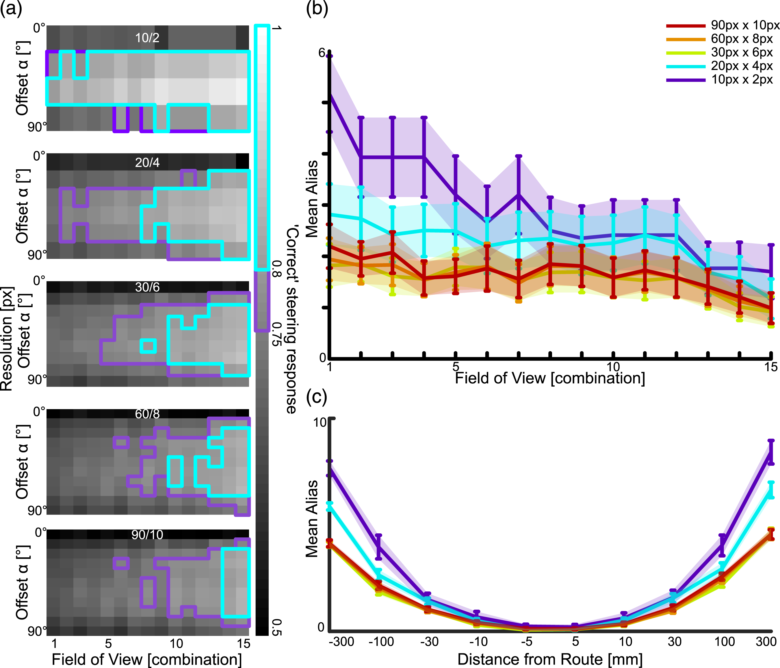

3.4. Aliasing

For our primary analyses, we calculated the familiarity of left and right views using the stored route view that was closest to the test location, that is, the correct view. However, in natural scenarios, when ants are displaced from the route, the best matching view may be a view from an incorrect location at another place along the route, the so called aliasing. We investigated how aliasing depended on visual specification and resolution. Aliasing occurs for all tested configurations but less so for higher resolutions and larger FoVs (Figure 4(b)). Aliasing also increases with displacement distance from the training route (Figure 4(c)). When comparing the query view to the all memories in the memory sequence, instead of the correct one on Route A, the correct steering performance across all visual system configurations reduces to 94% compared to the correct memory performance. This means, the highest familiarity match chosen would be an incorrect view in 6% of cases.

3.5. Central place navigation task

To demonstrate the potential of a bilateral familiarity in a biologically plausible neural model of motor control, we integrated bilateral familiarity information with an LAL model (Steinbeck et al., 2022) for a relatable navigation task, which is navigating towards a central place (see Figure 5). For this, we stored bilateral snapshots from six locations around a central place, each pair facing the central place at a 45° Offset, at three distances (0.5 m, 1 m and 1.5 m), therefore 36 in total. This resembles the images that might be stored following learning walks in ants, where they circle around the nest and periodically look back at it, thereby potentially memorising views of the nest from different directions and distances (Philippides et al., 2013). We generated a grid around that central place spanning 8 m into the horizontal plane with a resolution of .1 m. At each grid location, we calculated the familiarity of each eye individually given the current view and the memorised snapshots. The familiarity values were fed into an LAL-SNN, as described in Steinbeck et al. (2022). The LAL-SNN is a sensory stimulus pursuing network inspired by the insect brain with two main characteristics. The first is the usage of sensory inputs which are designated by brain hemisphere origin and relayed by the central complex (CX), as in all left hemisphere processed stimuli are fed into the left half of the network and vice versa. The second aspect is the formation of a Central Pattern Generator (CPG), which generates phasic switches of activity depending on the input strength between the two halves of the network. In effect, if a navigation-relevant stimulus is strongly perceived, the network generates a deterministic steering behaviour towards that stimulus; if the perception of the focal stimulus is weak, it generates small-scale search behaviours, therefore actively searching for relevant stimuli. Such a described agent was spawned in each grid location; clearly the agents follow routes and navigate in many cases to the central place (Figure 5).

Figure 5.

A central place navigation task. (a) A top-down representation of the AntWorld environment, with the darker areas representing vegetation and the target location being at the centre of the grid. Memories are taken from locations near the goal and aiming towards it (blue dots). For testing the area is sampled systematically with a grid of stored views (red dots). These are used to pre-calculate the directions of highest familiarity, when comparing the view from that location (all the red dots) with the goal facing memories (blue dots). (b) The agent uses a visual system configuration of 90° Overlap and 90° Blindspot. The visual familiarity are fed into a Spiking Neural Network (SNN). (e) Excitatory neuron, (i) Inhibitory neuron, O: Output neuron, F: Force generator, L: Left, R: Right, Arrowheads: excitatory connection, Circular heads: Inhibitory connection. For more details see (Steinbeck et al., 2022). (c) Paths generated from agents released from each grid point, transitions between grid points are determined by the steering signal that comes from the SNN driven by visual familiarity information.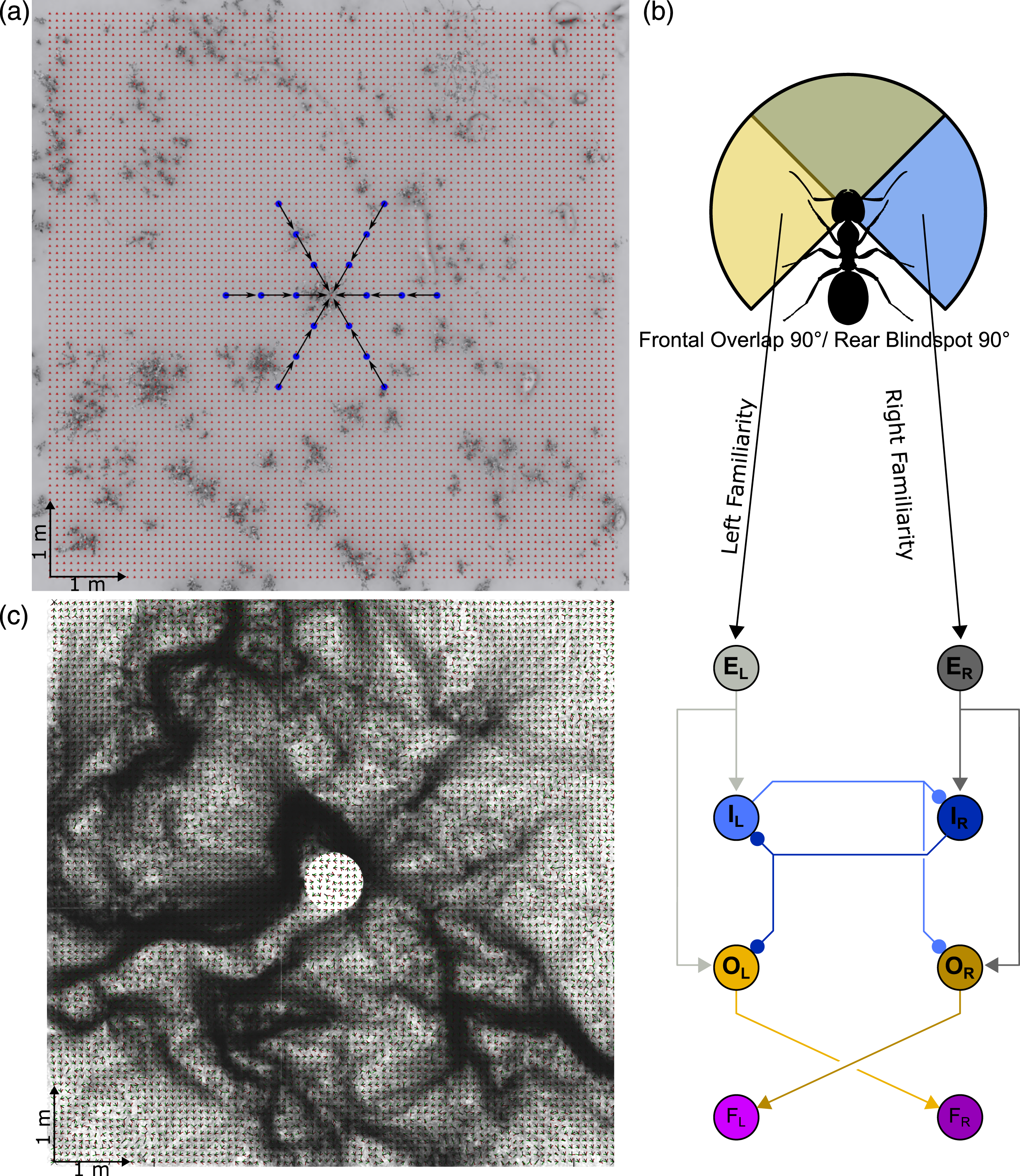

3.6. Summary

Overall, we identified that an Offset is necessary for familiarity taxis to work at all (see Figure 3(a)). Within the range of Offsets we investigated, more than 40° leads to no further improvements (see Figure 3(b)). Increasing fields of view results in more correct steering responses (anything beyond 90° overlap and blindspot, see Figure 3(as)), while decreasing visual resolution does not decrease correct steering responses much (see Figure 4).

4. Discussion

Steering in insects is achieved by an imbalance of activity between left and right descending neurons towards the motor centre (Iwano et al., 2010; Zorovic & Hedwig, 2013). As sensory computation pathways are hemispherically divided, we investigated how two fields of view instead of a single panoramic Field of View can be used so that Snapshot navigation can be implemented via the general steering mode of imabalance activity (Braitenberg, 1984; Steinbeck et al., 2020). To do this, we explored how a difference in familiarity between a left and right Fields of View could achieve a steering response that would keep an agent on a route. We found good performance for large Field of Views and medium to large Offsets. This performance increases with reduced visual resolution and is only slightly affected by aliasing. Therefore, we have shown the plausibility of a steering mechanism based on the inter-hemispheric difference in image familiarity for Snapshot navigation (see Figures 3 and 4).

4.1. Building on pixel-by-pixel comparison

Recent advances in insect neuroscience have inspired other ways in which view-based navigation models can be implemented efficiently. In regard of visual memory, the Mushroom Bodies (MB) have been identified as a structure capable of forming memories of visual stimuli (Buehlmann et al., 2020; Kamhi et al., 2020; Li et al., 2020; Liu et al., 1999; Vogt et al., 2014). A plausible model of how Mushroom Bodies might implement visual memory for navigation comes from Ardin et al. (Ardin et al., 2016). Visual projection neurons connect randomly to a 2nd layer, where each 2nd layer neuron needs activation of multiple inputs to fire. These converge then onto one extrinsic neuron, which introduces a reinforcement signal, therefore associating a certain combination of inputs to a reward. This leads to a measure of familiarity. The number of neurons determine the capacity of this network, scaling the capacity logarithmically. Using this type of memory in a Snapshot model generates comparable performance to other algorithms (Ardin et al., 2016).

For processing of the images we used pixel-by-pixel comparisons, this stage of processing was not intended to be biologically plausible, which made the familiarity processing a simple mathematical operation. This approach can lead to several hurdles though, especially in dynamically changing environments, for example, the same location’s raw pixel value representation may change dramatically with different lighting. To compensate for this, several image processing methods have been proposed. While some methods are similar to feature detection, as with skyline (Graham & Cheng, 2009), landmark (Moeller et al., 1999) or Haar-like features (Baddeley et al., 2011), others take a holistic frequency filtering approach (Meyer et al., 2020; Stone et al., 2018). More computationally intensive methods like object recognition could be employed, albeit probably for simple shapes given low resolution insect vision. Regardless, our approach can be seen to be a minimal demonstration of the recovery of an accurate steering response, any additional ’cognitive’ processes will therefore increase the performance and/or make it more robust to environmental changes. Another filtering approach, which we did investigate, is downsampling of the image size, which effectively acts as a low-pass filter, thereby cancelling out high-frequency noise, as is inherent in the low resolution visual systems of insects (Baddeley et al., 2011; Gerstmayr et al., 2008; Stuerzl & Mallot, 2006). In our analyses, downsampling had a positive effect on performance, as has been shown for visual navigation tasks previously (Milford, 2013; Wystrach et al., 2016a).

In our modelling, visual configurations allowed the independent left and right views, to have a Field of View extending into the contralateral side, i.e. a visual overlap. In insects, we know visual information is transferred to the contralateral hemisphere, it is unclear, however, which visual information is transferred (Habenstein et al., 2020; Li et al., 2020). Therefore, there is a plausible spectrum of no transfer to full transfer of visual information to the contralateral MBs. Indicated by our best performing visual setups (overlap 270° & 360° and 0° blindspot), the more visual information each memory can capture, the better performance. However, it is also true that a FoV using only ipsilateral visual information can be successful too, if in combination with a medium Offset (for example combination 8 with FoV 90°/90°, see Figure 3(a)). A previous investigation of multiple visual fields for Snapshot navigation yielded increased performance with increasing number of visual fields (simulating the hypothetical scenarios of ants having different numbers of compound eyes to cover the whole panorama), with two fields being a plausible trade-off between the number of visual fields of view and the computational effort of determining rIFFs (Wystrach et al., 2016a).

4.2. Visual navigation models

While we mainly focused on investigating how the hemispheric familiarity difference mechanism works when the views from off route locations are compared to the correct memory in the memory sequence, the matching process in an autonomous agent may be less accurate and aliasing may occur, where the most similar memorised snapshot actually originates from a location at another route location (Knight et al., 2020). Aliasing typically reduces performance and comparing each query image to all memorised route snapshots can become computationally expensive, as for this method computation scales linearly with the memorised snapshot number. One attempt to reduce aliasing is inspired by ants’ apparent sequential memory, where they expect certain views to occur one after another (Schwarz et al., 2020). Algorithmically, a temporal window can be introduced, where only a limited amount of the sequentially memorised snapshots is used for familiarity detection. This way, general aliasing can be minimised as well as more complex routes followed (Kagioulis et al., 2021).

Additional robustness of view based navigation might also be gained from different organisations of view memories. For instance, one could be the distinction between attractive and repulsive memories, where the agent would not only memorise snapshots of the direction to move towards (attractive, towards the goal or route direction), but also of the direction not to move towards (repulsive, 180° away from the goal or route direction). This process results in a fine scale sinusoidal movement trajectory (oscillations, (Le Möel & Wystrach, 2020)). While we used an attractive memory, an additional repulsive memory could emphasise a steering response with the attractive memory pulling towards the goal-direction and the repulsive memory pushing away from the anti-goal-direction. Yet another approach could be used to tie the panoramic memories to steering instructions. Whenever heading direction is to the side of the overall goal direction (similar to our offset), that view could be tagged with the appropriate steering direction, where the steering instruction could originate in the LAL (Woodgate et al., 2021; Wystrach et al., 2020).

Our model and that of (Wystrach et al., 2020) differ in the way that steering is determined. Our steering comes from a taxis mechanism driven by visual familiarity difference, whereas (Wystrach et al., 2020) associate turns with specific views, that turn agents back towards the route. This means that the angular offset of stored views is relevant to both models. We also found that an Offset increases a model’s success in steering. This would indicate that snapshots would have to be captured not when an agent’s heading is aligned to route direction, but when the agent’s heading is at an angle. Many ant species oscillate along the route they are following (Clement et al., 2023; Graham & Collett, 2002) which could be part of the strategy of memorising the snapshots with an Offset. We found that the best steering signals are to be found near the Offset of the stored views (Figure 3(c)). Thus for our method and for (Wystrach et al., 2020) oscillations when navigating would come from the agent ’bouncing’ back and forth between leftward and rightward steering. Since the observed oscillations in ants are rather regular however, this could also mean that a source of the oscillations may be internally generated (Clement et al., 2023), perhaps from the LAL (Steinbeck et al., 2020).

We integrated our familiarity-taxis model with our previously LAL-inspired Spiking Neural Network (Steinbeck et al., 2020). Whilst this simulation is not meant to be 100% biologically, and real world, realistic, it does given existence proof that bilateral familiarity fed into LAL inspired SNN model can drive navigational behaviour. Of course, in future, these models can be integrated further with other network models of navigation. Sun et al. (2020) already show a comprehensive architecture for the interaction of navigational modalities (integrating models such as path integration (Stone et al., 2017) and Snapshot navigation (Ardin et al., 2016)) and (Goulard et al., 2020) explore how agents can integrate innate and learned visual programs. As further integration of such models happens with ideas such as more realistic vision and bilateral snapshots (e.g. (Wystrach et al., 2020) and this work) we will be able to make strong predictions for testing in biological experiments. It is already shown that disabling the view of one eye affects the navigational capabilities (Buehlmann, unpublished data, (Schwarz et al., 2023)), as does disabling the memory substrate (MB) of one hemisphere (Buehlmann et al., 2020), further experiments will hopefully exist in a virtuous cycle with computational models.

Footnotes

Declaration of conflicting interests

The author(s) declared no potential conflicts of interest with respect to the research, authorship, and/or publication of this article.

Funding

The author(s) disclosed receipt of the following financial support for the research, authorship, and/or publication of this article: FS was supported by a studentship from the School of Life Sciences, University of Sussex and PG, AOP and TN were supported by EPSRC (Brains on Board project, grant number EP/P006094/1 and activeAI project, grant number EP/S030964/1). TN was also supported by the European Union’s Horizon 2020 research and innovation program under Grant Agreements 785907 (HBP SGA2) and 945539 (HBP SGA3).

ORCID iDs

Fabian Steinbeck

Andrew Philippides

About the Authors

Fabian Steinbeck studied biomimetics and neuroscience before completing a doctorate in neuromimetics at the University of Sussex.

Efstathios Kagioulis is a graduate student studying the application of insect inspired algorithms to robot navigation.

Alex Dewar has a PhD in computational neuroscience and has used modelling and robotic approaches to understanding adaptive behaviour.

Andrew Philippides is a Professor of Biorobotics at the University of Sussex. He has a broad research program in computational biology and AI.

Thomas Nowotny is a Professor in Computational Neuroscience at the University of Sussex. He is an expert in Spiking Neural Networks and GPU and accelerated computation.

Paul Graham is a Professor of Neuroethology an the University of Sussex. He studied for a PhD in neuroscience and has subsequently used behavioural and modelling approaches to study the neural and sensory basis of spatial cognition in insects.

References

Ardin

Peng

Mangan

Lagogiannis

Webb

(2016). Using an insect mushroom body circuit to encode route memory in complex natural environments. PLoS Computational Biology, 12(2), 1–22. https://doi.org/10.1371/journal.pcbi.1004683

Baddeley

Graham

Husbands

Philippides

(2012). A model of ant route navigation driven by scene familiarity. PLoS Computational Biology, 8(1), Article e1002336. https://doi.org/10.1371/journal.pcbi.1002336

Baddeley

Graham

Philippides

Husbands

(2011). Holistic visual encoding of ant-like routes: Navigation without waypoints. Adaptive Behavior, 19(1), 3–15. https://doi.org/10.1177/1059712310395410

Braitenberg

(1984). Vehicles: Experiments in synthetic psychology. MIT Press.

Bresson

Alsayed

Glaser

(2017). Simultaneous localization and mapping: A survey of current trends in autonomous driving. IEEE Transactions on Intelligent Vehicles, 2(3), 194–220. https://doi.org/10.1109/TIV.2017.2749181

Buehlmann

Aussel

Graham

(2020). Dynamic multimodal interactions in navigating wood ants: What do path details tell us about cue integration? Journal of Experimental Biology, 223(7), jeb221036. https://doi.org/10.1242/jeb.221036

Cartwright

B. A.,

Collett

T. S.

(1983). Landmark learning in bees - experiments and models. Journal of Comparative Physiology, 151(4), 521–543. https://doi.org/10.1007/BF00605469

Chahl

J. S.,

Srinivasan

M. V.

(1996). Visual computation of egomotion using an image interpolation technique. Biological Cybernetics, 74(5), 405–411. https://doi.org/10.1007/BF00206707

Chen

Jin

Xia

(2021). Towards a robust visual place recognition in large-scale vSLAM scenarios based on a deep distance learning. Sensors, 21(1), 1–19. https://doi.org/10.3390/s21010310

10.

Clement

Schwarz

Wystrach

(2023). An intrinsic oscillator underlies visual navigation in ants. Current Biology, 33(3), 411–422. https://doi.org/10.1016/j.cub.2022.11.059

11.

Collett

Chittka

Collett

T. S.

(2013). Spatial memory in insect navigation. Current Biology, 23(17), R789–R800. https://doi.org/10.1016/j.cub.2013.07.020

12.

Deneve

Latham

P. E.

Pouget

(2000). Efficient computation and cue integration with noisy population codes. Nature Neuroscience, 4(8), 826–831. https://doi.org/10.1038/90541

13.

Franz

M. O.

(1998). Where did I take that snapshot? Scene-Based homing by image matching. Biological Cybernetics, 79(3), 191–202. https://doi.org/10.1007/s004220050470

14.

Gerstmayr

Röben

Moeller

(2008). From insect visual homing to autonomous robot cleaning. Uni Bielefeld.

15.

Godfrey

R. K.

Swartzlander

Gronenberg

(2021). Allometric analysis of brain cell number in Hymenoptera suggests ant brains diverge from general trends. Proceedings of the Royal Society B: Biological Sciences, 288(1947), 10–17. https://doi.org/10.1098/rspb.2021.0199

16.

Goulard

Buehlmann

Niven

Graham

Webb

(2020). A motion compensation treadmill for untethered wood ants (Formica Rufa): Evidence for transfer of orientation memories from free-walking training. Journal of Experimental Biology, 223(24), jeb228601. https://doi.org/10.1242/jeb.228601

17.

Graham

P.,

Cheng

(2009). Ants use the panoramic skyline as a visual cue during navigation. Current Biology, 19(20), R935–R937. https://doi.org/10.1016/j.cub.2009.08.015

18.

Graham

P.,

Collett

T. S.

(2002). View-based navigation in insects: How wood ants (Formica Rufa L.) look at and are guided by extended landmarks. Journal of Experimental Biology, 205(16), 2499–2509. https://doi.org/10.1242/jeb.205.16.2499

19.

Gridseth

M.,

Barfoot

T. D.

(2021). Keeping an eye on things: Deep learned features for long-term visual localization. IEEE Robotics and Automation Letters, 7(2), 1016–1023. https://doi.org/10.48550/arXiv.2109.04041

20.

Habenstein

Amini

Grübel

el Jundi

Rössler

(2020). The brain of Cataglyphis ants: Neuronal organization and visual projections. Journal of Comparative Neurology, 528(18), 3479–3506. https://doi.org/10.1002/cne.24934

21.

Husbands

Shim

Garvie

Dewar

Domcsek

Graham

Knight

Nowotny

Philippides

(2021). Recent advances in evolutionary and bio-inspired adaptive robotics: Exploiting embodied dynamics. Applied Intelligence, 51(9), 6467–6496. https://doi.org/10.1007/s10489-021-02275-9

22.

Iwano

Hill

E. S.

Mori

Mishima

Ito

Kanzaki

(2010). Neurons associated with the flip-flop activity in the lateral accessory lobe and ventral protocerebrum of the silkworm moth brain. Journal of Comparative Neurology, 518(3), 366–388. https://doi.org/10.1002/cne.22224

23.

Kagioulis

Philippides

Graham

Knight

Nowotny

(2020). Insect inspired view based navigation exploiting temporal information. In Vouloutsi

Mura

Tauber

Speck

Prescott

T. J.

Verschure

P. F. M. J.

(Eds), Biomimetic and biohybrid systems. Living machines 2020. Lecture Notes in Computer Science (vol. 12413). Springer.

24.

Kagioulis

Philippides

Graham

Knight

J. C.

Nowotny

(2021). Insect inspired view based navigation exploiting temporal information. In Lecture Notes in Computer Science(including subseries Lecture Notes in Artificial Intelligence and Lecture Notes in Bioinformatics), 12413 LNAI, 204216. Springer

25.

Kamhi

Barron

Narendra

(2020). Vertical lobes of the Mushroom Bodies are essential for view-based navigation in Australian Myrmecia Ants. Current Biology, 30(17), 3432. https://doi.org/10.1016/j.cub.2020.06.030

26.

Kanzaki

Sugi

Shibuya

(1992). Self-generated zigzag turning of Bombyx-Mori males during pheromone-mediated upwind walking. Zoological Science, 9(3), 515–527. https://doi.org/10.34425/zs000983

27.

Knight

J. C.

Sakhapov

Domcsek

Dewar

A. D.

Graham

Nowotny

Philippides

(2020). Insect-inspired visual navigation on-board an autonomous robot: Real-world routes encoded in a single layer network. In Proceedings of the 2019 conference on artificial Life: How can artificial Life help solve societal challenges (pp. 60–67). ALIFE 2019.

28.

Kodzhabashev

Mangan

(2015). Route following without scanning. Lecture Notes in Computer Science, 9222(Proceedings 4), 199–210. https://doi.org/10.1007/978-3-319-22979-9_20

29.

Labrosse

(2006). The visual compass: Performance and limitations of an appearance-based method. Journal of Field Robotics, 23(10), 913–941. https://doi.org/10.1002/rob.20159

30.

Le Möel

F.,

Wystrach

(2020). Opponent processes in visual memories: A model of attraction and repulsion in navigating insects’ mushroom bodies. PLoS Computational Biology, 16(2), 1–24. https://doi.org/10.1371/journal.pcbi.1007631

31.

Lent

D. D.

Graham

Collett

T. S.

(2010). Image-matching during ant navigation occurs through saccade-like body turns controlled by learned visual features. Proceedings of the National Academy of Sciences of the United States of America, 107(37), 16348–16353. https://doi.org/10.1073/pnas.1006021107

32.

Mahoney

B. D.

Jacob

M. S.

Caron

S. J. C.

(2020). Visual input into the Drosophila melanogaster mushroom body. Cell Reports, 32(11), 108138. https://doi.org/10.1016/j.celrep.2020.108138

33.

Liu

Wolf

Ernst

Heisenberg

(1999). Context generalization in Drosophila visual learning requires the mushroom bodies. Nature, 400(6746), 753–756. https://doi.org/10.1101/lm.318606

34.

Meyer

Nowotny

Graham

Dewar

A. D.

Philippides

(2020). Snapshot Navigation in the wavelet domain. In Living machines 2020: Biomimetic and biohybrid systems (pp. 245–256). Springer.

35.

Milford

(2013). Vision-based place recognition: How low can you go? The International Journal of Robotics Research, 32(7), 766–789. https://doi.org/10.1177/0278364913490323

36.

Moeller

(2012). A model of ant navigation based on visual prediction. Journal of Theoretical Biology, 305, 118–130. https://doi.org/10.1016/j.jtbi.2012.04.022

37.

Moeller

Maris

Lambrinos

(1999). A neural model of landmark navigation in insects. Neurocomputing, 26-27(26), 801–808. https://doi.org/10.1016/S0925-2312(98)00150-7

38.

Moeller

R.,

Vardy

(2006). Local visual homing by matched-filter descent in image distances. Biological Cybernetics, 95(5), 413–430. https://doi.org/10.1007/s00422-006-0095-3

39.

Namiki

Iwabuchi

Pansopha Kono

Kanzaki

(2014). Information flow through neural circuits for pheromone orientation. Nature Communications, 5(5), 5919. https://doi.org/10.1038/ncomms6919

40.

Namiki

Kanzaki

(2016). The neurobiological basis of orientation in insects: Insights from the silkmoth mating dance. Current Opinion in Insect Science, 15(7), 16–26. https://doi.org/10.1016/j.cois.2016.02.009

41.

Narendra

(2007). Homing strategies of the Australian desert ant Melophorus bagoti II. Interaction of the path integrator with visual cue information. Journal of Experimental Biology, 210(10), 1804–1812. https://doi.org/10.1242/jeb.02769

42.

Pansopha

Ando

Kanzaki

(2014). Dynamic use of optic flow during pheromone tracking by the male silkmoth, Bombyx mori. Journal of Experimental Biology, 217(10), 1811–1820. https://doi.org/10.1242/jeb.090266

43.

Paulk

A. C.

Kirszenblat

Zhou

van Swinderen

(2015). Closed-loop behavioral control increases coherence in the fly brain. Journal of Neuroscience, 35(28), 10304–10315.

44.

Philippides

Baddeley

Cheng

Graham

(2011). How might ants use panoramic views for route navigation? Journal of Experimental Biology, 214(3), 445–451. https://doi.org/10.1242/jeb.046755

45.

Philippides

de Ibarra

Riabinina

Collett

(2013). Bumblebee calligraphy: The design and control of flight motifs in the learning and return flights of bombus terrestris. Journal of Experimental Biology, 216(6), 1093. https://doi.org/10.1242/jeb.081455

46.

Rayshubskiy

Holtz

D’Alessandro

Vanderbeck

Haber

Gibb

Wilson

(2020). Neural control of steering in walking Drosophila. Harvard University.

47.

Risse

Mangan

Stuerzl

Webb

(2018). Software to convert terrestrial LiDAR scans of natural environments into photorealistic meshes. Environmental Modelling & Software, 99(99), 88–100. https://doi.org/10.1016/j.envsoft.2017.09.018

48.

Schwarz

Clement

Haalck

Risse

Wystrach

(2023). Compensation to visual impairments and behavioral plasticity in navigating ants. bioRxiv.

49.

Schwarz

Mangan

Webb

Wystrach

(2020). Route-following ants respond to alterations of the view sequence. Journal of Experimental Biology, 223(14), 218701. https://doi.org/10.1242/jeb.218701

50.

Schwarz

Mangan

Zeil

Webb

Wystrach

(2017). How ants use vision when homing backward. Current Biology, 27(3), 401–407. https://doi.org/10.1016/j.cub.2016.12.019

51.

Schwarz

Narendra

Zeil

(2011). The properties of the visual system in the Australian desert ant Melophorus bagoti. Arthropod Structure & Development, 40(2), 128–134. https://doi.org/10.1016/j.asd.2010.10.003

52.

Smith

Philippides

Graham

Baddeley

Husbands

(2007). Linked local navigation for visual route guidance. Adaptive Behavior, 15(3), 257–271. https://doi.org/10.1177/1059712307082091

53.

Smith

R. C.,

Cheeseman

(1986). On the representation and estimation of spatial uncertainty. The International Journal of Robotics Research, 5(4), 56–68. https://doi.org/10.1177/027836498600500404

54.

Steinbeck

Adden

Graham

(2020). Connecting brain to behaviour: A role for general purpose steering circuits in insect orientation? Journal of Experimental Biology, 223(4), jeb212332. https://doi.org/10.1242/jeb.212332

55.

Steinbeck

Nowotny

Philippides

Graham

(2022). Production of adaptive movement patterns via an insect inspired spiking neural network central pattern generator. bioRxiv. https://doi.org/10.1101/2022.04.07.487574

56.

Stone

Mangan

Wystrach

Webb

(2018). Rotation invariant visual processing for spatial memory in insects. Interface Focus, 8(4), 20180010. https://doi.org/10.1098/rsfs.2018.0010

57.

Stone

Webb

Adden

Weddig

N. B.

Honkanen

Templin

Wcislo

Scimeca

Warrant

Heinze

(2017). An anatomically constrained model for path integration in the Bee brain. Current Biology, 27(20), 3069–3085.e11. https://doi.org/10.1016/j.cub.2017.08.052

58.

Stuerzl

Cheung

Cheng

Zeil

(2008). The information content of panoramic images I: The rotational errors and the similarity of views in rectangular experimental arenas. Journal of Experimental Psychology: Animal Behavior Processes, 34(1), 1–14. https://doi.org/10.1037/0097-7403.34.1.1

59.

Stuerzl

W.,

Mallot

H. A.

(2006). Efficient visual homing based on Fourier transformed panoramic images. Robotics and Autonomous Systems, 54(4), 300–313. https://doi.org/10.1016/j.robot.2005.12.001

60.

Sun

Yue

Mangan

(2020). A decentralised neural model explaining optimal integration of navigational strategies in insects. Elife, 9(9), 1–30. https://doi.org/10.7554/eLife.54026

61.

Vogt

Schnaitmann

Dylla

K. V.

Knapek

Aso

Rubin

G. M.

Tanimoto

(2014). Shared mushroom body circuits underlie visual and olfactory memories in Drosophila. Elife, 3(3), e02395. https://doi.org/10.7554/eLife.02395#.dpuf

62.

Wang

Bovnik

Sheikh

Simoncelli

(2004). Image quality assessment: From error visibility to structural similarity. IEEE Transactions on Image Processing, 13(4), 600–612. https://doi.org/10.1109/TIP.2003.819861

63.

Woodgate

Perl

Collett

(2021). The routes of one-eyed ants suggest a revised model of normal route following. Journal of Experimental Biology, 224(16), jeb242167. https://doi.org/10.1242/jeb.242167

64.

Wystrach

Dewar

Philippides

Graham

(2016a). How do field of view and resolution affect the information content of panoramic scenes for visual navigation? A computational investigation. Journal of Comparative Physiology: Neuroethology, Sensory, Neural, and Behavioral Physiology, 202(2), 87–95. https://doi.org/10.1007/s00359-015-1052-1

65.

Wystrach

Le Moël

Clement

Schwarz

(2020). A lateralised design for the interaction of visual memories and heading representations in navigating ants. bioRxiv, 5(5). https://doi.org/10.1101/2020.08.13.249193

66.

Wystrach

Mangan

Philippides

Graham

(2013). Snapshots in ants? New interpretations of paradigmatic experiments. Journal of Experimental Biology, 216(10), 1766–1770. https://doi.org/10.1242/jeb.082941

67.

Wystrach

Philippides

Aurejac

Cheng

Graham

(2014). Visual scanning behaviours and their role in the navigation of the Australian desert ant Melophorus bagoti. Journal of Comparative Physiology: Neuroethology, Sensory, Neural, and Behavioral Physiology, 200(7), 615–626. https://doi.org/10.1007/s00359-014-0900-8

68.

Zeil

(2012). Visual homing: An insect perspective. Current Opinion in Neurobiology, 22(2), 285–293. https://doi.org/10.1016/j.conb.2011.12.008

69.

Zeil

Hofmann

M. I.

Chahl

J. S.

(2003). Catchment areas of panoramic snapshots in outdoor scenes. Journal of the Optical Society of America A, 20(3), 450. https://doi.org/10.1364/josaa.20.000450

70.

Zorovic

M.,

Hedwig

(2013). Descending brain neurons in the cricket Gryllus bimaculatus (de Geer): Auditory responses and impact on walking. Journal of Comparative Physiology A: Neuroethology, Sensory, Neural, and Behavioral Physiology, 199(1), 25–34. https://doi.org/10.1007/s00359-012-0765-7

Familiarity-taxis: A bilateral approach to view-based snapshot navigation

Abstract

Keywords

1. Introduction

2. Methods

2.1. Antworld image rendering

2.2. Field of view

2.3. Offset

2.4. Image processing

2.5. Rotary Image Familiarity Function

2.6. Measures of successful steering

2.7. Evaluation of aliasing

3. Results

3.1. Overall performance of a bilateral visual familiarity method

3.2. Organisation of visual system

3.3. Visual resolution

3.4. Aliasing

3.5. Central place navigation task

3.6. Summary

4. Discussion

4.1. Building on pixel-by-pixel comparison

4.2. Visual navigation models

Footnotes

Declaration of conflicting interests

Funding

ORCID iDs

About the Authors

References