Sage Journals: Discover world-class research

Abstract

This article presents a scenario where a simple simulated organism must explore and exploit an environment containing a food pile. The organism learns to make observations of the environment, use memory to record those observations, and thus plan and navigate to the regions with the strongest food density. We compare different reinforcement learning algorithms with an adaptive dynamic programming algorithm and conclude that backpropagation through time can convincingly solve this recurrent neural-network challenge. Furthermore, we argue that this algorithm successfully mimics a minimal ‘functionally sentient’ organism’s fundamental objectives and mental environmental-mapping skills while seeking a food pile distributed statically or randomly in an environment.

Keywords

Back propagation through time BPTT adaptive behaviour ADP algorithm control task partially observable environment

Introduction

Existing Reinforcement Learning (RL) and Adaptive Dynamic Programming (ADP) algorithms have become more efficient in examining, learning and solving new problems (e.g., a new game) (Mnih et al., 2013; Silver et al., 2018). However, solutions can be computationally demanding as the algorithms slowly adapt to a new problem. The existing RL methods cannot efficiently adapt to an existing problem that has been learnt once but then changes its rules (Li et al., 2018). This article presents a surprisingly simple partial-observability problem where the goal is randomised, and many ADP/RL algorithms struggle to solve it.

A partially observable domain is one in which the agent does not receive inputs describing the whole state of the system at once. Consequently, an ‘observation sequence’ is required for the agent to recreate the ‘state’ from observations (in the form of a belief model, a predictive state representation, or any other scheme). Intuitively, a partially observable domain is analogous to a poker game; one needs to observe sequences of opponent actions to try and recreate the state. A simple ‘bird’s-eye’ look at the table is not enough.

We propose a close-to-minimal problem in a partially observable environment, where an agent has to use observations and its internal memory to learn to navigate and move towards a randomly positioned food source – see Figure 1. The food source’s location is randomised at every ‘game’ reset, where the agent is re-initialised according to its original position. The agent receives sensory data of the density of food at its current location (this is the height of the Gaussian bump, i.e. a single scalar reading) at every time step of its journey.

Figure 1.

Simple food density distribution, where the height of the Gaussian bump indicates food density. Pathway shows an example solution trajectory found by the agent, starting at the bottom and finishing at the ‘x’.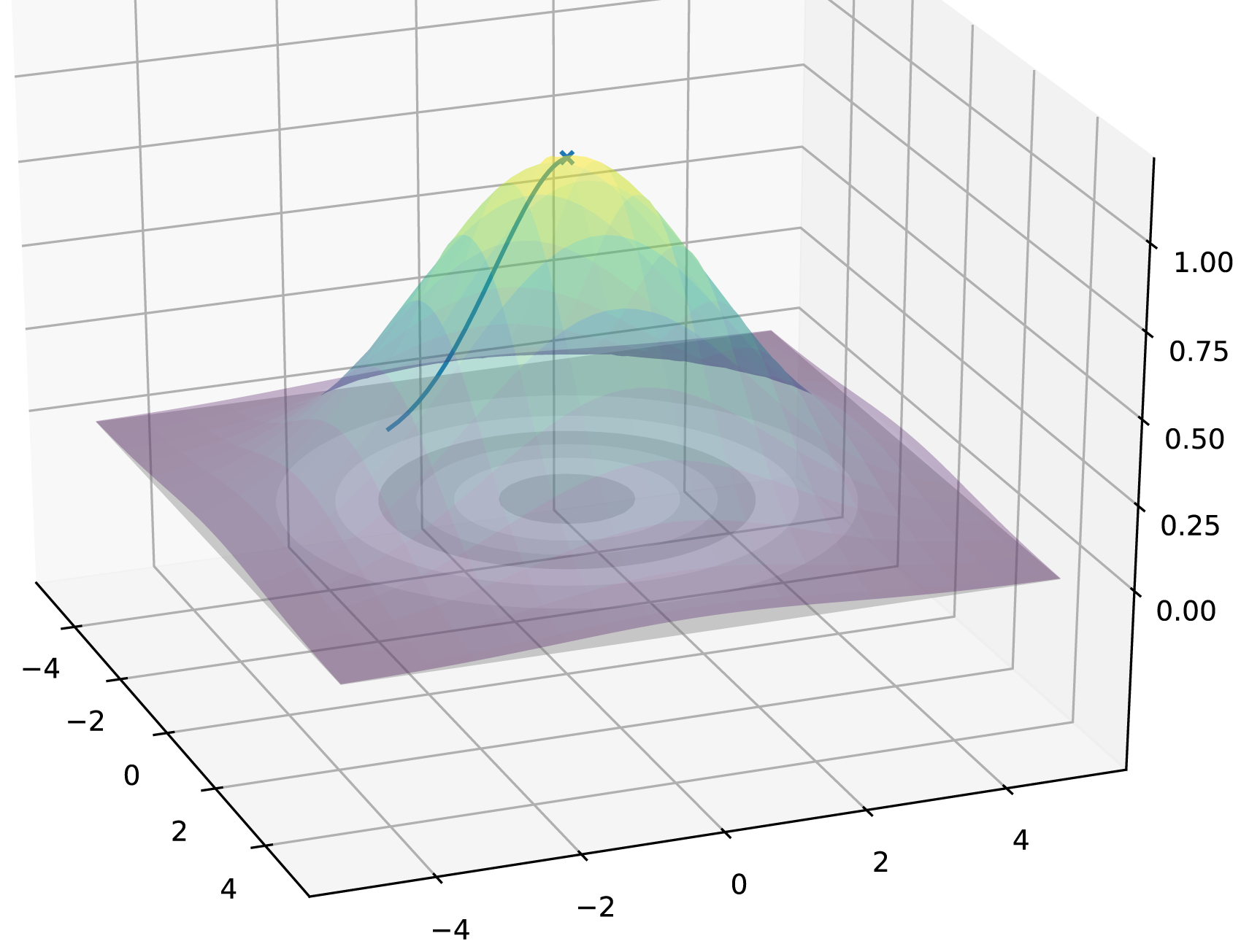

To solve the proposed problem:

• The agent has to devise a movement strategy that quickly explores, taking samples of the food density at multiple nearby locations.

• It also must devise a memory strategy that quickly records observations to acquire the location information about the food source. Then, an exploitation strategy quickly moves the agent towards the discovered densest food location.

This solution requires a recurrent neural network (RNN) with recurrent-memory nodes to act as an exploration and memorisation strategy. It also requires an ADP/RL algorithm to discover this RNN exploration algorithm.

It is known that RNNs are of importance in understanding the brain (Prince et al., 2021). It also is known that RNNs are, in theory, Turing Complete (Chung and Siegelmann 2021), and therefore, each point of an RNN’s weight-space potentially represents a different possible algorithm. Therefore, if the RNN architecture is sufficiently large, there should be at least one point in weight-space representing an RNN algorithm capable of solving the food-exploration problem we are setting it.

The RNN algorithm will require the formation of memories about the partially explored environment and goal. Hence, the RNN algorithm must be capable of learning about its environment. It is the objective of the ADP/RL algorithm to find such a set of weights. If the ADP/RL algorithm manages this, it must have ‘learned how to learn’ or performed meta-learning.

Hence, there are two levels of learning required here: the inner learning algorithm executed by the RNN as it explores the food environment; and the outer learning algorithm, that is, the ADP/RL algorithm, which discovers an RNN exploration algorithm capable of doing this.

Even though this food-exploration challenge is relatively easy and could easily be solved by many pre-existing hill-climbing algorithms from computer science, the RNN algorithm we seek must be discovered by the ADP/RL algorithm instead of being hand-programmed. Furthermore, the RNN algorithm must be self-adaptive to any new randomised location for the food pile without requiring further tuning of its weights.

To tackle this partially observable environment, we selected all RL algorithms applicable to continuous action and state spaces, which were readily available in the current version of the Stable-Baselines package (Raffin et al., 2019) (version 1.1.0). These included Advantage Actor-Critic (A2C), Soft Actor-Critic (SAC), Deep Deterministic Policy Gradient (DDPG) and Twin Delayed DDPG (TD3) (Mnih et al., 2016; Haarnoja et al., 2017; Lillicrap et al., 2015; Fujimoto et al., 2018). We also used the classic ADP model-based algorithm, backpropagation through time (BPTT, Werbos (1990); Lillicrap and Santoro (2019)). However, our experiments show that the selected state-of-the-art RL algorithms could not devise a policy that causes the agent to devise such a recurrent-memory–based exploration strategy.

Contrarily, our implemented BPTT devised an exploration strategy with recurrent-memory features. This outcome is consistent with prior work by Fairbank, Li, et al. (2014), which shows that BPTT is capable of finding RNN solutions for exploiting partially observable environments, and also that BPTT can exhibit more robust convergence than classic RL algorithms (Fairbank et al., 2013). Although it can be argued that BPTT is not a ‘true’ RL algorithm since it requires access to a known environment model, we show that using BPTT to train the agent uniquely enables a solution to be found. Moreover, BPTT’s advantage of receiving model-based gradient information about the environment is crucial in solving this task.

We propose that this navigational problem, and the RNN’s algorithm that must be learned to solve it, emulate in the simplest possible sense, the memory-manipulation tasks that some organisms must perform to locate foods (e.g. E-coli bacteria sensory-based navigation (Hu and Tu 2014)). Hence, we argue that this RNN is functionally equivalent to the food-seeking sentient behaviour of the simplest organisms. It includes the formation of memories that describe the agent’s environment and the goal-directed adaptive behaviour to exploit the environment and obtain food. By ‘functionally sentient’, we mean that the external behaviours of the agent mimic those of a sentient creature. We do not make any claims as to whether our simulation is sentient or such simple organisms are. Our approach follows a long tradition in adaptive-behaviour research of developing ‘minimal agents’ (Conway et al., 1970; Braitenberg, 1986; Beer, 2003) that portray complicated behaviour.

One of the critical challenges for the agent in this particular task is that the single environment sensor returns only one scalar value. Hence, to deduce the slope of the food gradient, several scalar readings are required (i.e. requiring a memory), and these must be combined by some sort of algorithm (e.g. triangulation) to deduce the food density gradient. While this might require some thought for a human programmer to devise a solution algorithm, this all needs self-learning by an RNN. Moreover, once solved, there are some capabilities of the RNN which are common to simple organisms which are assumed sentient:

1. It has an internal belief state about its environment (e.g. current estimation of food gradient? What was the agent’s previous location?).

2. This belief state of its environment changes as it explores.

3. It must execute a purposeful movement strategy to increase knowledge (exploration).

4. It must perform some form of computation on its memories (e.g. triangulation) to fully exploit the environment.

5. Once the goal is discovered, it moves towards it (exploitation).

We show that the two significant challenges of a partially observable environment and unexpected perturbations to the environment (Braun et al., 2009) have been simulated and solved in our experiments. The unexpected perturbations consisted of randomising the food location at every environment reset. We implemented a simplified form of the gated recurrent unit (GRU; Chung et al. (2014)), working with sensors to tackle this problem and overcome these challenges.

This article contributes to current knowledge by emphasising the usefulness of BPTT in simple biologically feasible exploration contexts, where some form of memory manipulation and algorithmic discovery is required for their solution. Although it is a classic 1990 algorithm (Werbos, 1990), BPTT is often overlooked in reinforcement learning, yet here we show it can outperform some state-of-the-art reinforcement learning algorithms. We have also shown how a simplified GRU memory can be incorporated into this navigational algorithmic-discovery task.

The rest of the article is structured as follows: The Related Work section describes other ADP/RL work that tackles partially observable domains, plus meta-learning and ‘learning to learn’. Next, the Environment and Agent Definitions section describes the physics world that the agent explores, the sensing capabilities of the agent, and the memory model it uses. The Backpropagation Through Time Algorithm section describes how BPTT is not just restricted to learning static time sequences, but can also be used to train an agent in this ADP/RL setting. The Experiments section compares the various ADP/RL algorithms’ abilities to solve two versions of the problem – a simplified problem that is fully observable and the main partially observable problem. Next, the Discussion section compares the BPTT performance with the selected state-of-the-art algorithms in tackling the partially observable environment and attempts to account for the differences. Finally, the Conclusion section summarises our findings and explains future work needing to be done.

Related Work

This section describes related research to tackle partially observable domains using ADP/RL algorithms. Different approaches to achieving meta-learning are compared, and their identification as meta-learning is observed.

Tackling Partially Observable Environments

Partially Observable Markov Decision Processes (POMDPs) (Kaelbling et al., 1998) can be used to tackle domains where they map the history of observations to actions. One of the most effective ways to train POMDP policies is through Recurrent Neural Networks (RNNs) (Wierstra et al., 2007; 2010). As stated by Wierstra et al. (2010), traditional approaches such as value-function methods applied to RNNs had sub-par performance when given incomplete state observations. Therefore, Wierstra et al. (2010) introduced the Recurrent Policy Gradient (RPG) algorithm to learn memory-based policies for deep-mapping memory POMDPs. This algorithm back-propagates the estimated return-weighted ‘eligibilities’ backwards through time using an RNN. Wierstra et al. (2010) showed that policy updates could become a function of any event in the recorded history, using the backpropagation through time method. This approach outperformed other state-of-the-art RL algorithms in three important game-like benchmarks.

Similarly to Wierstra et al. (2010), Hausknecht and Stone (2015) observed that standard value-based methods had considerable room for improvement when dealing with POMDPs. Their proposed solution was to modify a Deep Q-Network (DQN) to deal with POMDPs. Their approach was named Deep Recurrent Q-Network (DRQN) and combined Long Short Term Memory (LSTM) (Hochreiter and Schmidhuber 1997) with a DQN. They experimented with flickering Atari domains – a modification to the classic Atari games such that the agent is given either fully revealed or fully obscured observation with probability p = 0.5. They trained models with full observations and evaluated them with partial observations. They argued that the flickering rate in these domains directly affected the performance of the DQN. However, over a range of 10 different games where flickering was used, they found that using an RNN only improved the agent’s performance in one of those 10 games.

In other testing domains, Wierstra et al. (2010) showed that recurrency could be a helpful method for handling state observations. However, they showed that stacking the observations in the input layer of a convolutional network performs similarly to the recurrency method used by Hausknecht and Stone (2015) in their chosen domains; this can be seen as a way to turn the POMDP problem into a finite-memory MDP (Kaelbling et al., 1998). A controller on n previous observations can be as successful as a recurrent neural network’s internal ‘belief’ state if this is all that environment dynamics needs.

Meta-Learning

Meta-learning, a former informal notion of cognitive psychology that is also referred to as ‘learning to learn’, was more recently developed into a formal notion of machine learning (Schaul and Schmidhuber 2010). Schaul and Schmidhuber (2010) define meta-learning as the process of learning how to learn in the context of machine learning. Informally, a meta-learning algorithm alters a learning algorithm or the learning process based on experience. The updated learner is more adept at gaining knowledge from new experiences than the original learner.

Meta-learning is approached differently by different researchers. In a setup where a series of different tasks with a shared underlying set of regularities, Thrun and Pratt (1998) state that the rapid improvement of the agent’s performance in each new task can be identified as meta-learning. At the architectural level, meta-learning is conceptualised as involving two learning systems: a lower-level (or ‘inner’) system which learns quickly and is primarily responsible for adapting to each new task; and a higher-level (or ‘outer’) system which learns more slowly and works across tasks to improve the lower-level system (Prokhorov et al., 2002; Younger et al., 2001).

Some researchers interpret meta-learning in a much stronger sense, requiring it specifically to mean being able to replicate the adaptive weight processes which occur when training neural networks. For example, Cotter and Conwell (1990)’s early work showed how fixed-weight RNNs could approximate an adaptive-weight learning algorithm. They demonstrated this idea by transforming a backward error propagation network into a fixed-weight system. Younger et al. (1999) expanded upon this idea by using an RNN to store knowledge analogous to short-term memory. This method allowed the neural network to learn dynamically, enabling learning to occur continually as part of the net’s behaviour.

Younger et al. (2001) and Prokhorov et al. (2002) used the term meta-learning to describe adaptive behaviour with fixed weights in RNNs. However, Lo and Bassu (2001) used alternative terminology by referring to fixed-weight adaptive RNN behaviour as ‘accommodative’ neural networks. In this article, we use the term meta-learning as used by Younger et al. (2001) and Prokhorov et al. (2002).

Similarly to Thrun and Pratt (1998), Hochreiter et al. (2001) presented an RNN that was trained on a series of interrelated tasks using standard backpropagation, where the network received an auxiliary input indicating the target output for the preceding step. Compared with Prokhorov et al. (2002), Hochreiter et al. (2001) focus on the knowledge-transfer mechanism using RNNs. They argued that using an RNN to represent a differentiable version of a Turing machine was possible. Furthermore, they hypothesised that gradient-based optimisation approaches could derive a learning algorithm from a random starting point.

Santoro et al. (2016) suggested that augmented-memory neural networks (MANNs) can perform meta-learning in tasks that require short- and long-term memory. To obtain useful representations of raw data (meta-representation), they used gradient descent to learn an abstract method slowly. In addition, they incorporated an external memory module to bind never-before-seen information rapidly. Their method was based on Neural Turing Machines (Graves et al., 2014), architectures with augmented memory capacities. These architectures offer the ability to encode and retrieve new information quickly.

The previously mentioned works on meta-learning (i.e. by Cotter and Conwell (1990), Younger et al. (1999), Hochreiter et al. (2001), Prokhorov et al. (2002) and Santoro et al. (2016)) only addressed their algorithm’s usage in supervised learning. However, our article will demonstrate meta-learning in a control problem where the environment is partially observable.

One of the recent popular approaches to meta-learning in RL (known as ‘meta reinforcement learning’) is made by Finn et al. (2017); Nichol and Schulman (2018) suggesting a method at the validation time to learn an initialisation of the model-agnostic meta-learning (MAML) model. Finn et al. (2017) showed that MAML learns a model that can quickly adapt with a single gradient update which resulted in a few gradient steps to achieve a good performance. However, the methods provided by Finn et al. (2017) and Nichol and Schulman (2018) do not explicitly consider the necessity of exploring the initial policy. This problem is addressed by Stadie et al. (2018), where they considered per-task sampling distributions as extra information for exploration; exploration for model-agnostic meta-learning (E-MAML) typically consists of a feed-forward policy. This method optimises the per-task sample distributions about the anticipated future returns generated by the post-adaptation policy explicitly during adaptation.

Ortega et al. (2019) proposed a method to recast memory-based meta-learning within a Bayesian framework; this memory-based meta-learning translates the hard problem of probabilistic sequential inference into a regression problem. According to Ortega et al. (2019), this is accomplished by amortising data that has been Bayes-filtered, with the adaptation being implemented in the memory dynamics as a state-machine with adequate statistics.

Adaptive Dynamic Programming

Adaptive Dynamic Programming (ADP) (Murray et al., 2002; Wang et al., 2009; Prokhorov and Wunsch 1997) and Reinforcement Learning (RL) (Sutton and Barto 2018) are closely related; both aim to learn a policy function that maximises a long-term reward function. However, a critical difference between ADP and RL is that ADP is not restricted to assuming that the environment is a black box. This allows ADP to take advantage of efficient gradient calculations through the environment. Prominent ADP methods which do this are BPTT and its critic-based relative Dual Heuristic Programming (DHP) (Prokhorov and Wunsch 1997; Fairbank et al., 2012, 2014b). These are appropriate when the state space is continuous and the environment’s physics model is known and differentiable. Under these circumstances, DHP and BPTT can learn much more quickly than model-free RL models, sometimes quicker by several orders of magnitude (Fairbank and Alonso 2012).

Fu et al. (2014) enhanced training an RNN with BPTT, by using the Levenberg-Marquardt (LM) algorithm as an accelerated optimiser. The algorithm was tested to control a grid-connected converter (GCC) optimally. The results presented by Fu et al. (2014) showed the combination of the LM algorithm and a forward accumulation through time (FATT) to calculate the Jacobian matrix could train RNNs better than the BPTT algorithm without LM.

However, despite BPTT’s reliance on its knowledge of a physics model, BPTT can allow an agent to be adaptive when an environment’s physics model is changing (Fairbank, Li, et al., 2014). Fairbank, Li, et al. (2014) give another example of such adaptive behaviour through model-based differentiable physics models of the environment.

Fairbank and Alonso (2012) presented a different minimal setup where the ADP algorithm outperformed model-free algorithms. Fairbank, Li, et al. (2014) show how BPTT can train an adaptive agent in an electrical control task. We extend these works here by training an RNN to perform a memory-manipulation task in a more biologically relevant environment.

Teichmann (2015) used ADP/RL methods to train simulated agents foraging for food in an environment. Their work differs from ours in that it only handled static food distributions. Hence the agent’s (x, y) coordinates indicate the food density, and Teichmann (2015)’s work did not need to use meta-learning to create an algorithm capable of seeking out a randomised food location.

Environment and Agent Definitions

We developed an environment to test navigational tasks. The agent (a simulated organism) has the task of finding the densest point of a food pile in this environment.

Environment Rewards

A two-dimensional environment was created for an agent to explore and navigate. In the environment, there is a food pile parameterised by (x_food, y_food, z_food, σ_food). The following Gaussian-type function describes the food-pile’s density at location (x, y)

d (x, y) = z_{food} + \exp (\frac{{(x - x_{food})}^{2} + {(y - y_{food})}^{2}}{σ_{food}^{2}})

(1)

Here z_food is a constant specifying the food-pile height, and σ_food is a parameter governing the width of the food bump. For example, see Figure 1.

As the agent moves across the environment at discrete time step t, it has location (x_t, y_t), and it uptakes the food at its new position (x_t, y_t). The food supply at any location is deemed inexhaustible. Hence, the total food accumulated during an episode of length L steps is given by

R = \sum_{t = 0}^{L - 1} γ^{t} r_{t}

(2)

where r_t = d (x_t, y_t) and 0 ≤ γ ≤ 1 is a discount factor.

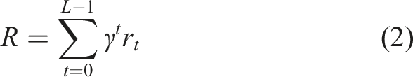
The objective of our problem is for the agent to learn to rapidly walk to the top of the food pile to maximise the food (reward) accumulated in a fixed finite episode length L = 30. Furthermore, the location and height of the food pile are randomised; this forces the agent to make observations and use memory to maximise the reward in any episode.

Agent’s Physics

In the simple case with no memory, at each time step t, the agent outputs a two-dimensional action vector ${\vec{a}}_{t} \in R^{2}$ . The velocity ${\vec{v}}_{t}$ of the agent is determined by

{\vec{v}}_{t} = v_{\max} \tanh (| {\vec{a}}_{t} |) {\hat{a}}_{t}

(3a)

where

| {\vec{a}}_{t} |

is the Euclidean length,

{\hat{a}}_{t} = {\vec{a}}_{t} / | {\vec{a}}_{t} | + ϵ

, ϵ = 10⁻⁶ and v_max = 0.2. The tanh appearing in (3a) limits the agent’s speed to less than v_max. The construction of (3a) allows the velocity vector

{\vec{v}}_{t}

to be anywhere strictly inside a circle of radius v_max. This will allow the agent to wander freely in any direction. The position of the agent is updated according to the velocity vector

{\vec{v}}_{t}

, using the Euler method with a discrete time step ΔT = 1

\begin{array}{l} {\vec{p}}_{t + 1} = {\vec{p}}_{t} + {\vec{v}}_{t} Δ T, \end{array}

(3b)

where

{\vec{p}}_{t} = (x_{t}, y_{t})

is the agent’s position at the specified time step.

Agent Brain

A neural network with weight vector $\vec{w}$ chooses the actions and memory state of the agent. We refer to this neural network as the ‘agent brain’; but this neural network is also known as the ‘actor’ in the RL literature, or the ‘action network’ in the ADP literature.

At any time step t, the agent receives an observation vector ${\vec{o}}_{t}$

{\vec{o}}_{t} = (x_{t}, y_{t}, d (x_{t}, y_{t}))

(4)

The final component of ${\vec{o}}_{t}$ represents a scalar sensor reading that the agent receives about the food density at their current location, given by (1). In some experiments, we omitted this sensor reading from the observation vector ${\vec{o}}_{t}$ .

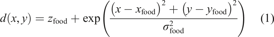
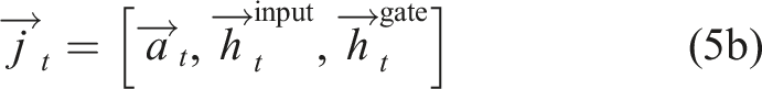
The memory state of the agent at time t is given by a vector ${\vec{h}}_{t} \in R^{m}$ , where m is the number of recurrent-memory nodes.

The neural network we implemented is shown in Figure 2. It has $\dim ({\vec{o}}_{t}) + m$ inputs and $\dim ({\vec{a}}_{t}) + 2 m$ output nodes. This allows for recurrence in the neural network and allows the neural network to receive observations $({\vec{o}}_{t})$ as input and to make a control action $({\vec{a}}_{t})$ as output. At time t, the output vector ${\vec{j}}_{t}$ of the neural network is given by

{\vec{j}}_{t} = π ({\vec{h}}_{t}, {\vec{o}}_{t}, \vec{w})

(5a)

where π denotes the neural network,

{\vec{o}}_{t}

is the observation vector at time t and

{\vec{h}}_{t}

is the recurrent-memory state at time t.

Figure 2.

Main neural-network structure used in our experiments.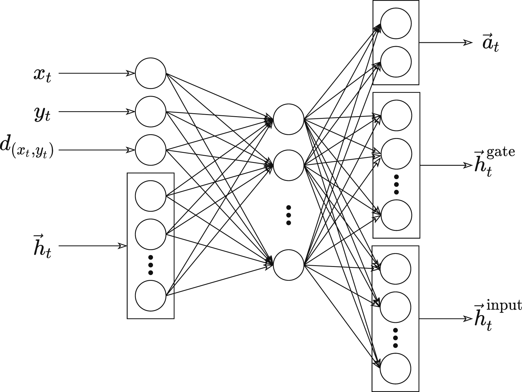

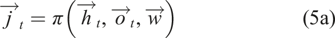
The output vector ${\vec{j}}_{t}$ is partitioned into chunks defined by

{\vec{j}}_{t} = [{\vec{a}}_{t}, {\vec{h}}_{t}^{input}, {\vec{h}}_{t}^{gate}]

(5b)

as shown in Figure 2.

Here, ${\vec{a}}_{t}$ is the action vector (of length 2) chosen by the agent in this deterministic policy function, and ${\vec{h}}_{t}^{input}$ and ${\vec{h}}_{t}^{gate}$ (each of length m) are memory gates and inputs, which are used to provide a GRU-style recurrent memory.

The recurrent memory is updated during each time step by the equation

{\vec{h}}_{t + 1} = \tanh ({\vec{h}}_{t}^{input}) ʘ σ ({\vec{h}}_{t}^{gate}) + {\vec{h}}_{t} ʘ (1 - σ ({\vec{h}}_{t}^{gate}))

(6)

where σ denotes the logistic sigmoid activation function, and ʘ denotes element-wise vector multiplication.

To fully apply equations (3a) and (6), the neural network π must produce unbounded outputs, that is, have no activation function on its final layer.

This simplified version of gated memory omits ‘forget’ gates that appeared in the original GRUs defined by Cho et al. (2014). Our equation (6) is similar to the work of Zhou et al. (2016), simplifying GRUs to omit the forget gates.

Backpropagation Through Time Algorithm

BPTT is commonly used for supervised learning tasks, such as time-series forecasting or natural language processing. However, it is not widely known that BPTT can also be used in RL or ADP tasks, provided that there is access to a known, differentiable model of the training environment,¹ which in this problem, we have (as defined in the Environment and Agent Definitions section).

BPTT is used to compute the derivative of the total reward R (defined by (2)) with respect to the weights of the neural network, $\vec{w}$ . To do this, it views the environment model as an extra layer of a recurrent neural network, combined with the agent’s original neural network (‘Agent Brain’), as shown in Figure 3.

Figure 3.

Recurrence between Agent Brain and Physics model allows the Agent’s brain to produce new recurrent-memory data from the previous observations received by the Physics model.

BPTT uses automatic differentiation to compute the required derivative $\partial R / \partial \vec{w}$ . Internally, this unrolls the combined network of Figure 3 ‘through time’ to obtain the unrolled network shown in Figure 4. Automatic differentiation is then used to ‘backpropagate’ the derivatives of R with respect to $\vec{w}$ right through the unrolled network.

Figure 4.

Unrolled combined network in BPTT.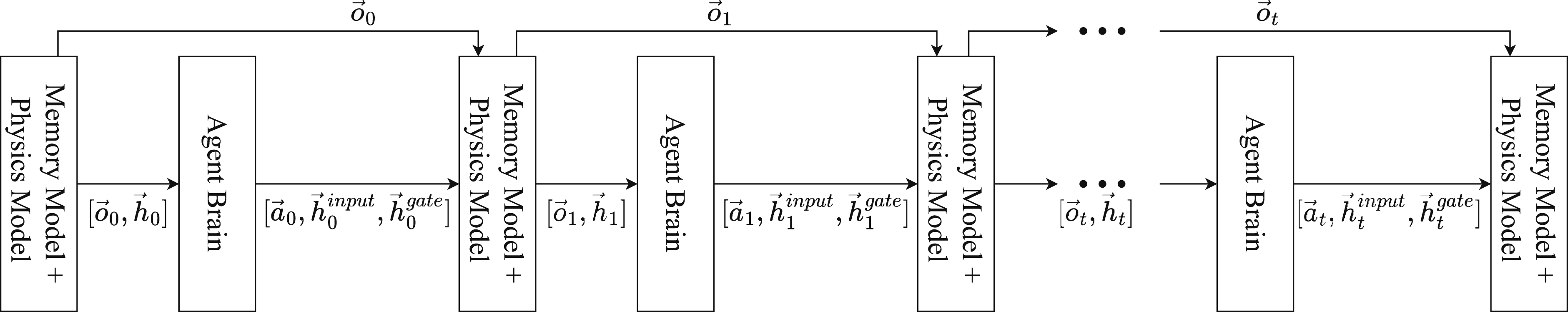

Once the quantity $\partial R / \partial \vec{w}$ is obtained, gradient ascent on R can then be performed to improve the performance of the neural network at maximising R

Δ \vec{w} = α \frac{\partial R}{a \vec{w}}

(7)

where α > 0 is a small learning rate. This single simple process is model-based, that is, requires knowledge of the derivatives of the environment functions (1), (3) and (6). If successful, this learning process will maximise R by (7); hence, this will train the neural network to solve the exploration problem and use the recurrent-memory nodes to execute the exploration algorithm necessary to find and exploit the food pile.

Interestingly, even though knowledge of the food-pile distribution function (1) and physics model (3) is needed to be known during training (by the BPTT algorithm; not by the agent), once the agent has ‘learned how to learn’, access to full knowledge of (1) and (3) is not needed. After training, the agent’s RNN samples exploratory scalar values of the function (3) and then makes decisions based on those samples. It no longer gets or needs access to the derivatives of this function. In this sense, once trained, the ‘inner’ component of the meta-learning system (i.e. the RNN) has learned to perform true model-free RL on the environment (albeit only on this specific food-pile environment). Once trained, and when the RNN is unleashed on the environment, it performs model-free RL to locate and exploit the peak of the food pile.

Experiments

We experimented with two versions of the problem and five selected RL and ADP algorithms. In the first version, we simplified the problem by fixing the distribution of the food pile; this means that exploratory observations are not required to solve the problem. In the second version, we used the full partially observable problem, where the location and height of the food source were randomised, and the agent must make exploratory observations to find the food.

General Experimented Algorithm Setup

The following RL algorithms were used in all experiments: Advantage Actor-Critic (A2C) (Mnih et al., 2016), Soft Actor-Critic (SAC) (Haarnoja et al., 2017), Deep Deterministic Policy Gradient (DDPG) (Lillicrap et al., 2015) and Twin Delayed DDPG (TD3) (Fujimoto et al., 2018). These RL algorithms’ implementations came from the Stable-Baselines package (Raffin et al., 2019) (version 1.1.0). These state-of-the-art algorithms were selected considering their successful history in different benchmark environments (Brockman et al., 2016). Additionally, the implementation of BPTT that we used was our own.

Each algorithm was run for 100,000 iterations, over 20 different trials. The hyper-parameters used by each algorithm were:

• The DDPG, SAC and TD3 algorithms used 100 batches in replay memory with a buffer size of 10⁶. Neural network weights were optimised with an Adam optimiser, with a learning rate of .001. The DDPG algorithm used the soft update coefficient (‘Polyak’ update) of .005, and its default discount factor was .99.

• In the A2C algorithm, we used a discount factor of .99 and a value-function coefficient for the loss calculation of .5. This algorithm used RMSprop optimiser with ϵ = 10⁻⁵. In addition, the A2C algorithm used action noise exploration with an entropy coefficient of .001.

• BPTT used the Adam optimiser with a learning rate of .001, with a discount factor of 1.

For the four main RL algorithms, the above hyper-parameters were the default values provided by the Stable-Baselines package. The learning rates were adjusted to produce optimal results on the initial experiment (i.e. fixed food location experiment). We then transferred these optimal and default hyper-parameters values to use in the second experiment.

The batching method in our BPTT implementation enabled the algorithm to process 100 complete trajectories per iteration (i.e. per update of the weights in the neural network). Since each trajectory (episode) length was L = 30, the BPTT algorithm allowed 3000 environment steps for each weight update. To match this as closely as possible for the selected RL algorithms, we set the hyper-parameters provided in the Stable-Baselines package to be train_frequency = 3000 and gradient_step = −1. This ensures the algorithm updates the weights in the neural network for every 3000 environment interactions taken by the agent. When it does so, these weight updates are accumulated over those 3000 environment steps.

All the selected RL algorithms (DDPG, A2C, SAC and TD3) consist of actor and critic networks. The actor network is structured as described above (see Figure 2).

All of the critic networks used by the RL algorithms were Q-networks. These implement a function $Q : ({\vec{o}}_{t}, {\vec{a}}_{t}) \to R$ . Hence, the critic network has four input nodes (two for ${\vec{o}}_{t}$ , two for ${\vec{a}}_{t}$ ) and one output. There is one hidden layer of 20 tanh nodes (like in Figure 2) and no activation function on the final layer.

The network used in BPTT did not have a critic network, however. Instead, it only required an action network with an identical structure and purpose to the above actor networks.

Simplified Experiment: Fixed Food Location

In this initial simplified experiment, the food pile was fixed at (0,0), with z_food = 1 and σ_food = 8. This initial experiment aims to validate that all the selected ADP/RL algorithms work as intended. The initial agent positions were randomised uniformly at the start of every episode with x ∈ [−5, 5], y ∈ [−5, 5] to prevent memorising a fixed solution.

The environment is fully known in this simplified experiment since the food source is always in the same place, (0,0). Hence, we did not include any recurrent-memory nodes, or the sensor input d (x_t, y_t) in the neural network, as these were not required. The neural-network structure we used in our ADP/RL algorithms consisted of one hidden layer with 20 nodes (like in Figure 2, but without the inputs ${\vec{h}}_{t}$ and d (x_t, y_t), and without the outputs ${\vec{h}}_{t}^{gate}$ and ${\vec{h}}_{t}^{input}$ ). The tanh activation function was used in the hidden layer, and no activation function was used in the output layer.

Full Partial-Observability Experiment: Randomised Food-Pile Location

In this main experiment, the food location was re-randomised at the start of each episode, and the initial agent positions were always started from (0,0). This is the full partial-observability version of the problem, which is necessary for sensing and memory capabilities. Each time an agent starts, the food-pile location was chosen with uniform random distribution such that x_food ∈ [−5, 5], y_food ∈ [−5, 5], z_food ∈ [0.5, 1.5] and σ_food = 8. In addition, we randomised the height of the food source (z_food) within that range to apply further difficulty in this full partial-observability experiment.

The neural network used in this experiment is the same as in the previous experiment, except that now there are now m = 20 recurrent nodes (5a) and also the sensor input d (x_t, y_t) is used in (4).

Compared to the previous experiment, this changed the actor network to have an extra 20 input nodes for ${\vec{h}}_{t}$ and an extra node holding the sensory input (d (x_t, y_t)). The actor-network output was extended by 20 nodes for ${\vec{h}}_{t}^{gate}$ and a further 20 nodes for ${\vec{h}}_{t}^{input}$ , compared to the previous experiment. See Figure 2. The critic network’s input was also extended by 20 nodes for ${\vec{h}}_{t}$ and the extra input node for d (x_t, y_t), and the critic output remained a scalar for holding Q-values.

An interesting implementation detail is that we put the recurrence equation (6) into the environment model and not in our neural network, in accordance with Figures 3 and 4. Under this scheme, the ‘environment’ is treated as a more complicated function, which takes extra inputs ${\vec{h}}_{t}^{gate}$ and ${\vec{h}}_{t}^{input}$ (in addition to the usual state and action inputs), and emits extra output information ${\vec{h}}_{t + 1}$ (in addition to the usual next state and reward, information). The neural network is considered feed-forward (Figure 2).

While this change of view makes no functional difference to the way equations (3b) and (6) behave, from an implementation point of view, it can be useful to put (6) into the environment because it then enables learning algorithms that were not written with recurrent neural networks in mind to be applied to our environment, and to be able to instil the agent with the capabilities of gated recurrent memory.

Results

The following result graphs show the mean value and its 95% confidence intervals calculated over 20 trials by the ‘Seaborn’ software library. Figure 5 shows that BPTT solved the simplified version of the problem stably and robustly. However, the selected state-of-the-art RL algorithms also did approximately solve the problem but did not perform as rapidly and did not achieve stable learning or the same final total reward as was achieved by BPTT.

Figure 5.

Algorithms’ performance on fixed food location validation environment over 100,000 iterations and averaged over 20 trials.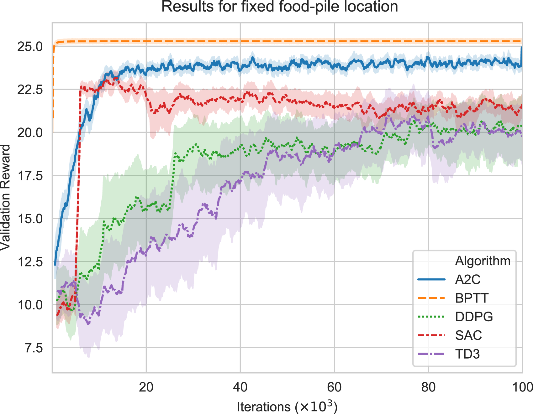

From the final iteration results shown in Figure 5, we selected a sample of 10 trajectories created by our agent trained by BPTT. Next, we visualised their movement behaviour in Figure 6. The circles in Figure 6 show the starting point of the agents, and the crosses represent the goal points in the environment space. The arrows show the direction of the moving agents; this shows them precisely moving towards the fixed food-source location in straight lines.

Figure 6.

Top-down view of BPTT results for the simplified experiment (with no sensor or recurrent memory). The x and y axes describe the location. Each different coloured pathway represents a trajectory starting from a different coloured spot. All trajectories end up at the food-pile location (0,0).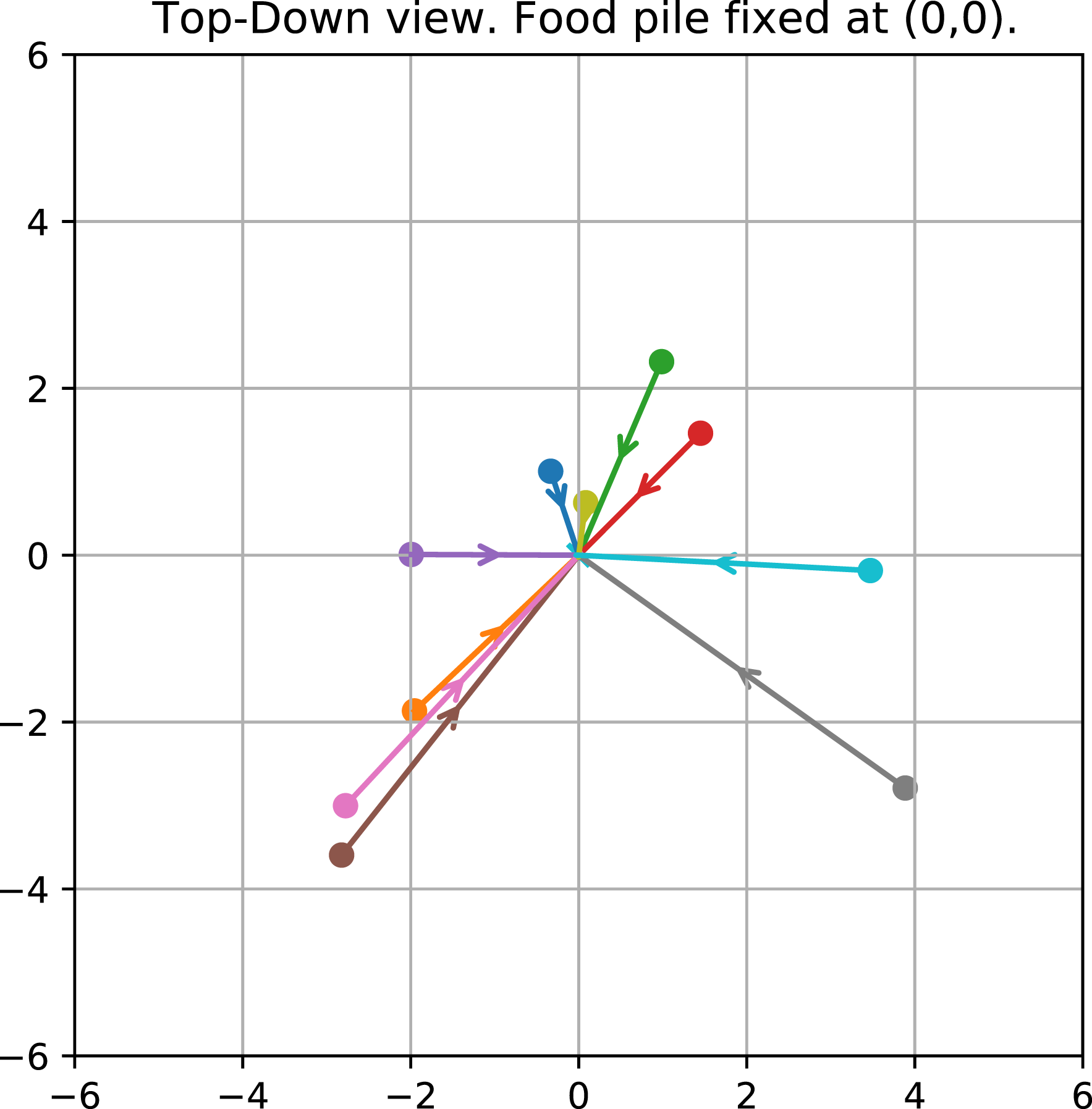

According to Figure 6, it can be seen that the BPTT agent navigates towards the goal optimally. This shows that the average reward (25.5) achieved by the BPTT method in Figure 5 is a significant target to aim for in the following experiment.

The results are shown in Figure 7 for this full partial-observability experiment. The selected RL algorithms struggled to perform well and devise a navigational strategy to find the peak of the food pile. Nevertheless, they achieved between 6 and 12.5 maximum average rewards, showing that the agents did not explore properly and got stuck in the same local region. However, the BPTT algorithm reached around 22.5 maximum average rewards, indicating that the BPTT agents solved the problem.

Figure 7.

Algorithms’ performance on randomised food location validation environment over 100,000 iterations and averaged over 20 trials. Each algorithm used sensory data input and 20 recurrent nodes.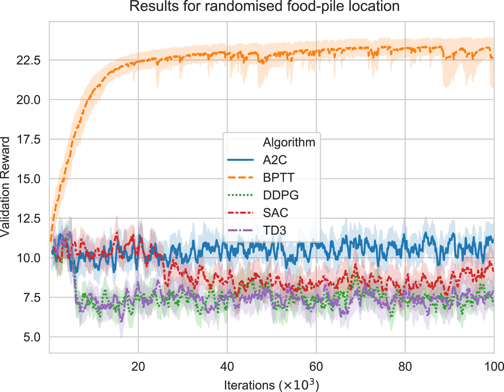

The score attained by BPTT is close to the maximum score of 25.5, which was attained in the simplified experiment, indicating that the BPTT agent is close-to-optimal in the partially observable environment. Furthermore, there is a symmetry between the two situations (even though the arrows are reversed between Figures 6 and 8(a)), which indicates that the maximum reward attainable should be roughly the same between the two situations. There is a slight reduction in performance in comparison, though (i.e. 22.5 $<$ 25.5), as each agent in the full partial-observability problem needs to spend some initial time exploring before it can head quickly to the top of the food pile.

Figure 8.

Behaviour of fully trained BPTT agents at solving the randomised food-pile problem on a test set. The x and y axes describe the location. Each coloured pathway represents a trajectory from the common start point at (0,0). These show the agents exploring and calculating the direction of increasing food density and then travelling to the food-pile peaks. Each different coloured trajectory ends up at or near the centre of its own specific food-pile location (indicated by the coloured X symbols).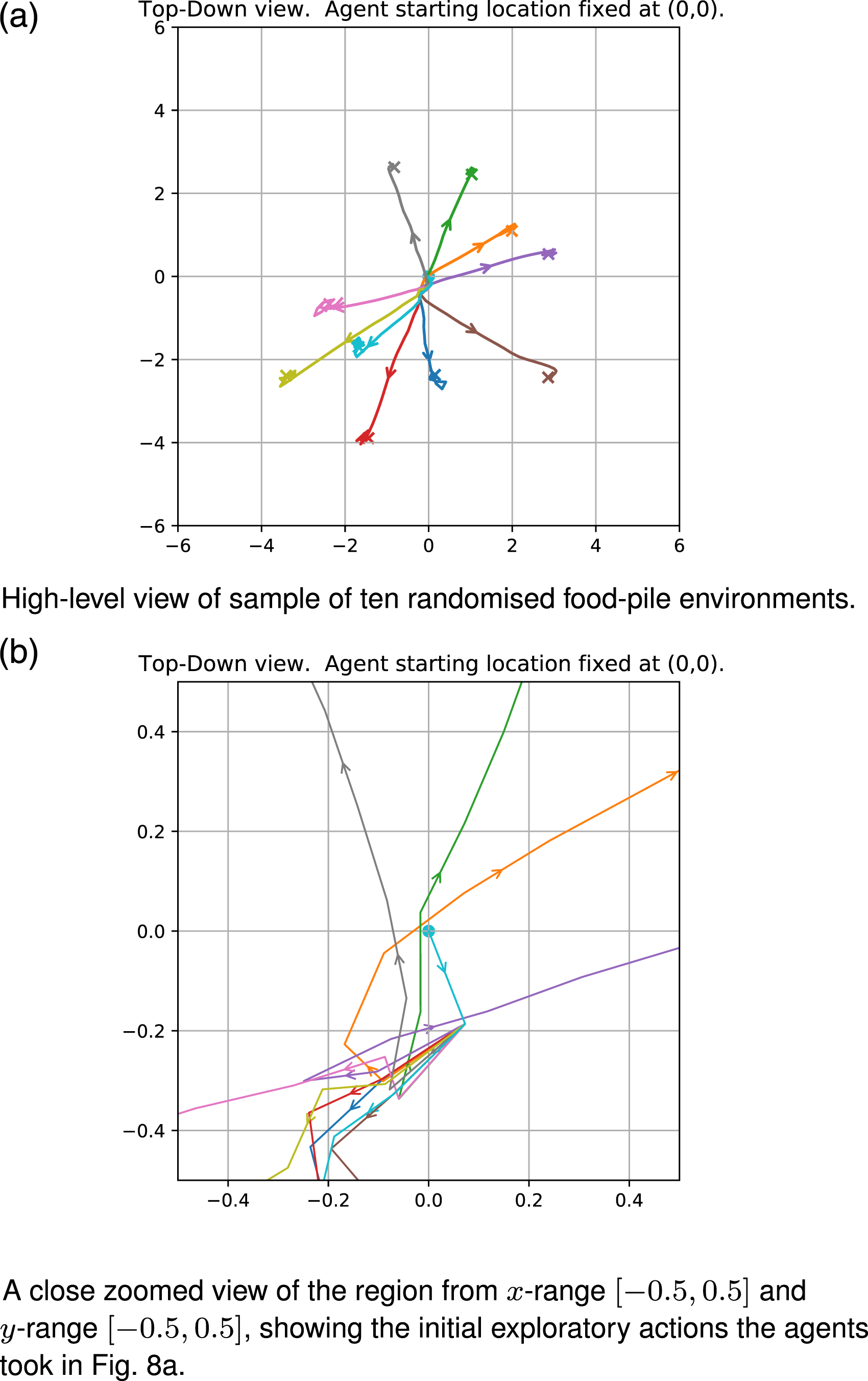

Figure 8(a) shows a sample of 10 trajectories from the fully trained BPTT agent’s behavioural movement. Figure 8(b) shows a close-up zoom of the central region, highlighting the agents performing an exploration strategy to reach the goal.

Figure 8(b) shows that the RNN exploration algorithm learned to navigate and devise a movement strategy using input sensory data and memory. It illustrates that the 10 sample trajectories created by the BPTT agents started from (0,0), with a break-off point around (0.1, −0.19). From that separation point, it showed that the RNN’s memories of previous observations affect our agents’ decisions after sampling multiple sensor results.

We performed an ablation study using three different versions of the neural-network architecture to clarify that recurrent memories and a sensor were required for the BPTT algorithm to solve the randomised food-location environment. These different versions involved removing the sensor and/or the recurrent memory. The results are shown in Figure 9 and conclude that the recurrent-memory nodes and sensor input are necessary for solving the navigational task.

Figure 9.

The effect of solving the randomised food-pile location problem with and without sensors and memory is that each algorithm setup is experimented with over 10,000 iterations and averaged over 20 different trials.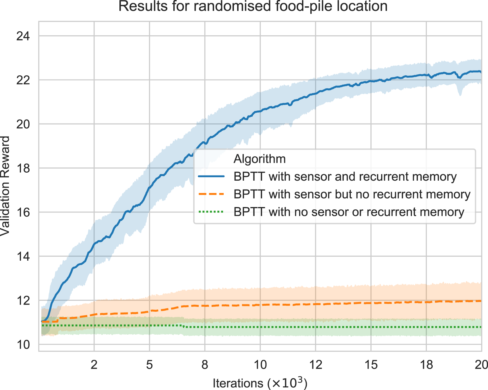

Discussion

In our experiments, BPTT showed competency in performance and stability in both the simplified and in the partially observable environments. The BPTT algorithm discovered an exploration method that looks like the agent is wobbling as it moves towards the goal. This wobble at the start can be assumed to be the agent taking exploratory actions, that is, it has successfully learned how to learn. The other RL algorithms could only solve the fixed food location problem, but failed to scale up to the full partially observable randomised food-pile problem. In the simplified experiment, the selected RL algorithms had poorer performance than the BPTT algorithm seen in Figure 5. This is partly due to the RL algorithms always needing to embed stochastic exploration into their actions. Another reason is that they cannot exploit true gradient information through the environment model when learning, which BPTT benefits from.

It appears in Figures 5 and 7 that at the start of training, the agents receive an average validation reward of approximately 10. This is explained because for an average randomisation of the initial agent and food positions if the agents were to stand still for 30 time-steps. Then, they would receive an average total reward of 10.7 (a value we found in a separate informal experiment).

Figures 5 and 7 show that the reward progression does not consistently show monotonic improvement, especially with the RL algorithms. This is likely because the RL algorithms are not proven to be true gradient ascent on any objective function, in contrast to BPTT (Barnard, 1993; Fairbank et al., 2013).

Figure 7 shows that the selected RL algorithms failed to devise any movement strategy that improved on the initial average reward of 10.7. Their agents got stuck in the same region and did not successfully apply exploration strategies.

This might be because the recurrent memory and the sensory-input features uniquely benefited the BPTT algorithm. However, the selected RL algorithms are sensitive to hyper-parameters chosen to solve RL-based problems. Unfortunately, we could not find any combination of hyper-parameters to see any improvements. However, our successful initial fixed food-pile experiment (Figure 5) using the RL algorithms with the same hyper-parameters indicates that the hyper-parameters we used were at least reasonable.

One interesting trajectory in Figure 8(b) is the purple line which shows a complete turnaround at approximately (−0.25, −0.3) as the agent ‘realises’ it set off in the wrong direction. This systematic exploration method and multiple sampling of the food density from different locations allow the RNN to deduce the direction in which the food density increases the most. The agent (RNN) learns during an episode (the ‘inner’ learning algorithm).

The pathways over the food hill taken by our BPTT agents indicate that the agents’ RNNs have discovered an exploration algorithm that samples and records food heights in the environment and acts accordingly. Furthermore, the BPTT algorithm (the ‘outer algorithm’) has chosen weights that enabled the RNN to behave like this. This adaptive behaviour is consistent with the minimal simulated ‘organism’ approach favoured in this work. To solve the full partial-observability experiment, the ablation study in Figure 9 shows that our implemented BPTT algorithm requires recurrent memory combined with sensory-based information. The other two variants of the implemented BPTT (BPTT with no sensor or recurrent memory, and BPTT with sensor and no recurrent memory) failed to solve the problem.

In the partially observable environment, we forced all algorithms to obey our recurrent-memory equation (6) by embedding those equations within the environment model. Although this combined system (of physics plus memory) is a valid ‘environment’, it turned out to be a particularly challenging one that the RL algorithms could not cope with.

In contrast, the BPTT algorithm exploits knowledge of the true derivatives which pass through the physics environment, through the memory model, and the neural network, that is, back-propagating gradients right through the unrolled network shown in Figure 4; and these derivatives seem to have been crucial in correctly solving this exploration problem. It seems a reasonable explanation that gradient-based algorithms such as BPTT can potentially extract more information quickly from an environment than scalar-based model-free RL methods (Fairbank and Alonso 2012).

Conclusion

Using a sensor and recurrent-memory capabilities, we have presented a simple simulated ‘organism’ with an exploratory task to solve a food-gathering problem in a partial-observable and differentiable environment. Our full partial-observability experiment showed that the agent learned to learn with fixed RNN weights. This matches the definition of meta-learning given by Prokhorov et al. (2002) and Younger et al. (2001), and the definition of ‘accommodative neural networks’ by Lo and Bassu (2001).

We found this opportunity to emphasise the potential benefits of BPTT on neural control and demonstrate its performance on navigational tasks with limited observable signals in a continuous-state environment. BPTT can negotiate the exploration-exploitation trade-off, and with the evaluation of the entire trajectory, the average reward improves the agent’s policy using a reward-based policy update.

The ablation study in Figure 9 confirms that both the use of memories and sensor observations are necessary to solve this task. Furthermore, the trajectories shown in Figure 8(a) are fairly direct, indicating that any initial triangulation calculation made by the RNN must have been fairly accurate. This suggests a purposefulness of the goal seeking, which is in contrast to a simpler stochastic hill-climbing algorithm, which might be expected to show random ‘jittering’ throughout the length of the trajectory.

These conclusions indicate that our agent must possess all five numbered sentient-creature attributes listed in the introduction.

Out of the algorithms considered, only the BPTT algorithm could successfully produce a working RNN. The fact that the solution is self-learned is beneficial because, in principle, without any further modification, the self-learning method could create any other RNN algorithm of similar complexity for different tasks.

BPTT is an ADP algorithm that uses the physics model and its derivatives to enable rapid learning. The other selected state-of-the-art algorithms used in the experiments are ‘true’ RL, where the physics model is separated from the learning model, and the agent learns in a separated interactive environment by trial and error. Despite this limitation of BPTT that requires access to the physics-model derivatives during training, we argue that once created by the BPTT algorithm, the final RNN created does not require any access to these derivatives and that the RNN executes a model-free algorithm to explore and exploit the environment.

In future work, it would be possible to investigate more elaborate food distributions and partial observability than that shown in Figure 1, possibly while enhancing the sensory capabilities of the agent. It would also be possible to investigate alternative memory mechanisms to (6), such as incorporating a full GRU (Cho et al., 2014), LSTM (Hochreiter and Schmidhuber 1997) or the content-adaptive recurrent units (CARU) (Chan et al., 2020).

Finally, since the selected RL algorithms failed to show improvements in our experiments, exploring state-of-the-art RL algorithms is suggested to understand their performance in tackling full partial-observable environments and enable them to benefit from gradient-based learning through their recurrent-memory nodes.

Footnotes

Declaration of conflicting interests

The author(s) declared no potential conflicts of interest with respect to the research, authorship, and/or publication of this article.

Funding

The author(s) disclosed receipt of the following financial support for the research, authorship, and/or publication of this article: This research was partially supported by the Business and Local Government Data Research Centre BLG DRC (ES/S007156/1) and by the ESRC Research Centre on Micro-Social Change (MiSoC) - ES/S012486/1, both funded by the Economic and Social Research Council (ESRC).

ORCID iD

Mahrad Pisheh Var

Note

About the Authors

Mahrad Pisheh Var is a highly motivated PhD student who is currently conducting research under the supervision of Michael Fairbank in the field of neuro control. He obtained his undergraduate degrees in Computer Science and Computer Games with a 1st and a distinction respectively from the University of Essex. He is passionate about discovering novel gradient-based techniques for training neural networks and believes that there is a great potential for improving AI to converge quickly. Mahrad moved to the United Kingdom at the age of 17 and has since accomplished numerous academic achievements. He has gained invaluable experience in developing his own game engine from scratch and working with cutting-edge technologies such as AIs and BCIs brain computer interfaces. With his strong academic background and practical experience in the field, Mahrad is well-positioned to make significant contributions to the field of neuro control and AI.

Michael Fairbank is a senior lecturer and researcher in learning algorithms for adaptive dynamic programming and neural networks, at the University of Essex, UK. He received his Ph.D. from City University of London in 2014, B.Sc. degree in Mathematical Physics from Nottingham University in 1994, and M.Sc. in Knowledge Based Systems from Edinburgh University in 1995.

Spyridon Samothrakis is a Senior Lecturer and Deputy Director of the Institute for Analytics and Data Science at the University of Essex. He obtained his PhD in Computer Science in 2014, focusing on optimal game playing in multi-player games. Dr Samothrakis has worked extensively with businesses and his current research interests are meta-learning and reinforcement learning.

References

Barnard

(1993). Temporal-difference methods and markov models. IEEE Transactions on Systems, Man, and Cybernetics, 23(2), 357–365. https://doi.org/10.1109/21.229449

Beer

R. D.

(2003). The dynamics of active categorical perception in an evolved model agent. Adaptive Behavior, 11(4), 209–243. https://doi.org/10.1177/1059712303114001

Braitenberg

(1986). Vehicles: Experiments in synthetic psychology. MIT press.

Braun

D. A.

Aertsen

Wolpert

D. M.

Mehring

(2009). Learning optimal adaptation strategies in unpredictable motor tasks. The Journal of Neuroscience: The Official Journal of the Society for Neuroscience, 29(20), 6472–6478. https://doi.org/10.1523/JNEUROSCI.3075-08.2009

Brockman

Cheung

Pettersson

Schneider

Schulman

Tang

Zaremba

(2016). OpenAi gym. arXiv preprint arXiv:1606.01540.

Chan

K. H.

S. K.

(2020). Caru: A content-adaptive recurrent unit for the transition of hidden state in nlp. In International conference on neural information processing (pp. 693–703). Springer.

Cho

Van Merriënboer

Bahdanau

Bengio

(2014). On the properties of neural machine translation: Encoder-decoder approaches. 103–111. Association for Computational Linguistics. arXiv preprint arXiv:1409.1259.

Chung

Gulcehre

Cho

Bengio

(2014). Empirical evaluation of gated recurrent neural networks on sequence modeling. arXiv preprint arXiv:1412.3555.

Chung

Siegelmann

(2021). Turing completeness of bounded-precision recurrent neural networks. Advances in Neural Information Processing Systems, 34, 28431–28441.

10.

Conway

(1970). The game of life. Scientific American, 223(4), 4.

11.

Cotter

N. E.

Conwell

P. R.

(1990). Fixed-weight networks can learn. In 1990 IJCNN international joint conference on neural networks (pp. 553–559). IEEE.

12.

Fairbank

Alonso

(2012). A comparison of learning speed and ability to cope without exploration between DHP and TD (0). In The 2012 international joint conference on neural networks (IJCNN) (pp. 1–8). IEEE.

13.

Fairbank

Alonso

Prokhorov

(2012). Simple and fast calculation of the second-order gradients for globalized dual heuristic dynamic programming in neural networks. IEEE Transactions on Neural Networks and Learning Systems, 23(10), 1671–1676. https://doi.org/10.1109/TNNLS.2012.2205268

14.

Fairbank

Alonso

Prokhorov

(2013). An equivalence between adaptive dynamic programming with a critic and backpropagation through time. IEEE Transactions on Neural Networks and Learning Systems, 24(12), 2088–2100. https://doi.org/10.1109/TNNLS.2013.2271778

15.

Fairbank

Alonso

Wunsch

(2014). An adaptive recurrent neural-network controller using a stabilization matrix and predictive inputs to solve a tracking problem under disturbances. Neural Networks, 49, 74–86. https://doi.org/10.1016/j.neunet.2013.09.010

16.

Fairbank

Prokhorov

Alonso

(2014). Clipping in neurocontrol by adaptive dynamic programming. IEEE Transactions on Neural Networks and Learning Systems, 25(10), 1909–1920. https://doi.org/10.1109/TNNLS.2014.2297991

17.

Finn

Abbeel

Levine

(2017). Model-agnostic meta-learning for fast adaptation of deep networks. In International conference on machine learning (pp. 1126–1135). PMLR.

18.

Fairbank

Wunsch

D. C.

Alonso

(2015). Training recurrent neural networks with the levenberg–marquardt algorithm for optimal control of a grid-connected converter. IEEE Transactions on Neural Networks and Learning Systems, 26(9), 1900–1912. https://doi.org/10.1109/TNNLS.2014.2361267

19.

Fujimoto

Hoof

Meger

(2018). Addressing function approximation error in actor-critic methods. In International conference on machine learning (pp. 1587–1596). PMLR.

20.

Graves

Wayne

Danihelka

(2014). Neural turing machines. arXiv preprint arXiv:1410.5401.

21.

Haarnoja

Tang

Abbeel

Levine

(2017). Reinforcement learning with deep energy-based policies. In International conference on machine learning (pp. 1352–1361). PMLR.

22.

Hausknecht

Stone

(2015). Deep recurrent Q-learning for partially observable MDPs. In 2015 aaai fall symposium series. AAAI Press.

23.

Hochreiter

Schmidhuber

(1997). Long short-term memory. Neural Computation, 9(8), 1735–1780. https://doi.org/10.1162/neco.1997.9.8.1735

24.

Hochreiter

Younger

A. S.

Conwell

P. R.

(2001). Learning to learn using gradient descent. In International conference on artificial neural networks (pp. 87–94). Springer.

25.

(2014). Behaviors and strategies of bacterial navigation in chemical and nonchemical gradients. PLoS Computational Biology, 10(6), e1003672. https://doi.org/10.1371/journal.pcbi.1003672

26.

Kaelbling

L. P.

Littman

M. L.

Cassandra

A. R.

(1998). Planning and acting in partially observable stochastic domains. Artificial Intelligence, 101(1-2), 99–134. https://doi.org/10.1016/s0004-3702(98)00023-x

27.

Zhou

Chowdhury

K. R.

Meleis

(2019). QTCP: Adaptive congestion control with reinforcement learning. IEEE Transactions on Network Science and Engineering, 6(3), 445–458. https://doi.org/10.1109/tnse.2018.2835758

28.

Lillicrap

T. P.

Hunt

J. J.

Pritzel

Heess

Erez

Tassa

Silver

Wierstra

(2015). Continuous control with deep reinforcement learning. arXiv preprint arXiv:1509.02971.

29.

Lillicrap

T. P.

Santoro

(2019). Backpropagation through time and the brain. Current Opinion in Neurobiology, 55, 82–89. https://doi.org/10.1016/j.conb.2019.01.011

30.

J. T.

Bassu

(2001) Adaptive vs. accommodative neural networks for adaptive system identification. In IJCNN’01. International Joint Conference on Neural Networks. Proceedings (Cat. No. 01CH37222), volume 2, 1279–1284, NJ, USA, IEEE.

31.

Mnih

Badia

A. P.

Mirza

Graves

Lillicrap

Harley

Silver

Kavukcuoglu

(2016). Asynchronous methods for deep reinforcement learning. In International conference on machine learning (pp. 1928–1937). PMLR.

32.

Mnih

Kavukcuoglu

Silver

Graves

Antonoglou

Wierstra

Riedmiller

(2013). Playing atari with deep reinforcement learning. DeepMind Technologies. arXiv preprint arXiv:1312.5602.

33.

Murray

J. J.

Cox

C. J.

Lendaris

G. G.

Saeks

(2002). Adaptive dynamic programming. IEEE Transactions on Systems, Man, and Cybernetics, Part C (Applications and Reviews), 32(2), 140–153. https://doi.org/10.1109/tsmcc.2002.801727

34.

Nichol

Schulman

(2018) Reptile: A scalable metalearning algorithm. Artificial Intelligence, 2(3), 4. arXiv preprint arXiv:1803.02999.

35.

Ortega

P. A.

Wang

J. X.

Rowland

Genewein

Kurth-Nelson

Pascanu

Heess

Veness

Pritzel

Sprechmann

, et al. (2019). Meta-learning of sequential strategies. arXiv preprint arXiv:1905.03030.

36.

Prince

L. Y.

Eyono

R. H.

Boven

Ghosh

Pemberton

Scherr

Clopath

Costa

R. P.

Maass

Richards

B. A.

, et al. (2021). Current state and future directions for learning in biological recurrent neural networks: A perspective piece. arXiv preprint arXiv:2105.05382.

37.

Prokhorov

D. V.

Feldkarnp

Tyukin

I. Y.

(2002) Adaptive behavior with fixed weights in RNN: An overview. In Proceedings of the 2002 international joint conference on neural networks. IJCNN’02 (Cat. No. 02CH37290), volume 3, pp. 2018–2022, NJ, USA, IEEE.

38.

Prokhorov

D. V.

Wunsch

D. C.

(1997). Adaptive critic designs. IEEE Transactions on Neural Networks, 8(5), 997–1007. https://doi.org/10.1109/72.623201

39.

Raffin

Hill

Ernestus

Gleave

Kanervisto

Dormann

(2019). Stable baselines3. https://github.com/DLR-RM/stable-baselines3

40.

Santoro

Bartunov

Botvinick

Wierstra

Lillicrap

(2016). Meta-learning with memory-augmented neural networks. In International conference on machine learning (pp. 1842–1850). PMLR.

41.

Schaul

Schmidhuber

(2010). Metalearning. Scholarpedia, 5(6), 4650. https://doi.org/10.4249/scholarpedia.4650

42.

Silver

Hubert

Schrittwieser

Antonoglou

Lai

Guez

Lanctot

Sifre

Kumaran

Graepel

Lillicrap

Simonyan

Hassabis

(2018). A general reinforcement learning algorithm that masters chess, shogi, and go through self-play. Science, 362(6419), 1140–1144. https://doi.org/10.1126/science.aar6404

43.

Stadie

B. C.

Yang

Houthooft

Chen

Duan

Abbeel

Sutskever

(2018). Some considerations on learning to explore via meta-reinforcement learning. arXiv preprint arXiv:1803.01118.

44.

Sutton

R. S.

Barto

A. G.

(2018). Reinforcement learning: An introduction. MIT press.

45.

Teichmann

(2015). Models of aposematism and the role of aversive learning. [PhD Thesis City University London].

46.

Thrun

Pratt

(1998). Learning to learn: Introduction and overview. In Learning to learn (pp. 3–17). Springer.

47.

Wang

F. Y.

Zhang

Liu

(2009). Adaptive dynamic programming: An introduction. IEEE Computational Intelligence Magazine, 4(2), 39–47. https://doi.org/10.1109/mci.2009.932261

48.

Werbos

P. J.

(1990). Backpropagation through time: What it does and how to do it. Proceedings of the IEEE, 78(10), 1550–1560. https://doi.org/10.1109/5.58337

49.

Wierstra

Foerster

Peters

Schmidhuber

(2007). Solving deep memory POMDPs with recurrent policy gradients. In International conference on artificial neural networks (pp. 697–706). Springer.

50.

Wierstra

Förster

Peters

Schmidhuber

(2010). Recurrent policy gradients. Logic Journal of IGPL, 18(5), 620–634. https://doi.org/10.1093/jigpal/jzp049

51.

Younger

A. S.

Conwell

P. R.

Cotter

N. E.

(1999). Fixed-weight on-line learning. IEEE Transactions on Neural Networks, 10(2), 272–283. https://doi.org/10.1109/72.750553

52.

Younger

A. S.

Hochreiter

Conwell

P. R.

(2001). Meta-learning with backpropagation. IJCNN’01. International Joint Conference on Neural Networks. Proceedings (Cat. No. 01CH37222. (volume 3). 1098–7576, NJ, USA, IEEE.

53.

Zhou

G. B.

Zhang

C. L.

Zhou

Z. H.

(2016). Minimal gated unit for recurrent neural networks. International Journal of Automation and Computing, 13(3), 226–234. https://doi.org/10.1007/s11633-016-1006-2

A Minimal “Functionally Sentient” Organism Trained With Backpropagation Through Time

Abstract

Keywords

Introduction

Related Work

Tackling Partially Observable Environments

Meta-Learning

Adaptive Dynamic Programming

Environment and Agent Definitions

Environment Rewards

Agent’s Physics

Agent Brain

Backpropagation Through Time Algorithm

Experiments

General Experimented Algorithm Setup

Simplified Experiment: Fixed Food Location

Full Partial-Observability Experiment: Randomised Food-Pile Location

Results

Discussion

Conclusion

Footnotes

Declaration of conflicting interests

Funding

ORCID iD

Note

About the Authors

References