Optimality of Base-Stock Policy Under Unknown General Demand Distributions: New Methods,New Results,and Computations

Abstract

This article advances the literature on the optimality of the base-stock policy for a general demand distribution and a general prior belief, which we update as we observe realized demands, assumed to be continuous, independent and identically distributed, random variables. The value function depends on the belief, so the functional Bellman equation is infinite-dimensional. Significantly, in contrast with traditional approaches, we derive a functional equation for the derivative of the value function with respect to the inventory level, which provides a direct approach to computing the optimal base-stock policy. In two well-known cases, we characterize how the base-stock level depends on the belief, and we implement the approach to compute the optimal base-stock level. In the first case of conjugate probabilities, the infinite-dimensional state reduces to a finite-dimensional sufficient statistic. That allows us to solve two numerical examples of exponential and Weibull demands. Moreover, for the exponential demand example, we compare the optimal cost with the costs achieved by two myopic policies with three guesses of the initial belief. We find that the optimal policy improves upon the first myopic policy by 12.6%, 13.0%, and 9.2%, and upon the second myopic policy by 28.7%, 26.9%, and 27.7%. The second case considers the demand to come from one of two possible distributions, but we do not know which. Here, we derive a functional equation in one hyperparameter expressing the ratio of the weights assigned to the two distributions. We then develop an approximation scheme to solve it, show that it converges, and implement it numerically to obtain the optimal base-stock levels over time.

1. Introduction

We consider a discrete-time infinite-horizon inventory problem with demand depending on an unknown parameter and allowing for backlogging of unmet demands, which makes the realized demands fully observed (Section 3). A Bayesian framework is often used to study such problems when intuition and previous experience supply a prior parameter distribution. Bayes’ rule provides a way to incorporate new information (observed demands in our case) into the decision model as it becomes available. As far back as 1959, Herbert E. Scarf studied this problem in the case of exponential demand and showed that a base-stock policy is optimal with the base-stock level depending on a single sufficient statistic—the mean of past demand observations. Scarf (1959) first uses dynamic programming to study the finite-horizon version of the problem and then treats the infinite-horizon version using an asymptotic analysis. He mentions that the base-stock functions are difficult to obtain analytically, so he focuses on their properties and asymptotic expansion under some regularity conditions.

Since inventory managers do not fully know the demand distribution in many practical situations and the problem is exciting and theoretically challenging, many well-known authors have built upon the work of Scarf (1959, 1960) in several notable demand cases. Early ones include Azoury (1985), Iglehart (1964), Karlin (1960), and Lovejoy (1990). However, they studied only finite-horizon problems, not the stationary infinite-horizon problems we study. We review the more recent relevant literature in Section 2 and tangentially related literature in EC.1 (Section EC.1 in the E-Companion). We make several contributions to the literature.

1.1. We advance the extant literature by assuming a general demand distribution depending on an unknown parameter and a general initial belief about the unknown parameter. Then, the state equation evolves in the infinite-dimensional state space of the current inventory and belief density, which gets updated as the demand history unfolds. We show rigorously that the optimal ordering policy is a base-stock policy with the base-stock level dependent on the current infinite-dimensional belief density of the unknown parameter. In contrast, this result has been rigorously established only for finite-horizon problems in particular demand cases in the literature.

1.2. We consider an infinite-horizon setting, which is quite helpful in practice as it dispenses the time argument when accounting for future periods and thus brings the advantage of a single period setting. But then, we must solve a functional Bellman equation instead of considering a sequence of functions indexed by time. The study of the functional equation is direct, without first solving a finite horizon problem and then going to the limit.

Consequently, our subsequent analysis represents significant methodological contributions that are more generally applicable. The Bellman equation for our problem is a functional equation in an infinite-dimensional space. To facilitate its study, we enlarge the domain of belief functions to positive integrable functions, called unnormalized probabilities, which are not necessarily probability densities. This procedure results in an equivalent unnormalized Bellman equation, and its state is a finite-dimensional inventory and an unnormalized infinitely dimensional belief regarding the parameter. As a result, the unnormalized Bellman equation becomes more straightforward to analyze.

Zakai (1969) introduced the concept of unnormalized probability in the nonlinear filtering theory. It was first applied to partially observed inventory problems by Bensoussan et al. (2007) to establish the existence and uniqueness of the solution of the Bellman equation. While this methodology is efficient for the value function in terms of establishing the existence and uniqueness of the solution of the Bellman equation and was later used by Bensoussan et al. (2008a, 2008b, 2009) and Bensoussan and Guo (2015) for that purpose, it does not easily give the optimal feedback policies one looks for in stochastic control problems.

1.3. Even though our analysis of the Bellman equation has similarities with the above works in which the state is the infinite-dimensional belief, there is an essential difference in the sense that our state is mixed, consisting of the finite-dimensional inventory and the exogenous infinite-dimensional belief. Because we allow backlogging, we can observe realized demands, so the belief evolution does not depend on inventory observations. However, these enable us to obtain the optimal feedback policy, which is a base-stock policy with the base-stock level depending on the current belief.

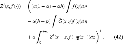
1.4. Since the Bellman equation involves an inf operation to obtain the optimal policy, we must differentiate the unnormalized value function with respect to inventory. Then, why not derive a functional equation for the requisite derivative rather than obtain the value function and take its derivative? If we can, the advantage would be that we can work on a space of bounded functionals on a functional space and rely on a contraction mapping theorem to obtain the derivative directly as the fixed point of an equation (namely, (42) in Subsection 6.3) by an iterative procedure. Once we have this derivative, we can obtain the base-stock level as a function of the belief specified in (40) in Subsection 6.3. Also, while solving for the value function is no longer necessary to obtain the optimal policy, we can compute it if needed. This innovative and constructive approach to obtaining the base-stock level has beneficial monotonicity properties specified in (47) and (49) in Subsection 6.3. These properties facilitate the development of an iterative procedure, which we write for the general case in EC.6.4 (Subsection EC.6.4 in the E-Companion). The procedure yields a monotonic decreasing sequence of nonnegative threshold values converging to the belief-dependent base-stock level. As we get a new demand observation each period, we update the belief and use the procedure offline to obtain the base-stock level for the next period.

Scarf (1959) mentioned the difficulty of obtaining base-stock functions analytically for the problems we consider. Lovejoy (1990) stated that these problems are more complicated to solve than the ones with known demand distributions and will not yield simple operational policies. By simple operational policies, he meant policies based on the critical fractile. Since the optimal policies for the problems are base-stock policies, we interpret that to mean that the optimal base-stock levels are challenging to obtain. No wonder the literature provides no computational procedures for computing optimal base-stock levels, even if we limit ourselves to parameterized distributions! The main difficulty is that we cannot solve the Bellman equations to obtain the value functions analytically, making it extremely difficult to take their derivatives as the next step for obtaining the optimal base-stock levels.

Thus, coming up with a contraction mapping for the derivative of the value function, which enables us to obtain the base-stock level for the current belief directly, is very significant. Moreover, the fact that we can obtain a self-contained equation for the derivative of the value function by differentiating the Bellman equation is peculiar to Bellman equations and not well known. We take advantage of it since, in general, there is no reason why differentiating a functional equation would yield a self-contained equation for its derivative. Our approach finesses that for the first time, by computing the derivative of the value function directly as a fixed point of a contraction mapping. We apply our approach to a few particular cases as described below.

1.5. We treat two particular cases when the belief function depends on some hyperparameters. Then, the underlying infinite-dimensional problems become finite-dimensional ones, the dimension being the number of hyperparameters. A popular choice of the belief density is to choose the conjugate-prior for the demand density. We can then express the belief in terms of its hyperparameters that can be updated based on the observed demands, and thus, the base-stock level becomes a function of this sufficient statistic. So, our first particular case is that of well-known Weibull demand whose scale parameter is unknown and whose conjugate-prior is the family of Gamma densities characterized by two hyperparameters. We represent the base-stock level in terms of these two hyperparameters and obtain them numerically. We apply our approach to two particular examples of Weibull demand. For each example, we create demands for 1,000 periods according to an assumed true distribution, start with an initial belief about the hyperparameters, update them using simulated demands following the true demand distribution, obtain the sequence of the optimal base-stock levels over the periods in terms of the updated hyperparameters, and see its march toward the base-stock level, which turns out, as it should, to be the optimal level in the corresponding infinite-horizon problem with the true demand distribution known with certainty. In the remainder of the article, we shall refer to this level for brevity as the asymptotic base-stock level. To save space, we tabulate the optimal base-stock levels in the examples only for the first five periods.

Our second particular case is new to the related literature, and we can treat it since our model allows for general demands and general beliefs. This case considers the demand to come from one of two possible distributions, but we do not know which. Here, we can work with a single hyperparameter expressing the ratio of the weights assigned to the two distributions. We use our theory to write the functional equation satisfied by the derivative of the value function, develop an approximation scheme to solve for the derivative, and obtain the optimal base-stock level in each period. We also illustrate this scheme by numerically solving an example involving high or low exponential demand distributions and tabulating the results.

1.6. Lastly, we compare our method to two critical fractile approaches in the exponential demand case. Lovejoy (1990), recognizing the difficulty of solving the problems under consideration, analytically explores the critical fractile policies. He referred to them as myopic policies according to Sobel (1981), who defined a policy as myopic if it can be deduced from an optimum of a static problem. We implement the critical fractile policies on a rolling horizon basis, as by Avci et al. (2020) and Treharne and Sox (2002). We obtain the current updated demand distribution in each period and use the critical fractile formula to determine the base-stock level. In our first myopic policy, the updated distribution in our exponential demand case is the gamma distribution, given the hyperparameter values. For our second myopic policy, we can ask why not use a procedure that seeks updated distributions within the exponential class. We can accomplish this by beginning with an initial belief about the mean demand and updating it each time we observe a new demand. Fortunately, we already have the updated mean demand given by a ratio of the two hyperparameter values. Since the mean demand is a sufficient statistic for the exponential distribution, we can use it to obtain the critical fractile base-stock level. As expected, our comparison finds that the optimal policy achieves the best cost, albeit using slightly more computational time than the two myopic policies (see Subsection 7.3).

The plan of this article is as follows. Section 2 reviews the related literature. In Section 3, we formulate an inventory problem with the demand depending on a parameter, introduce a general belief density, and use Bayesian learning to update it based on the demands observed over time. In Section 4, we use dynamic programming to obtain the functional Bellman equation and bounds on its solution to ensure a unique solution. In Section 5, we unnormalize the Bellman equation, prove that the value function is the only solution to the Bellman equation, and show that an optimal state-dependent (feedback) policy exists. Section 6 derives the functional equation for the derivative of the value function, shows that the optimal policy is a base-stock policy where the base-stock level depends only on the current belief function, and develops an iterative procedure to obtain the base-stock level. In Section 7, we treat the particular case of conjugate probabilities with the belief modeled by the conjugate-prior of the demand distribution and characterize the base-stock-level’s dependence on the belief distribution’s hyperparameters. We apply the theory to two particular cases of the Weibull-gamma conjugates. For the exponential demand case, we also compute and compare the costs achieved by myopic and certainty-equivalent control policies against the optimal cost our method obtains. Section 8 considers the case when demand comes from two possible distributions without knowing which. We develop an approximation scheme to obtain the optimal base-stock level and show its convergence numerically. Section 9 concludes the article. An E-Companion contains the proofs of results, derivation of some of the equations, and a review of the additional literature related but only tangentially to the specific topic of the base-stock policy.

2. Literature Review

The earliest papers on stochastic dynamic inventory management with known demand distributions establish the structure of the optimal inventory policies, such as the base-stock and $(s,S)$ policies. We refer the reader to Porteus (2002) and Zipkin (2000) for an overview of this classical literature.

In practice, however, we do not fully know the demand distribution. Thus, how one should make inventory decisions forms a significant line of inquiry in this case. Two main approaches exist in the literature: the Bayesian approach, whereby, given a prior demand distribution, unknown parameters of the demand distribution are dynamically learned from observed demands, and the nonparametric approach, in which the demand distribution does not belong to a specific parametric family and the decision maker has access to samples of demand data from an unknown distribution. Our setting falls under the Bayesian category, and we will mainly review this literature here, briefly mentioning other tangentially related literature.

Inventory problems with Bayesian learning of an unknown demand trace their roots back to seminal works such as those by Dvoretzky et al. (1952), Scarf (1959), and Scarf (1960). Scarf’s contributions, particularly his pioneering Bayesian approach demonstrated by Scarf (1959), remain foundational and highly relevant to our study. Scarf (1959) establishes the optimality of the base-stock policy within demand learning scenarios, assuming a prior distribution conjugate to the unknown demand distribution. He treats an infinite-horizon inventory problem. He assumes an exponential demand and derives the base-stock policy based on a single sufficient statistic: the mean of the past demand observations.

Building upon Scarf’s framework, subsequent studies extend the analysis to broader families of demand densities. Iglehart (1964) and Karlin (1960) expand Scarf’s results to encompass a range of densities with monotone likelihood ratio properties, ensuring the nondecreasing nature of the base-stock level in terms of their respective sufficient statistics. Scarf (1960) addresses computational challenges by introducing tractable assumptions, such as letting demand follow a gamma distribution. This simplification facilitates determining optimal base-stock levels without recursive computations over multiple variables. Subsequent extensions by Azoury (1985) and Lovejoy (1990) further streamline the dynamic programming approach, culminating in myopic optimal policies in specific cases. Unlike ours, none of these papers provide a computational procedure to obtain the optimal policy.

Treharne and Sox (2002) consider a discrete-time finite-horizon inventory system with bounded discrete demands, full backlogging, deterministic replenishment lead time, and the total cost criterion. The demand distribution is conditional on the state of the world modeled by a finite-state Markov chain, as by Sethi and Cheng (1997) and Song and Zipkin (1996). These world states are not observed and estimated based on past demand data. They model the problem as a partially observed Markov decision process (POMDP), whose states are the inventory position and the belief about the state of the world. They show the optimal policy to be a belief-dependent base-stock policy. They compare the performance of some suboptimal policies against the optimal policy in a five-period problem as longer horizon problems take excessively long computational times. In particular, for the myopic policy, the average optimality gap was 5.19%, and the largest optimality gap was 44.84% on a test bed of 252 instances. Even so, the myopic policy dominates certainty equivalent control.

Avci et al. (2020) study the infinite-horizon version of the problem of Treharne and Sox (2002) with the average cost criterion. They allow unbounded demand, assume ergodicity, and use the standard vanishing discount method (see Beyer et al., 2010) to show the existence of an optimal average cost independent of the system’s initial state as well as the optimality of a belief-dependent base-stock policy. Their computations on a test bed of 108 instances revealed that the average cost of the myopic policy deviates by a few percent from the best lower bound on the optimal average cost obtained from their discretization see also (Lovejoy, 1991). The poor performance of the myopic policy reported by Treharne and Sox (2002) on a test bed of 252 instances prompted them to use the same test bed to find that the average optimality gap is only 0.41% and the largest optimality gap is 3.61%. They conclude that the myopic policy performs significantly better in the average cost problem than in the finite-horizon total cost problem.

Our problem setup differs from Avci et al. (2020) and Treharne and Sox (2002) since we consider an unknown, continuous demand distribution, no lead time, and the discounted cost criterion over an infinite horizon. More importantly, we can compute the optimal cost, against which we compare the costs achieved by the two myopic policies. In the exponential demand case, the percentage improvements by the optimal policy over the first myopic policy are 12.6%, 13.0%, and 9.2%, respectively, for three different initial belief guesses. The corresponding improvements of the optimal policy over the second myopic policy are 28.7%, 26.9%, and 27.7%.

Our problem can also be viewed as a POMDP on a general state space with non-compact decision sets considered by Feinberg et al. (2012, 2013), Feinberg and Kasyanov (2021) and Luque-Vasques and Hernández-Lerma (1995). However, in our case, although the state space is infinite-dimensional, we can take advantage of a particular structure that allows us to use the state space as the space of unnormalized probabilities and the topology of $L_{\phi }^1$ . Specifically, our state space is $\mathbb{R}\times L_{\phi }^1$ , allowing us to use standard techniques for finite-dimensional state spaces when working with the gradient of the value function. While our approach can cover POMDPs in general, it avoids using an abstract setting and allows a formulation with easily verifiable assumptions instead. We can then prove the existence and uniqueness of the solution of the resulting Bellman equation using an innovative method. Our objective in this article is not to contribute to the general POMDP theory but to enhance the literature on the optimality of the base-stock policy in situations where the demand distribution is not fully known, and Bayesian learning is used to update the beliefs, starting with a general prior belief.

Larson et al. (2001) adopt a non-parametric Bayesian approach to treat finite and infinite horizon problems in which a Dirichlet process on the space of distributions represents a firm’s prior information about the demand distribution. We note that this setting also makes the hyperparameter a probability measure. As the authors allow for a fixed ordering cost, they focus on showing the optimality of a history-dependent $(s,S)$ policy. Furthermore, they show that if these policies take a limit as demand information accumulates, they converge to the $(s,S)$ optimal policy for the underlying demand distribution. They point out the limitation of their approach in that it does not smooth beliefs, unlike in conjugate family settings, where typically observing a high outcome implies that other high outcomes are more likely.

Thus far, we have reviewed the relevant inventory papers that assume backlogging, making the demand observable. If there is no setup cost, the optimal policy is a base-stock policy. Next, we briefly review the literature on the Bayesian and nonparametric models with demand censoring, as it is not a setup that we are concerned with in this article. For a broader view of this literature, see (Chen and Mersereau, 2015). The case of censored demand is challenging to analyze because sales histories directly depend on past order quantity decisions. Simple policies like the base-stock and $(s,S)$ policies are no longer optimal. So, the focus is on studying the structural properties of optimal decisions. A significant result is “stock-more” (e.g., Bensoussan et al. 2009, Ding et al. 2002, Jain et al. 2015, Lu et al. 2008), implicitly explaining the exploration-exploitation trade-off. In a recent paper, (Chuang and Kim, 2023) explicitly characterize the “exploration boost” in terms of some basic statistical measures of uncertainty.

Among nonparametric approaches to solving joint demand estimation and inventory optimization problems, several studies focus on constructing policies that perform well, where performance is measured through some notion of “regret,” namely, the gap between the performance of the proposed policy and that of the optimal policy when the demand distribution is known. These include Besbes and Muharremoglu (2013), Besbes and Mouchtaki (2023), Chen and Mersereau (2015), Chen et al. (2017), Dai and Jerath (2013), Huh and Rusmevichientong (2009), Heese and Swaminathan (2010), Huh et al. (2011), Jain et al. (2015), Levi et al. (2007), Shi et al. (2016), and Zhang et al. (2018). Instead of presenting the worst-case regret, Ban (2020) considers confidence bounds on the total cost. Some papers express model uncertainty via the partial information of the demand distribution, such as mean and variance. These papers consider the max-min criterion, leading to the optimal order quantity that maximizes the expected profit against the worst possible demand distribution (e.g., Gallego and Moon, 1993; Perakis and Roels, 2008). Other works take up joint estimation and inventory control using operational statistics (e.g., Liyanage and Shanthikumar, 2005; Ramamurthy et al., 2012).

Another focus of nonparametric inventory management studies has been on efficient computations of data-driven policies employing various algorithms and methods. Burnetas and Smith (2000), Huh and Rusmevichientong (2009), and Kunnumkal and Topaloglu (2008) explore stochastic gradient algorithms, while Ban and Rudin (2019), Godfrey and Powell (2001), Levi et al. (2007), Levi and Shi (2013), and Powell et al. (2004) investigate adaptive value estimation, customized methods, randomized decision rules, and machine learning algorithms, respectively.

We conclude this review by noting that none of the mentioned papers on inventory models with partially observed demand provide a computational procedure for obtaining the optimal policy. The exception is Treharne and Sox (2002), who compute the optimal policy in a five-period problem with discrete Markov-modulated demands while stressing that longer horizon problems take excessively long computational times. In comparison, our computational procedure obtains optimal policies in many infinite-horizon problems with partially observed demands in reasonable amounts of time. Moreover, we find that the performance of the optimal policies is much better than the state-of-the-art suboptimal policies.

3. Inventory Model With Demand Learning

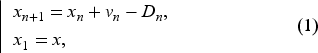
We study an infinite horizon inventory problem in which the inventory manager (IM) does not fully know the demand’s probability density function (PDF). We write this density as $g(z|\xi )$ with $\xi$ , a parameter unknown to the IM. We allow backlogging so the IM can learn about $\xi$ by observing realized demands over time. We let $G(z|\xi )$ denote the cumulative distribution function (CDF), $G(z|\xi )={\int }_0^{z}g(t|\xi )dt$ and complementary CDF (CCDF), $\overline{G}(z|\xi )=1-G(z|\xi ).$ Since the information comes from observing demands, we introduce the filtration ${\mathcal{D}}^n=\sigma (D_1,\dots ,D_n),n\ge 1.$ The order quantity $v_n$ in period $n$ is adapted to ${\mathcal{D}}^{n-1}$ . At the beginning of period 1, the given inventory $x_1=x$ , the IM has no information except an initial belief about $\xi ,$ expressed by the PDF $f(\xi )$ on $\mathbb{R}.$ From the inventory evolution equation,

$$|\begin{array}{c}\begin{array}{rl}& x_{n+1}=x_n+v_n-D_n,\\ & x_1=x,\end{array}\end{array}$$

(1)

we see that the inventory process $x_n$ is also adapted to ${\mathcal{D}}^{n-1}$ .

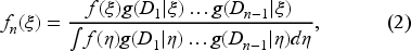
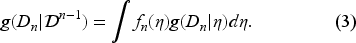
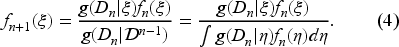
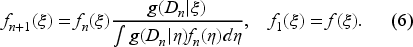
The updated belief $f_n(\xi )$ after observing the demands $D_1,\dots ,D_{n-1}$ can be written as follows:

$$f_n(\xi )={\displaystyle \frac{f(\xi )g(D_1|\xi )\dots g(D_{n-1}|\xi )}{\int f(\eta )g(D_1|\eta )\dots g(D_{n-1}|\eta )d\eta }},$$

(2)

because the numerator gives the joint probability density of $\xi ,D_1,\dots ,D_{n-1},$ since the demands are independent given the parameter $\xi ,$ and the denominator is the joint probability density of the demands as they are no longer independent in the presence of the parameter. We use $f_n(\xi )$ to obtain the conditional density of $D_n$ , given $D_1,\dots ,D_{n-1}$ , as

$$g(D_n|{\mathcal{D}}^{n-1})=\int f_n(\eta )g(D_n|\eta )d\eta .$$

(3)

We use Bayes’ theorem to obtain

$$f_{n+1}(\xi )={\displaystyle \frac{g(D_n|\xi )f_n(\xi )}{g(D_n|{\mathcal{D}}^{n-1})}}={\displaystyle \frac{g(D_n|\xi )f_n(\xi )}{\int g(D_n|\eta )f_n(\eta )d\eta }}.$$

(4)

By setting $y_n=x_n+v_n$ , we write (1) and (4) as follows:

$$\begin{array}{rl}{x}_{n+1}& =y_n-D_n,x_1=x,\end{array}$$

(5)

$$\begin{array}{rl}{f}_{n+1}(\xi )& =f_n(\xi )\frac{g(D_n|\xi )}{\int g(D_n|\eta )f_n(\eta )d\eta },f_1(\xi )=f(\xi ).\end{array}$$

(6)

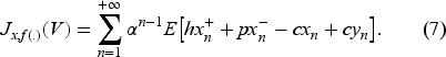
The state $(x_n,f_n(.))$ of our dynamic system is a stochastic process adapted to ${\mathcal{D}}^{n-1}$ with the state space $\mathbb{R}\times \mathcal{L}(\mathbb{R}),$ where $\mathcal{L}(\mathbb{R})$ is the set of probability densities on $\mathbb{R}.$ We can now define our inventory control problem. We set the decision $V=\{y_1,\dots ,y_n,\dots \}$ with $y_1=y\ge x,$ $y_n\ge x_n,$ where $y_n-x_n$ denotes the order quantity in period $n.$ Let $x_n^{+}=max(0,x_n)$ and $x_n^{-}=max(0,-x_n)$ represent the inventory and the backlog in period $n,$ respectively. Let $p,$ $h,$ and $c$ denote the backlog cost per unit per period, inventory holding cost per unit per period, and unit ordering cost, respectively. Let $\alpha$ be the discount factor. Then, the expected total cost is

$$J_{x,f(.)}(V)=\sum _{n=1}^{+\mathrm{\infty }}{\alpha }^{n-1}E[h{x}_n^{+}+p{x}_n^{-}-c{x}_n+c{y}_n].$$

(7)

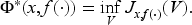
We define the value function as follows:

$$\mathrm{\Phi }(x,f(.))=\underset{V}{inf}{J}_{x,f(.)}(V),$$

(8)

where $(x,f(.))$ is the initial system state.

4. Dynamic Programming and Required Bounds

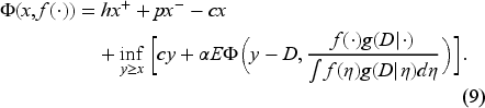
We use dynamic programming to write the functional Bellman equation for the value function $\mathrm{\Phi }(x,f(.)):$

$$\begin{array}{rl}\mathrm{\Phi }(x,f(\cdot ))& =h{x}^{+}+p{x}^{-}-cx\\ & +\underset{y\ge x}{inf}[cy+\alpha E\mathrm{\Phi }(y-D,\frac{f(\cdot )g(D|\cdot )}{\int f(\eta )g(D|\eta )d\eta })].\end{array}$$

(9)

As the Bellman equation may have many solutions, we develop the conditions under which the value function becomes its unique solution. In Subsection 4.1, we obtain lower and upper bounds on the value function, allowing us, as in Section 5, to show that the solution of the Bellman equation is unique when restricted to these bounds and is, indeed, the value function. Furthermore, we can use these bounds also to obtain an upper bound on the order-up-to-level decision $y$ . Note that the initial inventory level $x$ is naturally a lower bound on $y$ . These decision bounds allow us to obtain a modified Bellman equation, which, together with an intermediate comparison result obtained in Subsection 4.2, help us prove the uniqueness of the Bellman equation solution and the existence of an optimal state-dependent policy in Section 5.

4.1. Bounds on Value Function and Decision

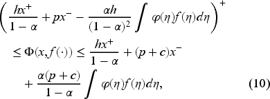
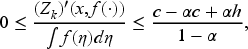
Lemma 1 below gives the bounds on the value function (derived in EC.3.1 in the E-Companion) sufficient to ensure it is the unique solution to the Bellman equation (9).

Lemma 1

The value function $\mathrm{\Phi }(x,f(\cdot ))$ defined in (8) satisfies

$$\begin{array}{rl}& {(\frac{h{x}^{+}}{1-\alpha }+p{x}^{-}-\frac{\alpha h}{(1-\alpha {)}^2}\int \phi (\eta )f(\eta )d\eta )}^{+}\\ & \le \mathrm{\Phi }(x,f(\cdot ))\le \frac{h{x}^{+}}{1-\alpha }+(p+c)x^{-}\\ & +\frac{\alpha (p+c)}{1-\alpha }\int \phi (\eta )f(\eta )d\eta ,\end{array}$$

(10)

where $\int \phi (\eta )f(\eta )d\eta <+\mathrm{\infty }$ , with

$$\phi (\eta )={\int }_0^{+\mathrm{\infty }}\overline{G}(z|\eta )dz.$$

(11)

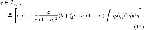
These bounds also provide an upper limit for the order-up-to-level decision $y$ . Furthermore, given that $y\ge x$ by definition, we establish the following admissibility interval for $y$ in EC.3.2 in the E-Companion:

$$\begin{array}{rl}& y\in {\mathcal{I}}_{x,f(\cdot )}\\ & \triangleq [x,x^{+}+\frac{1}{c}\frac{\alpha }{(1-\alpha {)}^2}(h+(p+c)(1-\alpha ))\int \phi (\eta )f(\eta )d\eta ].\end{array}$$

(12)

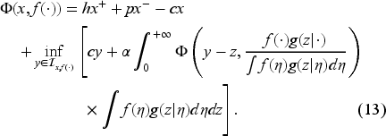
We replace the domain $y\ge x$ in (9) with the interval (12) to obtain the modified Bellman equation

$$\begin{array}{rl}& \mathrm{\Phi }(x,f(\cdot ))=h{x}^{+}+p{x}^{-}-cx\\ & +\underset{y\in {\mathcal{I}}_{x,f(\cdot )}}{inf}[cy+\alpha {\int }_0^{+\mathrm{\infty }}\mathrm{\Phi }(y-z,\frac{f(\cdot )g(z|\cdot )}{\int f(\eta )g(z|\eta )d\eta })\\ & \times \int f(\eta )g(z|\eta )d\eta dz].\end{array}$$

(13)

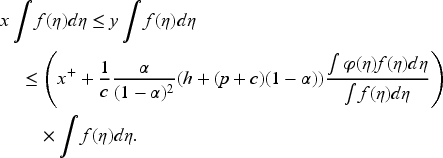
In Subsection 5.1, we transform (13) into its unnormalized counterpart (22) and the interval (12) into (19). This compact admissibility interval aids in determining the state-dependent policy. Specifically, the right-hand side in equation (22) is continuous in $y$ and thus achieves its minimum at $\hat{y}$ in the compact admissibility interval. In Subsection 5.2, we show that the unique solution of (13) and (12) is the value function.

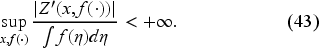
4.2. Comparison of Value Function With Solutions of Bellman Equation

We present a significant comparison result between any solution of (13), satisfying the bounds in (10), and the value function $\underset{V}{inf}{J}_{x,f(\cdot )}(V)$ defined in (8). For clarity, we temporarily denote the value function as follows:

$${\mathrm{\Phi }}^{*}(x,f(\cdot ))=\underset{V}{inf}{J}_{x,f(\cdot )}(V).$$

Lemma 2

Any solution $\mathrm{\Phi }(x,f(\cdot ))$ of the functional equation (13) honoring (10) holding satisfies

$$\mathrm{\Phi }(x,f(\cdot ))\le {\mathrm{\Phi }}^{*}(x,f(\cdot ))=\underset{V}{inf}{J}_{x,f(\cdot )}(V).$$

(14)

This result (proved in EC.4.1 in the E-Companion) will be required to establish a central result in the next section.

5. Uniqueness of Solution of Bellman Equation and Existence of Optimal Policy

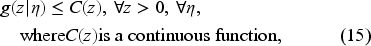
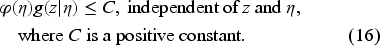
We prove that the value function is the unique solution of the Bellman equation and that an optimal state-dependent policy exists. We make the following assumptions:

$$\begin{array}{rl}& g(z|\eta )\le C(z),\mathrm{\forall }z>0,\mathrm{\forall }\eta ,\\ & \text{where}C(z)\text{is a continuous function,}\end{array}$$

(15)

$$\begin{array}{rl}& \phi (\eta )g(z|\eta )\le C,\text{independent of}z\text{and}\eta ,\\ & \text{where}C\text{is a positive constant.}\end{array}$$

(16)

We provide their rationale at the end of Subsection 5.1. These assumptions will remain in force in this section and Section 6, and they are satisfied in the particular cases treated in Sections 7 and 8.

Theorem 1

For any probability density $f(.)$ on $\mathbb{R}$ such that $\int \phi (\eta )f(\eta )d\eta <+\mathrm{\infty },$ the value function $\mathrm{\Phi }(x,f(.))$ is the unique functional such that (10) and (13) hold. Moreover, there exists a $\hat{y}(x,f(.))$ that attains the inf in (13).

For its proof, it is convenient to work with unnormalized probability, now a standard trick making the belief updating (13) linear and facilitating our study of the Bellman equation in Subsections 5.1 and 5.2.

5.1. Unnormalized Bellman Equation

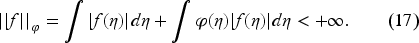
Consider the space of functions on $\mathbb{R}$ such that

$$||f|{|}_{\phi }=\int |f(\eta )|d\eta +\int \phi (\eta )|f(\eta )|d\eta <+\mathrm{\infty }.$$

(17)

This space is denoted as $L_{\phi }^1(\mathbb{R})$ , a Banach space for the norm $||f|{|}_{\phi }$ , as shown in EC.4.2 in the E-Companion. The subset of positive functions denoted by $L_{\phi +}^1(\mathbb{R})$ is closed.

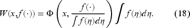
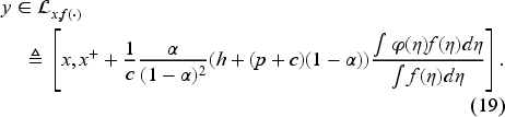
We introduce the unnormalized Bellman equation by extending the domain of $f(\cdot )$ to unnormalized probabilities, which include positive integrable functions encompassing probability densities. Thus, a functional on $\mathbb{R}$ and probability densities extends to a functional on $\mathbb{R}\times L_{\phi +}^1(\mathbb{R})$ via the formula

$$W(x,f(\cdot ))=\mathrm{\Phi }(x,\frac{f(\cdot )}{\int f(\eta )d\eta })\int f(\eta )d\eta .$$

(18)

Note that $W(x,f(\cdot ))$ and $\mathrm{\Phi }(x,f(\cdot ))$ coincide when $f(\cdot )$ is a probability density.

From (12) and (18), it is evident that the decision $y$ satisfies

$$\begin{array}{rl}& x\int f(\eta )d\eta \le y\int f(\eta )d\eta \\ & \le (x^{+}+\frac{1}{c}\frac{\alpha }{(1-\alpha {)}^2}(h+(p+c)(1-\alpha ))\frac{\int \phi (\eta )f(\eta )d\eta }{\int f(\eta )d\eta })\\ & \times \int f(\eta )d\eta .\end{array}$$

Hence, we define

$$\begin{array}{rl}& y\in {\mathcal{L}}_{x,f(\cdot )}\\ & \triangleq [x,x^{+}+\frac{1}{c}\frac{\alpha }{(1-\alpha {)}^2}(h+(p+c)(1-\alpha ))\frac{\int \phi (\eta )f(\eta )d\eta }{\int f(\eta )d\eta }].\end{array}$$

(19)

Also, from (18), we have

$$W(x,\mu f(\cdot ))=\mu W(x,f(\cdot )),\mathrm{\forall }\mu >0,$$

(20)

leading to

$$\begin{array}{rl}W(y-z,f(\cdot )g(z|\cdot ))& =\mathrm{\Phi }(y-z,\frac{f(\cdot )g(z|\cdot )}{\int f(\eta )g(z|\eta )d\eta })\\ & \times \int f(\eta )g(z|\eta )d\eta .\end{array}$$

(21)

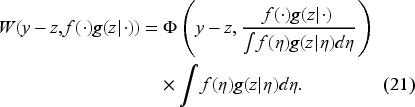
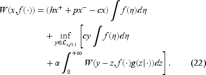
Thus, combining (13), (18), and (21), we obtain the unnormalized Bellman equation

$$\begin{array}{rl}W(x,f(\cdot ))& =(h{x}^{+}+p{x}^{-}-cx)\int f(\eta )d\eta \\ & +\underset{y\in {\mathcal{L}}_{x,f(\cdot )}}{inf}[cy\int f(\eta )d\eta \\ & +\alpha {\int }_0^{+\mathrm{\infty }}W(y-z,f(\cdot )g(z|\cdot ))dz].\end{array}$$

(22)

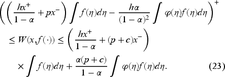
Furthermore, utilizing Lemma 1, we can readily derive the following bounds on $W(x,f(\cdot ))$

$$\begin{array}{rl}& {((\frac{h{x}^{+}}{1-\alpha }+p{x}^{-})\int f(\eta )d\eta -\frac{h\alpha }{(1-\alpha {)}^2}\int \phi (\eta )f(\eta )d\eta )}^{+}\\ & \le W(x,f(\cdot ))\le (\frac{h{x}^{+}}{1-\alpha }+(p+c)x^{-})\\ & \times \int f(\eta )d\eta +\frac{\alpha (p+c)}{1-\alpha }\int \phi (\eta )f(\eta )d\eta .\end{array}$$

(23)

Before proceeding to prove Theorem 1, it is worth noting that a solution of (22) and (23) satisfies (20). Also, (22) and (23) are equivalent to (13) and (10), respectively, and the optimal state-dependent policy, if it exists, remains identical for both Bellman equations. However, due to the simpler nature of (22) and the linearity in updating $f(\cdot )$ , we choose to work with (22) and (23). Finally, we provide the rationale for assumptions (15)-(16): the former ensures the well-definedness of $W(y-z,f(\cdot )g(z|\cdot ))$ , and the latter guarantees the integrability of $W(y_n-z,f_n(\cdot )g(z|\cdot ))$ in $z$ , allowing us to employ Lebesgue’s dominated convergence theorem.

5.2. Steps in Proof of Theorem 1

We base our proof on a monotonicity argument, a classical tool for variational inequalities, quasi-variational inequalities, and Bellman equations. Here, we list the five main steps in the proof and give the complete proof in EC.5 in the E-Companion.

Step 1.

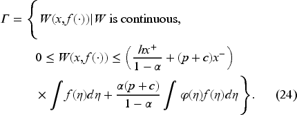
Since $W(x,f(\cdot ))$ must be positive, instead of requiring the sharper constraint on the left of (23), we only need to consider the set $\Gamma$ of functionals on $\mathbb{R}\times L_{\phi +}^1(\mathbb{R})$ such that

$$\begin{array}{rl}\Gamma & =\{W(x,f(\cdot ))|W\text{is continuous,}\\ & 0\le W(x,f(\cdot ))\le (\frac{h{x}^{+}}{1-\alpha }+(p+c)x^{-})\\ & \times \int f(\eta )d\eta +\frac{\alpha (p+c)}{1-\alpha }\int \phi (\eta )f(\eta )d\eta \}.\end{array}$$

(24)

Step 2.

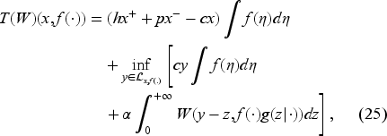
We define a monotone nonlinear operator $T$ on $\Gamma$ as

$$\begin{array}{rl}T(W)(x,f(\cdot ))& =(h{x}^{+}+p{x}^{-}-cx)\int f(\eta )d\eta \\ & +\underset{y\in {\mathcal{L}}_{x,f(.)}}{inf}[cy\int f(\eta )d\eta \\ & +\alpha {\int }_0^{+\mathrm{\infty }}W(y-z,f(\cdot )g(z|\cdot ))dz],\end{array}$$

(25)

and show that the operator $T$ maps $\Gamma$ into itself.

Step 3.

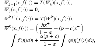
For the existence of a solution to (22), note that it is a fixed-point equation. Then, the functional $W(x,f(\cdot ))$ must satisfy $W(x,f(\cdot ))=T(W)(x,f(\cdot ))$ . We define two monotone sequences:

$$\begin{array}{rl}& |\begin{array}{c}\begin{array}{rl}& W_{k+1}(x,f(\cdot ))=T(W_k)(x,f(\cdot )),\\ & W_0(x,f(\cdot ))=0,\end{array}\end{array}\\ & |\begin{array}{c}\begin{array}{rl}& W^{k+1}(x,f(\cdot ))=T(W^k)(x,f(\cdot )),\\ & W^0(x,f(\cdot ))=(\frac{h{x}^{+}}{1-\alpha }+(p+c)x^{-})\\ & \int f(\eta )d\eta +\frac{\alpha (p+c)}{1-\alpha }\int \phi (\eta )f(\eta )d\eta ,\end{array}\end{array}\end{array}$$

and show that $W_k(x,f(\cdot ))$ is lower semi-continuous, converging to a lower semi-continuous function $\underset{\_}{W}(x,f(\cdot ))$ , and $W^k(x,f(\cdot ))$ is upper semi-continuous, converging to an upper semi-continuous function $\overline{W}(x,f(\cdot ))$ . Indeed, $\underset{\_}{W}(x,f(\cdot ))$ is the smallest solution, $\overline{W}(x,f(\cdot ))$ is the largest solution, and if $W(x,f(\cdot ))$ is any solution of (22), then we necessarily have

$$\underset{\_}{W}(x,f(\cdot ))\le W(x,f(\cdot ))\le \overline{W}(x,f(\cdot )).$$

(26)

Step 4.

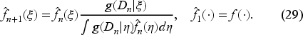
For the uniqueness of the solution, we revert to functions $f(\cdot )$ , which are probability densities. We can transfer the results in $W$ to results in $\mathrm{\Phi }$ and thus obtain the minimum and the maximum solutions $\underset{\_}{\mathrm{\Phi }}(x,f(\cdot ))$ and $\overline{\mathrm{\Phi }}(x,f(\cdot ))$ of (13). Thanks to the feedback $\hat{y}(x,f(\cdot ))$ given by the selection theorem, we construct the processes ${\hat{x}}_n$ , ${\hat{y}}_n,$ and ${\hat{f}}_n(\cdot )$ by the iterations

$$\begin{array}{rl}{\hat{y}}_n& =\hat{y}({\hat{x}}_n,{\hat{f}}_n(\cdot )),\end{array}$$

(27)

$$\begin{array}{rl}{\hat{x}}_{n+1}& ={\hat{y}}_n-D_n,{\hat{x}}_1=x,\end{array}$$

(28)

$$\begin{array}{rl}{\hat{f}}_{n+1}(\xi )& ={\hat{f}}_n(\xi )\frac{g(D_n|\xi )}{\int g(D_n|\eta ){\hat{f}}_n(\eta )d\eta },{\hat{f}}_1(\cdot )=f(\cdot ).\end{array}$$

(29)

We show that the minimum solution coincides with the value function by first setting $\hat{V}=({\hat{y}}_1,\dots ,{\hat{y}}_n,\dots )$ and showing that

$$\underset{\_}{\mathrm{\Phi }}(x,f(\cdot ))\ge J_{x,f(\cdot )}(\hat{V})\ge {\mathrm{\Phi }}^{*}(x,f(\cdot ))=\underset{V}{inf}{J}_{x,f(\cdot )}(V).$$

Since $\underset{\_}{\mathrm{\Phi }}(x,f(\cdot ))$ is the smallest solution, all solutions are larger than the value function. On the other hand, by Lemma 2, all solutions are smaller than the value function. Necessarily, the solution is unique and coincides with the value function.

Step 5.

Finally, the feedback $\hat{y}(x,f(\cdot ))$ allows us to construct an optimal control by using (27) to (29). The following section proves that this feedback is a base-stock policy.

Our proof diverges significantly from previous works on partially observable inventory control problems, such as Bensoussan et al. (2007, 2008a, 2008b, 2009) and Bensoussan and Guo (2015), despite some shared aspects, such as the utilization of unnormalized Bellman equations. Moreover, our value function has the inventory state and not just the probability density state, as in the value functions in the papers mentioned above. According to Bensoussan et al. (2007) and Bensoussan et al. (2009), the uniqueness of the solution is established through contraction mapping, although there are similarities in establishing the solution’s continuity. Meanwhile, Bensoussan et al. (2008a) employ induction arguments but omit monotonicity arguments. According to Bensoussan et al. (2008b), the uniqueness and continuity of the solution to dynamic programming equations are proved under certain conditions, allowing the use of Banach’s fixed-point theorem to establish the existence and uniqueness of the solution to the optimality equation directly, along with the value iteration algorithm. In contrast, Bensoussan and Guo (2015) also use the unnormalized Bellman equation and find that the optimal order-up-to level when stockout times are observable exceeds those when lost sales are observable.

Before proceeding to the next section, let us mention that $\mathrm{\Phi }(x,f(\cdot ))$ obtained in Theorem 1 is continuous from the facts that $\underset{\_}{\mathrm{\Phi }}(x,f(\cdot ))$ is l.s.c., $\overline{\mathrm{\Phi }}(x,f(\cdot ))$ is u.s.c., and $\underset{\_}{\mathrm{\Phi }}(x,f(\cdot ))=\overline{\mathrm{\Phi }}(x,f(\cdot ))=\mathrm{\Phi }(x,f(\cdot ))$ .

6. Optimality of Base-Stock Policy

When there is no unknown parameter, there is no learning, and the optimal feedback is a base-stock policy. When there is learning, the optimal policy is also a base-stock policy, with the base-stock level now depending on the current belief updated based on the realized past demands. Here, we obtain this result in a more general setting than in the literature.

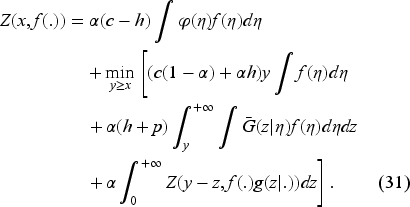
Instead of Bellman equation (22), it is convenient to consider an equivalent problem by setting

$$Z(x,f(.))=W(x,f(.))-(h{x}^{+}+p{x}^{-}-cx)\int f(\eta )d\eta .$$

(30)

Let us note that we do not need to impose the upper bound on $y$ to minimize the right-hand side of (30), as it will be automatically satisfied at a minimum point. We can write the Bellman equation for $Z(x,f(\cdot ))$ as follows:

$$\begin{array}{rl}Z(x,f(.))& =\alpha (c-h)\int \phi (\eta )f(\eta )d\eta \\ & +\underset{y\ge x}{min}[(c(1-\alpha )+\alpha h)y\int f(\eta )d\eta \\ & +\alpha (h+p){\int }_y^{+\mathrm{\infty }}\int \overline{G}(z|\eta )f(\eta )d\eta dz\\ & +\alpha {\int }_0^{+\mathrm{\infty }}Z(y-z,f(.)g(z|.))dz].\end{array}$$

(31)

The details of the transformation from (22) to (31) are in EC.6.1 in the E-Companion. The advantage of this formulation is that $x$ appears only in the constraint on $y$ . We know from Theorem 1 that this equation has a unique continuous solution in the following interval:

$$\begin{array}{rl}& Z_0(x,f(.))\\ & \triangleq ({\displaystyle \frac{\alpha h{x}^{+}}{1-\alpha }}+cx)\int f(\eta )d\eta -{\displaystyle \frac{\alpha h}{(1-\alpha {)}^2}}\int \phi (\eta )f(\eta )d\eta \\ & \le Z(x,f.))\le Z^0(x,f(.))\triangleq ({\displaystyle \frac{\alpha h}{1-\alpha }}+c)x^{+}\\ & \times \int f(\eta )d\eta +{\displaystyle \frac{\alpha (p+c)}{1-\alpha }}\int \phi (\eta )f(\eta )d\eta .\end{array}$$

(32)

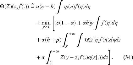
The solution of (31) is a fixed point of the operator

$$Z(x,f(.))=\mathrm{\Theta }(Z)(x,f(.))$$

(33)

with

$$\begin{array}{rl}\mathrm{\Theta }(Z)(x,f(.))& \triangleq \alpha (c-h)\int \phi (\eta )f(\eta )d\eta \\ & +\underset{y\ge x}{min}[(c(1-\alpha )+\alpha h)y\int f(\eta )d\eta \\ & +\alpha (h+p){\int }_y^{+\mathrm{\infty }}\int \overline{G}(z|\eta )f(\eta )d\eta dz\\ & +\alpha {\int }_0^{+\mathrm{\infty }}Z(y-z,f(.)g(z|.))dz].\end{array}$$

(34)

It is a nonlinear operator on functionals $Z(x,f(.))$ defined on $\mathbb{R}\times L_{\phi +}^1(\mathbb{R})$ and satisfying the bounds in (32).

6.1. Preserving Convexity

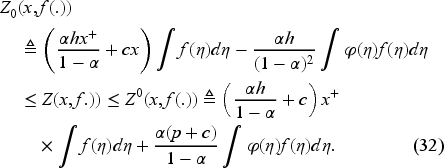
The following property (proved in EC.6.2 in the E-Companion) aids us in establishing the convexity required to demonstrate the optimality of a base-stock policy.

Proposition 1

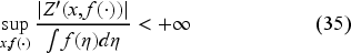
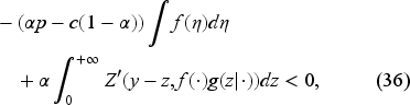
Suppose the function $Z(x,f(\cdot ))$ is continuously differentiable, increasing, and convex in $x$ . Assume that

$$\underset{x,f(\cdot )}{sup}{\displaystyle \frac{|Z^{\prime }(x,f(\cdot ))|}{\int f(\eta )d\eta }}<+\mathrm{\infty }$$

(35)

and

$$\begin{array}{rl}& -(\alpha p-c(1-\alpha ))\int f(\eta )d\eta \\ & +\alpha {\int }_0^{+\mathrm{\infty }}{Z}^{\prime }(y-z,f(\cdot )g(z|\cdot ))dz<0,\end{array}$$

(36)

where $Z^{\prime }(x,f(\cdot ))$ is the derivative of $Z(x,f(\cdot ))$ with respect to $x$ . Then, $x\to \mathrm{\Theta }(Z)(x,f(\cdot ))$ and $x\to Z(x,f(\cdot ))$ have the same properties.

Assumption (35) ensures that the norm of the specified derivative of the operator is well-defined. Equation (36) is required to demonstrate that the function, dependent on the order-up-to-level decision $y$ , has a root.

6.2. Base-Stock Policy

We now show the optimal policy as a base-stock policy.

Theorem 2

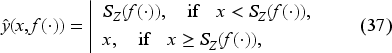
$Z(x,f(\cdot ))$ is continuously differentiable, increasing, and convex in $x$ . The optimal policy is

$$\hat{y}(x,f(\cdot ))=|\begin{array}{c}\begin{array}{rl}& S_Z(f(\cdot )),\text{if}x<S_Z(f(\cdot )),\\ & x,\text{if}x\ge S_Z(f(\cdot )),\end{array}\end{array}$$

(37)

where $S_Z(f(\cdot ))$ is the base-stock level depending only on the current belief $f(\cdot )$ .

Proof.

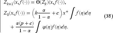
We consider the increasing sequence

$$|\begin{array}{c}\begin{array}{rl}& Z_{k+1}(x,f(\cdot ))=\mathrm{\Theta }(Z_k)(x,f(\cdot )),\\ & Z_0(x,f(\cdot ))=(h{\displaystyle \frac{\alpha }{1-\alpha }}+c)x^{+}\int f(\eta )d\eta \\ & +{\displaystyle \frac{\alpha (p+c)}{1-\alpha }}\int \phi (\eta )f(\eta )d\eta .\end{array}\end{array}$$

(38)

Note that the function $Z_0(x,f(\cdot ))$ is continuously differentiable in $x$ except at $x=0,$ and it satisfies (35) and (36). Note also that $Z(x,f(\cdot ))$ appears inside an integral in (34), and $\mathrm{\Theta }(Z)(x,f(\cdot ))$ is constant for $x<S_Z(f(\cdot )).$ Thus, by way of (38), the operator $\mathrm{\Theta }(Z)(x,f(\cdot ))$ transforms $Z_0(x,f(\cdot ))$ into a continuously differentiable function. Then, by the stability properties of Proposition 1, we get sequentially the same properties for $Z_k(x,f(\cdot )),$ $k\ge 1,$ and consequently for the limit $Z(x,f(\cdot ))$ . Also, we can check sequentially that

$$0\le {\displaystyle \frac{(Z_k{)}^{\prime }(x,f(\cdot ))}{\int f(\eta )d\eta }}\le {\displaystyle \frac{c-\alpha c+\alpha h}{1-\alpha }},$$

which carries to the limit

$$0\le {\displaystyle \frac{Z^{\prime }(x,f(\cdot ))}{\int f(\eta )d\eta }}\le {\displaystyle \frac{c-\alpha c+\alpha h}{1-\alpha }}.$$

(39)

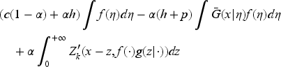
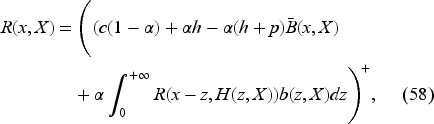
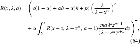
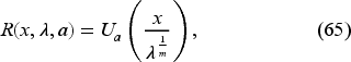
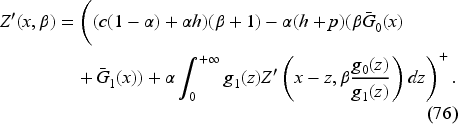
The optimal feedback is then the base-stock policy (37) with the base-stock level $S_Z(f(\cdot ))$ as the unique solution of $Q{(Z)}^{\prime }(S_Z(f(\cdot )),f(\cdot ))=0,$ where $Q{(Z)}^{\prime }(y,f(\cdot ))$ is the derivative of expression inside the min operation on the right-hand side in (34) with respect to $y$ . In EC.6.2 in the E-Companion, we show it to be given by the following equation:

$$\begin{array}{rl}& Q{(Z)}^{\prime }(y,f(\cdot ))\\ & =(c(1-\alpha )\\ & +\alpha h)\int f(\eta )d\eta -\alpha (h+p)\int \overline{G}(y|\eta )f(\eta )d\eta \\ & +\alpha {\int }_0^{+\mathrm{\infty }}{Z}^{\prime }(y-z,f(\cdot )g(z|\cdot ))dz.◼\end{array}$$

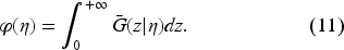
6.3. Obtaining the Base-Stock Level

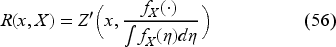
We define

$$S_Z(f(\cdot ))=sup\{x|Z^{\mathrm{\prime }}(x,f(\cdot ))=0\}.$$

(40)

Thus, to obtain the base-stock level, we do not need to obtain $Z(x,f(\cdot ))$ if we could find $Z^{\mathrm{\prime }}(x,f(\cdot ))$ directly. Indeed, we have

$$\begin{array}{rl}& Z^{\mathrm{\prime }}(x,f(\cdot ))\\ & =|\begin{array}{c}\begin{array}{rl}& 0,\text{if}x<S_Z(f(\cdot )),\\ \\ & (c(1-\alpha )+\alpha h)\int f(\eta )d\eta -\alpha (h+p)\int \overline{G}(x|\eta )f(\eta )d\eta \\ & +\alpha {\int }_0^{+\mathrm{\infty }}{Z}^{\prime }(x-z,f(\cdot )g(z|\cdot ))dz,\text{if}x\ge S_Z(f(\cdot )).\end{array}\end{array}\end{array}$$

(41)

Since the second expression is positive, $Z^{\mathrm{\prime }}(x,f(\cdot ))$ satisfies

$$\begin{array}{rl}{Z}^{\mathrm{\prime }}(x,f(\cdot ))& =((c(1-\alpha )+\alpha h)\int f(\eta )d\eta \\ & -\alpha (h+p)\int \overline{G}(x|\eta )f(\eta )d\eta \\ & {+\alpha {\int }_0^{+\mathrm{\infty }}{Z}^{\prime }(x-z,f(\cdot )g(z|\cdot ))dz)}^{+}.\end{array}$$

(42)

The following property (proved in EC.6.3 in the E-Companion) demonstrates that (42) has a unique solution $Z^{\mathrm{\prime }}(x,f(\cdot ))$ . Furthermore, we can recover the value function $Z(x,f(\cdot ))$ if needed.

Proposition 2

Equation (42) has one and only one solution in the functional space of continuous functions on $\mathbb{R}\times L_{\phi +}^1(\mathbb{R})$ with the norm

$$\underset{x,f(\cdot )}{sup}{\displaystyle \frac{|Z^{\prime }(x,f(\cdot ))|}{\int f(\eta )d\eta }}<+\mathrm{\infty }.$$

(43)

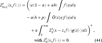
We introduce an algorithm for computing the base-stock level and obtain interesting properties of non-negativity, monotonicity, and convergence of the iterative sequence.

6.4. Monotonicity Properties

We consider the iterative sequence

$$\begin{array}{rl}{Z}_{k+1}^{\mathrm{\prime }}(x,f(\cdot ))& =((c(1-\alpha )+\alpha h)\int f(\eta )d\eta \\ & -\alpha (h+p)\int \overline{G}(x|\eta )f(\eta )d\eta \\ & {+\alpha {\int }_0^{+\mathrm{\infty }}{Z}_k^{\prime }(x-z,f(\cdot )g(z|\cdot ))dz)}^{+},\\ & \text{with}{Z}_0^{\mathrm{\prime }}(x,f(\cdot ))=0.\end{array}$$

(44)

By recurrence, we see that

$$Z_k^{\prime }(x,f(\cdot ))\ge 0\text{, and it is increasing in}x.$$

(45)

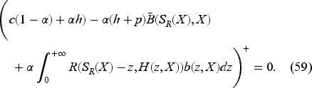
Consequently,

$$\begin{array}{rl}& (c(1-\alpha )+\alpha h)\int f(\eta )d\eta -\alpha (h+p)\int \overline{G}(x|\eta )f(\eta )d\eta \\ & +\alpha {\int }_0^{+\mathrm{\infty }}{Z}_k^{\prime }(x-z,f(\cdot )g(z|\cdot ))dz\end{array}$$

is increasing in $x.$ Since it reduces to $-(\alpha p-c(1-\alpha ))\int f(\eta )d\eta$ at $x=-\mathrm{\infty }$ and is larger than $(c(1-\alpha )+\alpha h)\int f(\eta )d\eta$ at $x=+\mathrm{\infty }$ , there exists a unique $S_{Z_{k+1}}(f(\cdot ))$ such that

$$Z_{k+1}^{\prime }(x,f(\cdot ))=0,\text{if}x\le S_{Z_{k+1}}(f(\cdot )).$$

(46)

Also, $Z_1^{\mathrm{\prime }}(x,f(\cdot ))\ge Z_0^{\mathrm{\prime }}(x,f(\cdot )).$ By recurrence again, we have

$$Z_{k+1}^{\prime }(x,f(\cdot ))\ge Z_k^{\prime }(x,f(\cdot )).$$

(47)

Since (42) is a fixed point of a contraction, we can assert that

$$Z_k^{\prime }(x,f(\cdot ))\uparrow Z^{\prime }(x,f(\cdot )).$$

(48)

From the definition of $S_{Z_k}(f(\cdot )),$ we immediately get a valuable monotonicity property regarding the base-stock level for any given belief, that is,

$$S_{Z_{k+1}}(f(\cdot ))\le S_{Z_k}(f(\cdot )).$$

(49)

Thus,

$$S_{Z_k}(f(\cdot ))\downarrow S_Z(f(\cdot )).$$

(50)

These monotonicity properties allow us to develop an iterative procedure to compute the optimal belief-dependent base-stock level $S_Z(f(\cdot ))$ for any given belief $f(\cdot )$ as the limit of a decreasing sequence of nonnegative numbers. We provide this procedure in EC.6.4 in the E-Companion. This procedure yields the stationary function $S_Z(f(\cdot ))$ , which we can use offline to obtain the optimal base-stock level in period $n$ once we have the updated belief $f_n(\cdot )$ in that period. Knowing the inventory and the base-stock level in that period, we can make the optimal ordering decision based on the order-up-to level according to (37). Then, we observe the demand in that period, allowing us to update the belief to $f_{n+1}(\cdot )$ and move to the next period $n+1$ , obtain the optimal base-stock level $S_{Z_{n+1}}(f(\cdot ))$ , and so on.

For computations in the case of a general infinite-dimensional belief, there will be a need to discretize the belief density to obtain this function for offline use. In Sections 7 and 8, we limit ourselves to parametric demand and belief densities so that the belief density is finite-dimensional, and we can obtain the function $S_Z(f(\cdot ))$ without discretization.

7. Learning With Conjugate Probabilities

Here, we focus on the case of conjugate probabilities discussed in much of the related literature, including Azoury (1985), Iglehart (1964), Scarf (1959), and Scarf (1960). They study only finite-horizon problems and analyze them via a sequence of functions. By contrast, we study stationary infinite-horizon problems and do not need their setup as we treat them as particular cases of our general theory.

In Subsection 7.1, we specialize the belief function $f(\cdot )$ introduced in our general approach to depend on a vector $X$ of hyperparameters, writing it as $f_X(\xi )$ . We then show that the general problem gives the hyperparameter vector $X$ as a sufficient statistic and provides an equation to be satisfied by the base-stock level expressed as a function of $X$ . Since we settle the existence and uniqueness issues in a general setting, our results transfer the settlement of these issues to the cases treated in this section.

In Subsection 7.2, we consider particular cases of Weibull demand whose scale parameter is unknown. So, we choose our belief function from its conjugate-prior family of gamma densities, characterized by two hyperparameters. We obtain the optimal base-stock level as a function of the two gamma hyperparameters; see EC.7.1 in the E-Companion for details. We also present two numerical examples by generating demands for five periods according to supposedly true exponential and Weibull densities in Subsections 7.2.1 and 7.2.2, respectively. We obtain the sequence of optimal base-stock levels learned from these demands, order accordingly, and evolve the inventory dynamics. We also generate demands for one thousand periods and see the sequence of base-stock levels tending to converge to the asymptotic base-stock level in each example.

In Subsection 7.3, we compute base-stock levels using two myopic policies for the exponential example treated in Subsection 7.2.1. We then highlight the extent of their suboptimality by comparing their costs to the optimal cost. Due to space limitations, we omit this comparison for the examples in Subsection 7.2.2 and Section 8.

We define the demand’s probability density given $X$ as follows:

$$b(z,X)={\displaystyle \frac{\int f_X(\eta )g(z|\eta )d\eta }{\int f_X(\eta )d\eta }}.$$

(51)

We assume

$${\displaystyle \frac{f_X(\xi )g(z|\xi )}{\int f_X(\eta )d\eta }}=b(z,X){\displaystyle \frac{f_{H(z,X)}(\xi )}{\int f_{H(z,X)}(\eta )d\eta }},$$

(52)

which defines a coupling between the family $f_X(\xi )$ and the probability density $g(z|\xi )$ . Here, $H(z,X)$ is a vector of the same size as $X$ . These are the conjugate probabilities.

7.1. Sufficient Statistic

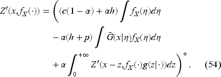
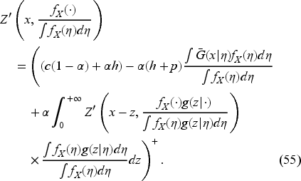
We want to study equation (42) for conjugate probabilities and see that the infinite-dimensional problem reduces to a problem of the dimension equaling the size of the vector $X$ of hyperparameters. We first note that $Z^{\mathrm{\prime }}(x,f(\cdot ))$ has the same property as $W(x,f(\cdot ))$ in (20), namely,

$$Z^{\mathrm{\prime }}(x,\mu f(\cdot ))=\mu Z^{\mathrm{\prime }}(x,f(\cdot )),\mathrm{\forall }\mu >0.$$

(53)

We write (42) as follows:

$$\begin{array}{rl}{Z}^{\mathrm{\prime }}(x,f_X(\cdot ))& =((c(1-\alpha )+\alpha h)\int f_X(\eta )d\eta \\ & -\alpha (h+p)\int \overline{G}(x|\eta )f_X(\eta )d\eta \\ & {+\alpha {\int }_0^{+\mathrm{\infty }}{Z}^{\mathrm{\prime }}(x-z,f_X(\cdot )g(z|\cdot ))dz)}^{+}.\end{array}$$

(54)

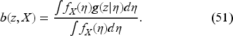
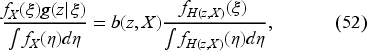
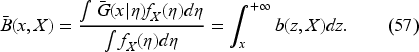
Using the property (53), we can write the following equation:

$$\begin{array}{rl}& Z^{\mathrm{\prime }}(x,{\displaystyle \frac{f_X(\cdot )}{\int f_X(\eta )d\eta }})\\ & =((c(1-\alpha )+\alpha h)-\alpha (h+p){\displaystyle \frac{\int \overline{G}(x|\eta )f_X(\eta )d\eta }{\int f_X(\eta )d\eta }}\\ & +\alpha {\int }_0^{+\mathrm{\infty }}{Z}^{\mathrm{\prime }}(x-z,{\displaystyle \frac{f_X(\cdot )g(z|\cdot )}{\int f_X(\eta )g(z|\eta )d\eta }})\\ & {\times {\displaystyle \frac{\int f_X(\eta )g(z|\eta )d\eta }{\int f_X(\eta )d\eta }}dz)}^{+}.\end{array}$$

(55)

Then we let

$$R(x,X)=Z^{\prime }(x,{\displaystyle \frac{f_X(\cdot )}{\int f_X(\eta )d\eta }})$$

(56)

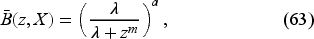
and the CCDF

$$\overline{B}(x,X)={\displaystyle \frac{\int \overline{G}(x|\eta )f_X(\eta )d\eta }{\int f_X(\eta )d\eta }}={\int }_x^{+\mathrm{\infty }}b(z,X)dz.$$

(57)

Importantly, because of (51) and (52), (55) becomes

$$\begin{array}{rl}R(x,X)& =((c(1-\alpha )+\alpha h-\alpha (h+p)\overline{B}(x,X)\\ & +\alpha {\int }_0^{+\mathrm{\infty }}R(x-z,H(z,X))b(z,X)dz{)}^{+},\end{array}$$

(58)

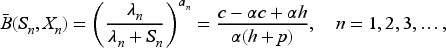
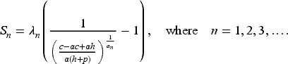
a finite-dimensional functional equation. It has one, and only one, solution on the set of bounded functions of $x$ and $X$ . We have $R(x,X)=0$ for $x\le 0$ , and there exists a single $S_R(X)>0$ such that $R(x,X)=0$ for $x\le S_R(X)$ . Moreover, $S_R(X)$ can be obtained as the unique solution of

$$\begin{array}{rl}& (c(1-\alpha )+\alpha h)-\alpha (h+p)\overline{B}(S_R(X),X)\\ & +\alpha {\int }_0^{+\mathrm{\infty }}R(S_R(X)-z,H(z,X))b(z,X)dz{)}^{+}=0.\end{array}$$

(59)

7.2. Weibull Demand and Computation of Optimal Base-Stock Level

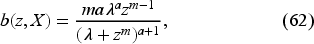
As a specific example, we consider the demand distributed according to the Weibull probability density

$$g(z|\xi )=m\xi z^{m-1}{e}^{-\xi z^m},$$

(60)

as by Azoury (1985) and Bensoussan (2011), where $m$ is the shape parameter, ${\xi }^{-1/m}$ is the scale parameter, and $\mathbb{E}(z^m)=1/\xi$ . As typical in the related literature, we assume that $m$ is known while $\xi$ is unknown. The mean demand is ${\xi }^{-1/m}\mathrm{\Gamma }(1+1/m)$ , where $\mathrm{\Gamma }(\cdot )$ is the gamma function. When $m=1$ , (60) reduces to the exponential density $\xi e^{-\xi z}$ with the mean demand $1/\xi$ .

For our belief on $\xi$ , we consider the unnormalized gamma family

$$f_X(\xi )={\xi }^{a-1}{e}^{-\lambda \xi },$$

(61)

with the hyperparameter $X=(\lambda ,a)$ , where $\lambda >0$ and $a>0$ are known as the rate and shape hyperparameters, respectively, in this shape-rate parametrization of the unnormalized gamma density. Moreover, $\int f_X(\eta )d\eta =\mathrm{\Gamma }(a)/{\lambda }^a$ , where $\mathrm{\Gamma }(a)$ stands for the gamma function defined as $\mathrm{\Gamma }(a)={\int }_0^{+\mathrm{\infty }}{x}^{a-1}{e}^{-x}dx.$ The standard version of the gamma density is ${\lambda }^a{f}_X(\xi )/\mathrm{\Gamma }(a)$ . In our context, $a$ denotes the current period, $\lambda$ denotes the cumulative $m$ th power of the observed demands, so $\lambda /a$ is the observed mean of the $m$ th power of the observed demands.

Substituting (60) and the conditional demand density

$$b(z,X)={\displaystyle \frac{ma{\lambda }^a{z}^{m-1}}{(\lambda +z^m{)}^{a+1}}},$$

(62)

as calculated in EC.7.1 in the E-Companion into (52), we see that (52) is satisfied with $H(z,X)=(\lambda +z^m,a+1)$ , that is, $f_{H(z,X)}(\xi )={\xi }^a{e}^{-(\lambda +z^m)\xi }$ .

Using (62) in equations (57) and (59), we have

$$\overline{B}(z,X)={\left(\frac{\lambda }{\lambda +z^m}\right)}^a,$$

(63)

the CCDF given the hyperparameter $X$ , and

$$\begin{array}{rl}R(x,\lambda ,a)& =(c(1-\alpha )+\alpha h-\alpha (h+p){\left(\frac{\lambda }{\lambda +x^m}\right)}^a\\ & +\alpha {\int }_0^{x}R(x-z,\lambda +z^m,a+1)\frac{ma{\lambda }^a{z}^{m-1}}{(\lambda +z^m{)}^{a+1}}dz{)}^{+},\end{array}$$

(64)

where $x>0$ . We rewrite

$$R(x,\lambda ,a)=U_a\left(\frac{x}{{\lambda }^{\frac{1}{m}}}\right),$$

(65)

where

$$\begin{array}{rl}{U}_a(x)& =(c(1-\alpha )+\alpha h-\alpha (h+p){\left(\frac{1}{1+x^m}\right)}^a\\ & +\alpha ma{\int }_0^x{U}_{a+1}\left(\frac{x-\zeta }{(1+{\zeta }^m{)}^{\frac{1}{m}}}\right)\frac{{\zeta }^{m-1}}{(1+{\zeta }^m{)}^{a+1}}d\zeta {)}^{+}.\end{array}$$

(66)

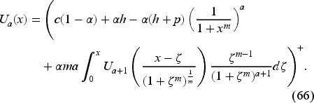
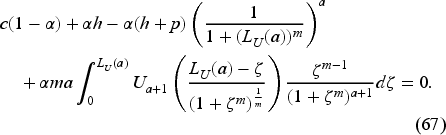
We have $U_a(x)=0$ for $x\le 0$ . We have thus reduced the dimensionality of the problem from $(x,\lambda ,a)$ to just $(x,a)$ and have obtained a simpler recursion (66), as is common in related literature. From (59), we see that the base-stock level $S_U(\lambda ,a)={\lambda }^{1/m}{L}_U(a)$ , where $L_U(a)$ is the solution of

$$\begin{array}{rl}& c(1-\alpha )+\alpha h-\alpha (h+p){\left(\frac{1}{1+(L_U(a){)}^m}\right)}^a\\ & +\alpha ma{\int }_0^{L_U(a)}{U}_{a+1}\left(\frac{L_U(a)-\zeta }{(1+{\zeta }^m{)}^{\frac{1}{m}}}\right)\frac{{\zeta }^{m-1}}{(1+{\zeta }^m{)}^{a+1}}d\zeta =0.\end{array}$$

(67)

The inventory manager can use equations (66) and (67) to compute in advance a surrogate base-stock level $L_U(a)$ for each period that depends only on the shape hyperparameter $a$ in that period and not on the scale (size) of the demand. Then, he can determine the optimal base-stock level ${\lambda }^{1/m}{L}_U(a)$ to use in each period by scaling the surrogate by the current best estimate of the demand, given by the scale hyperparameter consisting of the sum of the initial belief of the demand and the observed past demands. Each demand observation is raised to the power of $m$ to appropriately account for the characteristics of the Weibull distribution, which can exhibit skewness or heavy-tailed behavior, as governed by its shape parameter $m$ .

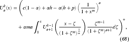
We approximate the solution of equation (66) by the recursive scheme

$$\begin{array}{rl}{U}_a^k(x)& =(c(1-\alpha )+\alpha h-\alpha (h+p){\left(\frac{1}{1+x^m}\right)}^a\\ & +\alpha ma{\int }_0^x{U}_{a+1}^{k-1}\left(\frac{x-\zeta }{(1+{\zeta }^m{)}^{\frac{1}{m}}}\right)\frac{{\zeta }^{m-1}}{(1+{\zeta }^m{)}^{a+1}}d\zeta {)}^{+},\end{array}$$

(68)

for $k=1,2,\dots ,$ with the initial guess $U_{a+1}^0(x)=0$ for all $a$ .

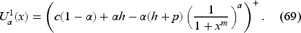
Here, we illustrate the iterative procedure to compute $U_a^k(x)$ for $k=1$ and $k=2$ only and provide a detailed description of the procedure in EC.7.2 in the E-Companion. Then, the solution $U_a(x)$ is given by $\underset{k\to \mathrm{\infty }}{lim}{U}_a^k(x)$ .

Set $k=1.$ Then,

$$U_a^1(x)={(c(1-\alpha )+\alpha h-\alpha (h+p){\left({\displaystyle \frac{1}{1+x^m}}\right)}^a)}^{+}.$$

(69)

For $k=2$ , the computation of $U_a^2(x)$ requires knowing $U_{a+1}^1(x)$ appearing inside the integral in (68). We obtain $U_{a+1}^1(x)$ by replacing $a$ with $a+1$ in (69). That gives

$$U_{a+1}^1(x)={(c(1-\alpha )+\alpha h-\alpha (h+p){\left({\displaystyle \frac{1}{1+x^m}}\right)}^{a+1})}^{+}.$$

(70)

We can then obtain

$$\begin{array}{rl}{U}_a^2(x)& =(c(1-\alpha )+\alpha h-\alpha (h+p){\left({\displaystyle \frac{1}{1+x^m}}\right)}^a\\ & {+\alpha ma{\int }_0^x{U}_{a+1}^1\left(\frac{x-\zeta }{(1+{\zeta }^m{)}^{\frac{1}{m}}}\right){\displaystyle \frac{{\zeta }^{m-1}}{(1+{\zeta }^m{)}^{a+1}}}d\zeta )}^{+}.\end{array}$$

(71)

We use the iterative procedure to solve two numerical examples given by the parameter values $\alpha =0.9$ , $p=4$ , $c=10$ , $h=1,$ and $m=1$ and $2$ .

7.2.1. Case $m=1$ , $g(z|\xi )=\xi e^{-\xi z}$

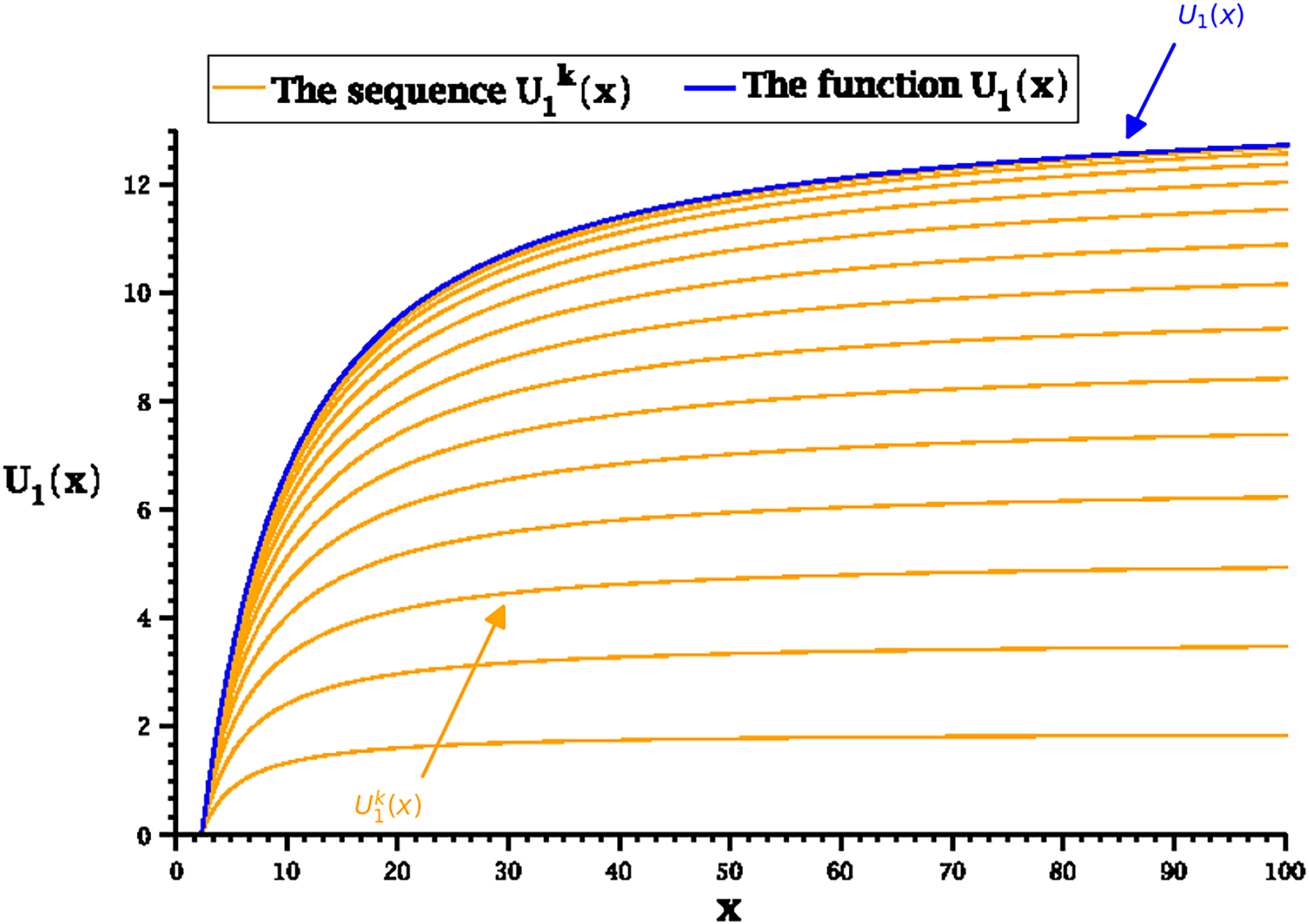
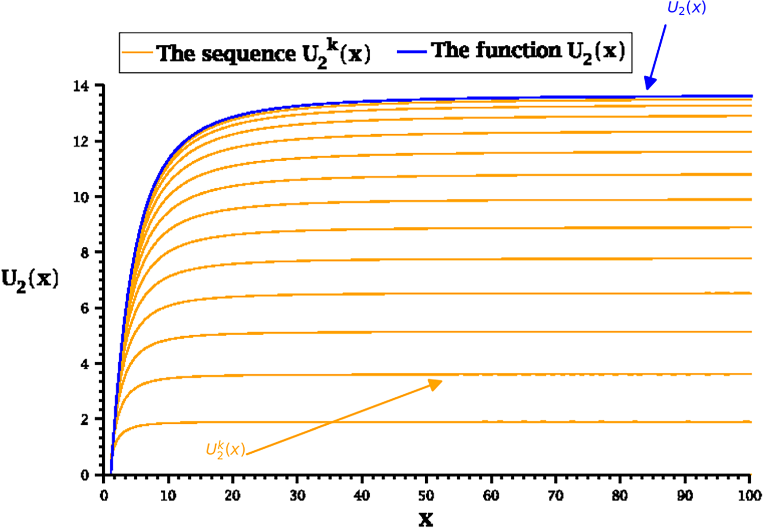
We compute $U_1(x),$ $U_2(x),\dots ,$ and $U_6(x),$ but display the results for only $U_1(x)$ and $U_2(x)$ in Figures 1 and 2, respectively.

Figure 1.

Convergence to the function $U_1(x)$ .

Figure 2.

Convergence to the function $U_2(x)$ .

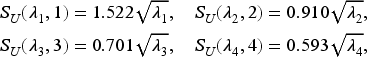
We use (67) to find $L_U(1)=2.316,$ $L_U(2)=7.324,$ $L_U(3)=0.493,$ $L_U(4)=0.351,$ and $L_U(5)=0.272$ , and formula $S_U(\lambda ,a)={\lambda }^{1/m}{L}_U(a)$ yields the base-stock levels $S_U({\lambda }_1,1)=2.316{\lambda }_1,$ $S_U({\lambda }_2,2)=0.778{\lambda }_2,$ $S_U({\lambda }_3,3)=0.493{\lambda }_3,$ $S_U({\lambda }_4,4)=0.351{\lambda }_4,$ and $S_U({\lambda }_5,5)=0.272{\lambda }_5.$

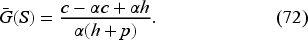
To illustrate how to implement our model, let us suppose the exponential demand (i.e., $m=1$ ) with $\xi =1/4$ . Thus, the mean demand is 4. We recall the base-stock level provided in EC.2 in the E-Companion as the unique solution of

$$\overline{G}(S)=\frac{c-\alpha c+\alpha h}{\alpha (h+p)}.$$

(72)

Then, the base-stock level using (72) is $S=3.448$ . However, the IM does not know this value and makes an initial guess of the hyperparameter $X$ . We will illustrate with three different guesses $X_1=({\lambda }_1,a_1)=(3,1)$ , $X_2=({\lambda }_1,a_1)=(5,1)$ , and $X_3=({\lambda }_1,a_1)=(10,1)$ , where ${\lambda }_1/a_1$ represents the initial mean of $\xi$ as 3, 5, and 10, respectively.

We use the predefined Matlab function $\mathtt{\text{exprnd}}(1/\xi ,1,N)$ to generate a sample path of $N=5$ demands from the exponential distribution with $\xi =1/4$ . These are $D_1=6.418,$ $D_2=0.409,$ $D_3=0.458,$ $D_4=3.895,$ and $D_5=\mathrm{5.542.}$

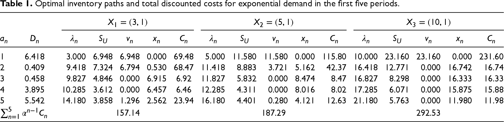
With our first guess of $X_1=(3,1)$ , we evolve the inventory using (1), starting with an initial $x_1=0$ . The base-stock level $S_U(3,1)=2.316{\lambda }_1=6.948$ , so we order the quantity $v_1=6.948$ . This results in $x_2=x_1+v_1-D_1=0.530$ . The cost for period 1 is calculated as $C_1=h{x}_1^{+}+p{x}_1^{-}+c{v}_1=\mathrm{69.48.}$ In period 2, the updated parameters are $({\lambda }_2,a_2)=({\lambda }_1+D_1,a_1+1)=(9.418,2)$ . The base-stock level is $S_U({\lambda }_2,a_2)=0.778{\lambda }_2=7.324$ . We then order $v_2=7.221$ , leading to $x_3=x_2+v_2-D_2=7.342,$ and $C_2=h{x}_2^{+}+p{x}_2^{-}+c{v}_2=\mathrm{72.74.}$ Following this process, we compute the inventory levels and costs for the first five periods. Similarly, we complete the dynamics corresponding to the initial guesses $X_2=(5,1)$ and $X_3=(10,1)$ . We summarize the results, including the total discounted costs, in Table 1.

Table 1.

Optimal inventory paths and total discounted costs for exponential demand in the first five periods.

		$X_1=(3,1)$					$X_2=(5,1)$					$X_3=(10,1)$
$a_n$	$D_n$	${\lambda }_n$	$S_U$	$v_n$	$x_n$	$C_n$	${\lambda }_n$	$S_U$	$v_n$	$x_n$	$C_n$	${\lambda }_n$	$S_U$	$v_n$	$x_n$	$C_n$
1	6.418	3.000	6.948	6.948	0.000	69.48	5.000	11.580	11.580	0.000	115.80	10.000	23.160	23.160	0.000	231.60
2	0.409	9.418	7.324	6.794	0.530	68.47	11.418	8.883	3.721	5.162	42.37	16.418	12.771	0.000	16.742	16.74
3	0.458	9.827	4.846	0.000	6.915	6.92	11.827	5.832	0.000	8.474	8.47	16.827	8.298	0.000	16.333	16.33
4	3.895	10.285	3.612	0.000	6.457	6.46	12.285	4.311	0.000	8.016	8.02	17.285	6.071	0.000	15.875	15.88
5	5.542	14.180	3.858	1.296	2.562	23.94	16.180	4.401	0.280	4.121	12.63	21.180	5.763	0.000	11.980	11.98
$\sum _{n=1}^5{\alpha }^{n-1}{C}_n$		157.14					187.29					292.53

The $S_U$ -column shows the base-stock levels over time. To see its march toward its asymptotic value of 3.448, we repeat the procedure for N $=$ 1,000 periods and compute $L_U(a_N)=\mathrm{0.0012.}$

For our three initial guesses ${\lambda }_1=3$ , 5, and 10, we obtain ${\lambda }_N={\lambda }_1+\sum _{i=1}^{N-1}{D}_i=2860.3$ , 2880.7, and 2918.3, respectively. The corresponding base-stock levels are $S_U({\lambda }_N,a_N)=0.0012{\lambda }_N=3.432$ , 3.457, and 3.502, respectively. Note that these base-stock levels are close to the asymptotic base-stock level of 3.448. The corresponding computation times (in seconds) for the three initial guesses are 5.12, 5.67, and 5.81, respectively.

7.2.2. Case $m=2,$ $g(z|\xi )=2\xi z{e}^{-\xi z^2}$

We now assume the true demand follows a Weibull distribution with shape parameter $m=2$ and scale parameter $\xi =1/4$ . Then $\mathbb{E}(z^2)=1/\xi =4,$ the mean demand is $2\mathrm{\Gamma }(3/2)=1.772$ , and the asymptotic base-stock level, using (72), is $S=\mathrm{2.190.}$ With the same initial guess $X_1=(3,1)$ and initial inventory $x_1=0$ , the base-stock levels for the first five periods are as follows:

$$\begin{array}{rl}& S_U({\lambda }_1,1)=1.522\sqrt{{\lambda }_1},S_U({\lambda }_2,2)=0.910\sqrt{{\lambda }_2},\\ & S_U({\lambda }_3,3)=0.701\sqrt{{\lambda }_3},S_U({\lambda }_4,4)=0.593\sqrt{{\lambda }_4},\end{array}$$

$$\begin{array}{rl}& \text{and}{S}_U({\lambda }_5,5)=0.521\sqrt{{\lambda }_5}.\end{array}$$

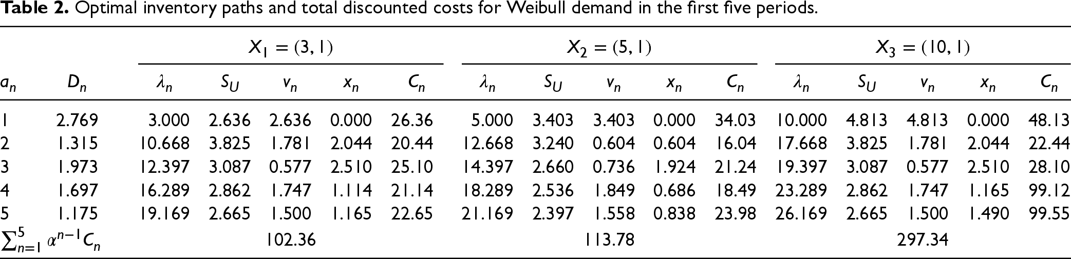
Using the standard inverse transform sampling method, we generate a sample path of random demands from the Weibull distribution with $m=2$ . Like Table 1, we tabulate the results for this in Table 2 for the three initial guesses: $X_1=(3,1)$ , $X_2=(5,1)$ , and $X_3=(10,1)$ .

Table 2.

Optimal inventory paths and total discounted costs for Weibull demand in the first five periods.

		$X_1=(3,1)$					$X_2=(5,1)$					$X_3=(10,1)$
$a_n$	$D_n$	${\lambda }_n$	$S_U$	$v_n$	$x_n$	$C_n$	${\lambda }_n$	$S_U$	$v_n$	$x_n$	$C_n$	${\lambda }_n$	$S_U$	$v_n$	$x_n$	$C_n$
1	2.769	3.000	2.636	2.636	0.000	26.36	5.000	3.403	3.403	0.000	34.03	10.000	4.813	4.813	0.000	48.13
2	1.315	10.668	3.825	1.781	2.044	20.44	12.668	3.240	0.604	0.604	16.04	17.668	3.825	1.781	2.044	22.44
3	1.973	12.397	3.087	0.577	2.510	25.10	14.397	2.660	0.736	1.924	21.24	19.397	3.087	0.577	2.510	28.10
4	1.697	16.289	2.862	1.747	1.114	21.14	18.289	2.536	1.849	0.686	18.49	23.289	2.862	1.747	1.165	99.12
5	1.175	19.169	2.665	1.500	1.165	22.65	21.169	2.397	1.558	0.838	23.98	26.169	2.665	1.500	1.490	99.55
$\sum _{n=1}^5{\alpha }^{n-1}{C}_n$		102.36					113.78					297.34

As before, we repeat the procedure for $N=1,000$ periods and compute $L_U(a_N)=0.034$ . For the three initial guesses ${\lambda }_1=3$ , 5, and 10, we obtain ${\lambda }_N={\lambda }_1+\sum _{i=1}^{N-1}{D}_i^2=4164.6$ , 4166.6, and 4180.2, respectively. The corresponding base-stock levels are $S_U({\lambda }_N,a_N)=0.034{\lambda }_N^{1/2}=2.189$ , 2.195, and 2.207, which are close to the asymptotic base-stock level of 2.190. The corresponding computation times (in seconds) for the three initial guesses are 5.73, 6.09, and 6.32, respectively.

7.3. Comparison With Myopic Policies in the Case of Exponential Demand

This subsection proposes two myopic policies in the exponential demand example of Subsection 7.2.1. Each uses the critical fractile formula for its updated demand distributions to obtain base-stock levels over time. We can then compute the cost achieved by each policy and compare it to the optimal cost.

First Myopic Policy: In period $n$ , we have the belief dependent upon the hyperparameters $X_n=(a_n,{\lambda }_n)$ . For the exponential demand, the updated CCDF on $X$ is (63), a gamma distribution with $m=1$ . Equating this to the critical fractile on the right-hand side of (72) gives us the base-stock level for that period. That is, we use

$$\overline{B}(S_n,X_n)={\left(\frac{{\lambda }_n}{{\lambda }_n+S_n}\right)}^{a_n}=\frac{c-\alpha c+\alpha h}{\alpha (h+p)},n=1,2,3,\dots ,$$

to obtain the base-stock levels

$$S_n={\lambda }_n(\frac{1}{{\left(\frac{c-\alpha c+\alpha h}{\alpha (h+p)}\right)}^{\frac{1}{a_n}}}-1),\text{where}n=1,2,3,\dots .$$

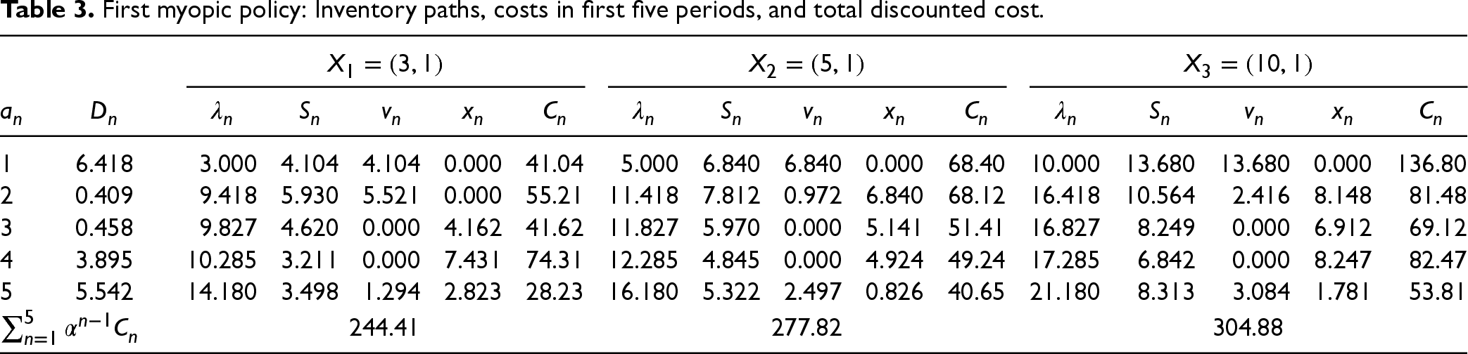
With these base-stock levels, we can summarize the first myopic policy results in Table 3, similar to Table 1 for the optimal base-stock levels.

Table 3.

First myopic policy: Inventory paths, costs in first five periods, and total discounted cost.

		$X_1=(3,1)$					$X_2=(5,1)$					$X_3=(10,1)$
$a_n$	$D_n$	${\lambda }_n$	$S_n$	$v_n$	$x_n$	$C_n$	${\lambda }_n$	$S_n$	$v_n$	$x_n$	$C_n$	${\lambda }_n$	$S_n$	$v_n$	$x_n$	$C_n$
1	6.418	3.000	4.104	4.104	0.000	41.04	5.000	6.840	6.840	0.000	68.40	10.000	13.680	13.680	0.000	136.80
2	0.409	9.418	5.930	5.521	0.000	55.21	11.418	7.812	0.972	6.840	68.12	16.418	10.564	2.416	8.148	81.48
3	0.458	9.827	4.620	0.000	4.162	41.62	11.827	5.970	0.000	5.141	51.41	16.827	8.249	0.000	6.912	69.12
4	3.895	10.285	3.211	0.000	7.431	74.31	12.285	4.845	0.000	4.924	49.24	17.285	6.842	0.000	8.247	82.47
5	5.542	14.180	3.498	1.294	2.823	28.23	16.180	5.322	2.497	0.826	40.65	21.180	8.313	3.084	1.781	53.81
$\sum _{n=1}^5{\alpha }^{n-1}{C}_n$		244.41					277.82					304.88

To obtain its total cost, we generate 1,000 sample paths of demands of $N$ = 200 periods based on the assumed true demand distribution. Since a cost of $1 in the 200th period is $\mathrm{\$}1\cdot {\alpha }^{200}\cdot \frac{1}{1-\alpha }=\mathrm{\$}1\cdot {0.9}^{200}\cdot 10\approx \mathrm{\$}7.05\times {10}^{-9}$ , a negligible number, we can ignore the total cost for the periods beyond 200. Thus, the total cost of the first 200 periods approximates the infinite horizon cost. Then, we average these costs associated with the 1,000 sample paths to obtain the expected total cost. Additionally, we calculate the average computational time (in seconds) and find values of 1.25, 1.30, and 1.28 for the three initial guesses of $X_1=(3,1)$ , $X_2=(5,1)$ , and $X_3=(10,1)$ , respectively. We report these results in Table 4.

Table 4.

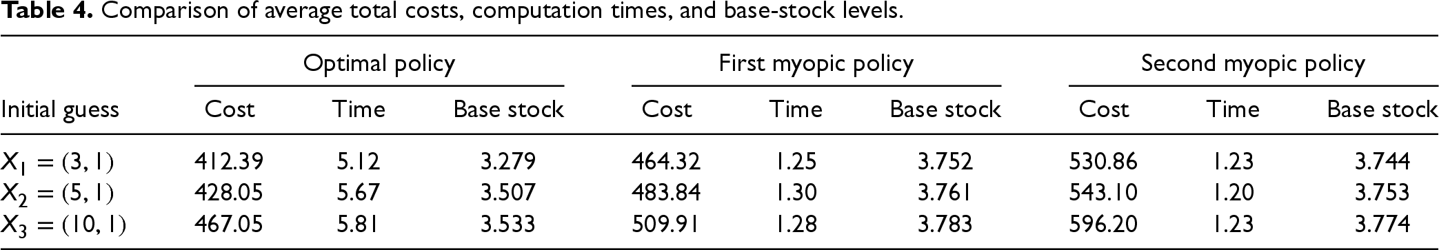
Comparison of average total costs, computation times, and base-stock levels.

	Optimal policy			First myopic policy			Second myopic policy
Initial guess	Cost	Time	Base stock	Cost	Time	Base stock	Cost	Time	Base stock
$X_1=(3,1)$	412.39	5.12	3.279	464.32	1.25	3.752	530.86	1.23	3.744
$X_2=(5,1)$	428.05	5.67	3.507	483.84	1.30	3.761	543.10	1.20	3.753
$X_3=(10,1)$	467.05	5.81	3.533	509.91	1.28	3.783	596.20	1.23	3.774

The updated demand distribution used in this policy is a gamma distribution, although the true demand distribution is exponential with the mean demand 4. As the introduction mentions, we can use a procedure that seeks updated distributions within the exponential class, and we can accomplish this by beginning with an initial belief about the mean demand and updating it each time we observe a new demand. Moreover, we already have the updated mean demand in period $n$ as ${\lambda }_n/a_n$ , a sufficient statistic for an exponential distribution. These observations justify the second suboptimal policy described below.

Second Myopic Policy: In period $n$ , the CCDF of the exponential distribution with the mean ${\lambda }_n/a_n$ is $e^{-\frac{a_n}{{\lambda }_n}{S}_n}=\frac{c-\alpha c+\alpha h}{\alpha (h+p)}.$ Then, the critical fractile formula gives optimal base-stock levels

$$S_n=-\frac{{\lambda }_n}{a_n}\ln \left(\frac{(1-\alpha )c+\alpha h}{\alpha (h+p)}\right),n=1,2,3,\dots .$$

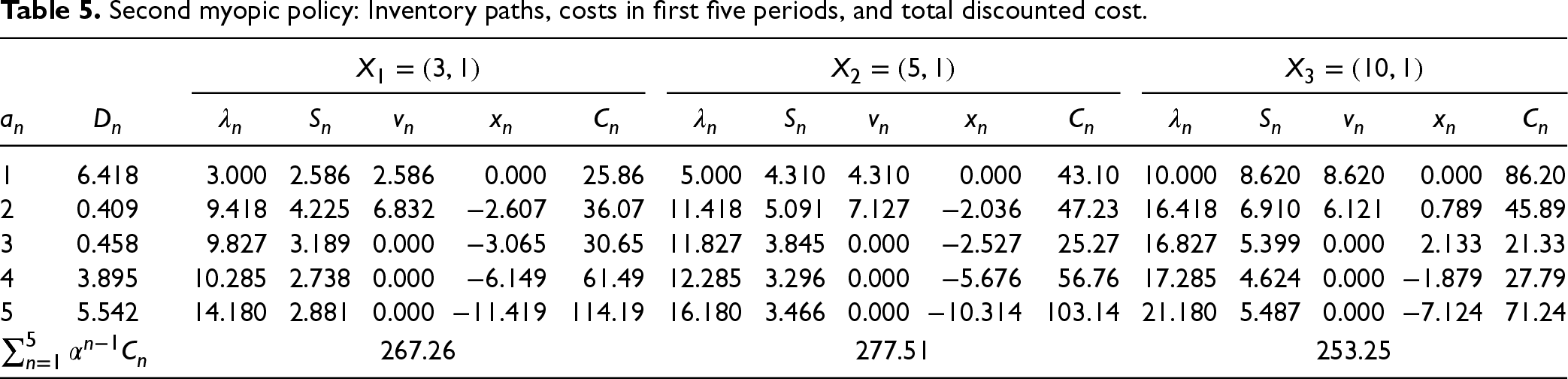
Treharne and Sox (2002) refer to such a policy as certainty equivalent control. Using these base-stock levels from the same 1,000 demand sample paths gives us the results in Table 5.

Table 5.

Second myopic policy: Inventory paths, costs in first five periods, and total discounted cost.

		$X_1=(3,1)$					$X_2=(5,1)$					$X_3=(10,1)$
$a_n$	$D_n$	${\lambda }_n$	$S_n$	$v_n$	$x_n$	$C_n$	${\lambda }_n$	$S_n$	$v_n$	$x_n$	$C_n$	${\lambda }_n$	$S_n$	$v_n$	$x_n$	$C_n$
1	6.418	3.000	2.586	2.586	0.000	25.86	5.000	4.310	4.310	0.000	43.10	10.000	8.620	8.620	0.000	86.20
2	0.409	9.418	4.225	6.832	$-2.607$	36.07	11.418	5.091	7.127	$-2.036$	47.23	16.418	6.910	6.121	0.789	45.89
3	0.458	9.827	3.189	0.000	$-3.065$	30.65	11.827	3.845	0.000	$-2.527$	25.27	16.827	5.399	0.000	2.133	21.33
4	3.895	10.285	2.738	0.000	$-6.149$	61.49	12.285	3.296	0.000	$-5.676$	56.76	17.285	4.624	0.000	$-1.879$	27.79
5	5.542	14.180	2.881	0.000	$-11.419$	114.19	16.180	3.466	0.000	$-10.314$	103.14	21.180	5.487	0.000	$-7.124$	71.24
$\sum _{n=1}^5{\alpha }^{n-1}{C}_n$		267.26					277.51					253.25

For the three initial guesses $X_1=(3,1)$ , $X_2=(5,1)$ , and $X_3=(10,1)$ , the total average discounted expected costs are 530.86, 543.10, and 596.20, and the average computational times (in seconds) are 1.23, 1.20, and 1.23. We report them in Table 4.

Using the same 1,000 demand sample paths, we can find the optimal base-stock levels utilizing the procedure in Subsection 7.2 for each sample path. We also report these results in Table 4.

Table 4 presents the average total costs, average computation times (in seconds) over 1,000 sample paths for a horizon of 200 periods, and base-stock levels in the 200th period for the three approaches: optimal, first myopic, and second myopic. The results show that the optimal policy achieves the lowest expected cost. Specifically, the percentage improvements by the optimal policy over the first myopic policy are 12.6%, 13.0%, and 9.2%, respectively, for the three initial guesses $X_1$ , $X_2$ , and $X_3$ . The corresponding improvements of the optimal policy over the second myopic policy are 28.7%%, 26.9%, and 27.7%. We also see that the first myopic policy dominates the second, consistent with the observation of Treharne and Sox (2002). These represent substantial losses of using myopic policies. On the other hand, as expected, the optimal policy requires more computational time, but not prohibitively more.

Finally, we want to point out that the base-stock levels in all three policies should converge to the true base-stock level of 3.448 in the limit. That is because, for the first myopic policy, we show in EC.7.3 in the E-Companion that the CCDF of the gamma distribution, reflecting the distribution of the updated demand given the hyperparameters, converges to the CCDF of the true Weibull distribution (which is the exponential distribution in our example). The result is evident in the second myopic policy case. As for the optimal policy, our computations indicate the march of the optimal base-stock levels over time. Moreover, in the march toward the true base-stock level of 3.448, the optimal policy does the best, and the first and second myopic policies follow it in that order.

8. When Demand Follows One of Two Distributions

We consider the case when the demand is known to come from one of two possible distributions, but we do not know which. For example, this could represent high-demand and low-demand environments. Thus, we model this in Subsection 8.1 by a belief function with a two-dimensional hyperparameter, which can be reduced to their ratio. We rewrite the functional equation for the particular case involving two exponential demands. This model of demand learning is new to the inventory literature with Bayesian updating, and it illustrates the generality of our approach. In Subsection 8.1.1, we develop a convenient approximation procedure involving iterations of the unique solution of the functional equation. In Subsection 8.1.2, we apply the method to an example of high and low exponential demands.

Let us consider the belief function $f(\xi )={\beta }_0\delta (\xi )+{\beta }_1\delta (\xi -1),$ where $\delta (\xi )$ and $\delta (\xi -1)$ represent the Dirac masses at 0 and 1, respectively, and ${\beta }_0$ and ${\beta }_1$ are hyperparameters. Since it is not a probability density, this writing is formal. We set the demands $g_0(z)=g(z|0)$ and $g_1(z)=g(z|1),$ which can be very general. We have

$$g(z|\xi )f(\xi )=g_0(z){\beta }_0\delta (\xi )+g_1(z){\beta }_1\delta (\xi -1),$$

(73)

which gives us a formal representation of the demand measure given the values ${\beta }_0$ and ${\beta }_1$ of the hyperparameters. It preserves, relating to $f(\xi ),$ the fact that it is also the sum of two Dirac measures at 0 and 1.

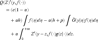
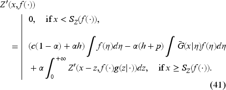
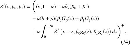
The functional $Z^{\mathrm{\prime }}(x,{\beta }_0\delta (\xi )+{\beta }_1\delta (\xi -1))$ in (42) can be written as $Z^{\mathrm{\prime }}(x,{\beta }_0,{\beta }_1),$ depending on the hyperparameters ${\beta }_0$ and ${\beta }_1$ instead of $f(.)$ , and it satisfies the equation

$$\begin{array}{rl}{Z}^{\mathrm{\prime }}(x,{\beta }_0,{\beta }_1)& =(\phantom{{\int }_0^{+\mathrm{\infty }}}(c(1-\alpha )+\alpha h)({\beta }_0+{\beta }_1)\\ & -\alpha (h+p)({\beta }_0{\overline{G}}_0(x)+{\beta }_1{\overline{G}}_1(x))\\ & {+\alpha {\int }_0^{+\mathrm{\infty }}{Z}^{\mathrm{\prime }}(x-z,{\beta }_0{g}_0(z),{\beta }_1{g}_1(z))dz)}^{+}.\end{array}$$

(74)

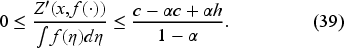
We can assume ${\beta }_0$ and ${\beta }_1$ to be strictly positive and set $\beta ={\beta }_0/{\beta }_1.$ Otherwise, if one is zero, we know the actual demand, and there is no need to learn. Since ${\beta }_0+{\beta }_1=1,$ we have

$${\beta }_0=\beta /(\beta +1)\text{and}{\beta }_1=1/(\beta +1).$$

(75)

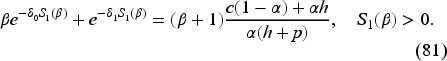
Noting (53), we have $Z^{\mathrm{\prime }}(x,{\beta }_0,{\beta }_1)=Z^{\mathrm{\prime }}(x,\beta {\beta }_1,{\beta }_1)=Z^{\mathrm{\prime }}(x,\beta ,1){\beta }_1.$ By setting $Z^{\mathrm{\prime }}(x,\beta )=Z^{\mathrm{\prime }}(x,\beta ,1)$ , we obtain immediately from (74) the following equation:

$$\begin{array}{rl}{Z}^{\mathrm{\prime }}(x,\beta )& =(\phantom{(x-z,\beta {\displaystyle \frac{g_0(z)}{g_1(z)}})}(c(1-\alpha )+\alpha h)(\beta +1)-\alpha (h+p)(\beta {\overline{G}}_0(x)\\ & {+{\overline{G}}_1(x))+\alpha {\int }_0^{+\mathrm{\infty }}{g}_1(z)Z^{\mathrm{\prime }}(x-z,\beta {\displaystyle \frac{g_0(z)}{g_1(z)}})dz)}^{+}.\end{array}$$

(76)

Thus, we are left only with one hyperparameter $\beta$ to learn from the demand observations. We solve (76) using an approximation method in the remainder of Section 8. We only consider the exponential demand case and develop an approximation in Subsection 8.1.1. In Subsection 8.1.2, we illustrate the method by a numerical example.

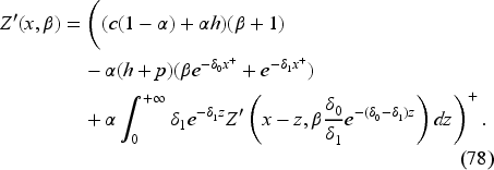
8.1. Exponential Demand Case

Let the demand densities be

$$g_0(z)={\delta }_0{e}^{-{\delta }_{0}z},g_1(z)={\delta }_1{e}^{-{\delta }_{1}z},$$

(77)

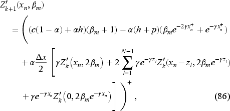
where ${\delta }_0>{\delta }_1$ . These densities represent low and high-demand environments, respectively, as their mean demands satisfy $1/{\delta }_0<1/{\delta }_1$ . The functional equation we need to solve is

$$\begin{array}{rl}{Z}^{\mathrm{\prime }}(x,\beta )& =(\phantom{(x-z,\beta {\displaystyle \frac{{\delta }_0}{{\delta }_1}}{e}^{-({\delta }_0-{\delta }_1)z})}(c(1-\alpha )+\alpha h)(\beta +1)\\ & -\alpha (h+p)(\beta e^{-{\delta }_0{x}^{+}}+e^{-{\delta }_1{x}^{+}})\\ & {+\alpha {\int }_0^{+\mathrm{\infty }}{\delta }_1{e}^{-{\delta }_{1}z}{Z}^{\mathrm{\prime }}(x-z,\beta {\displaystyle \frac{{\delta }_0}{{\delta }_1}}{e}^{-({\delta }_0-{\delta }_1)z})dz)}^{+}.\end{array}$$

(78)

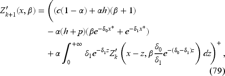
8.1.1. Iterative Approximation Procedure

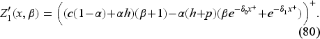
To compute the integral in equation (78), we iteratively refine our approximation of $Z^{\mathrm{\prime }}(x,\beta )$ . We accomplish this by rewriting (78), in the iterative form, as follows:

$$\begin{array}{rl}{Z}_{k+1}^{\mathrm{\prime }}(x,\beta )& =(\phantom{(x-z,\beta {\displaystyle \frac{{\delta }_0}{{\delta }_1}}{e}^{-({\delta }_0-{\delta }_1)z})}(c(1-\alpha )+\alpha h)(\beta +1)\\ & -\alpha (h+p)(\beta e^{-{\delta }_0{x}^{+}}+e^{-{\delta }_1{x}^{+}})\\ & {+\alpha {\int }_0^{+\mathrm{\infty }}{\delta }_1{e}^{-{\delta }_{1}z}{Z}_k^{\mathrm{\prime }}(x-z,\beta {\displaystyle \frac{{\delta }_0}{{\delta }_1}}{e}^{-({\delta }_0-{\delta }_1)z})dz)}^{+},\end{array}$$

(79)

starting with the initial guess

$$Z_1^{\mathrm{\prime }}(x,\beta )=((c(1-\alpha )+\alpha h)(\beta +1)-\alpha (h+p)(\beta e^{-{\delta }_0{x}^{+}}+e^{-{\delta }_1{x}^{+}}){)}^{+}.$$

(80)

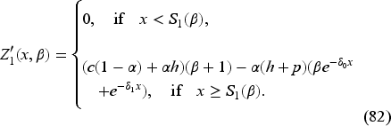
We first define $S_1(\beta )$ by solving

$$\beta e^{-{\delta }_0{S}_1(\beta )}+e^{-{\delta }_1{S}_1(\beta )}=(\beta +1){\displaystyle \frac{c(1-\alpha )+\alpha h}{\alpha (h+p)}},S_1(\beta )>0.$$

(81)

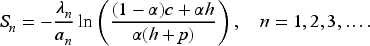
The function $S_1(\beta )$ is decreasing, and $Z_1^{\mathrm{\prime }}(x,\beta )$ is given by the following equation:

$$Z_1^{\mathrm{\prime }}(x,\beta )=\{\begin{array}{l}0,\text{if}x<S_1(\beta ),\\ \\ (c(1-\alpha )+\alpha h)(\beta +1)-\alpha (h+p)(\beta e^{-{\delta }_{0}x}\\ +e^{-{\delta }_{1}x}),\text{if}x\ge S_1(\beta ).\end{array}$$

(82)

Note that a straightforward but lengthy calculation shows (see EC.8.1 for details in the E-Companion) that $Z_2^{{}^{\prime }}(x,\beta )$ can be obtained as follows:

$$Z_2^{\mathrm{\prime }}(x,\beta )=\{\begin{array}{l}\begin{array}{rl}& 0,\text{if}x<S_2(\beta ),\\ \\ & (c(1-\alpha )+\alpha h)[\beta (1+\alpha (1-e^{-{\delta }_0{z}_1(x,\beta )}))\\ & +1+\alpha (1-e^{-{\delta }_1{z}_1(x,\beta )})]\\ & -\alpha (h+p)[e^{-{\delta }_{0}x}\beta (1+\alpha {\delta }_0{z}_1(x,\beta ))\\ & +e^{-{\delta }_{1}x}(1+\alpha {\delta }_1{z}_1(x,\beta ))],\text{if}x\ge S_2(\beta ),\end{array}\end{array}$$

(83)

where $z_1(x,\beta )$ is given in EC.8.1 in the E-Companion and $x=S_2(\beta )>0$ is the solution of

$$\begin{array}{rl}& (c(1-\alpha )+\alpha h)[\beta (1+\alpha (1-e^{-{\delta }_0{z}_1(x,\beta )}))\\ & +1+\alpha (1-e^{-{\delta }_1{z}_1(x,\beta )})]\\ & -\alpha (h+p)[e^{-{\delta }_{0}x}\beta (1+\alpha {\delta }_0{z}_1(x,\beta ))\\ & +e^{-{\delta }_{1}x}(1+\alpha {\delta }_1{z}_1(x,\beta ))]=0.\end{array}$$

(84)

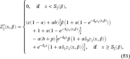
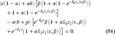
For $k\ge 2$ , we can only consider an approximate solution to (79). First, note that the upper limit for the integral in (79) can be replaced by $x$ because $Z_k^{\mathrm{\prime }}(x,\beta )=0$ for all $\beta$ when $x\le 0$ . Let

$$R=\{(x,\beta )|0\le x\le X,0\le \beta \le B\}$$

(85)

be a rectangle in the $x\beta$ -plane, and define a grid on $R$ with grid spacings $\mathrm{\Delta }x$ and $\mathrm{\Delta }\beta$ such that $N\mathrm{\Delta }x=X$ and $M\mathrm{\Delta }\beta =B$ . We compute $Z_{k+1}^{\mathrm{\prime }}(x,\beta )$ at the grid points $(x_n,{\beta }_m)=(n\mathrm{\Delta }x,m\mathrm{\Delta }\beta ),$ $0\le n\le N,$ $0\le m\le M,$ by approximating the integral in (79) using the composite trapezoidal formula

$$\begin{array}{rl}& Z_{k+1}^{\mathrm{\prime }}(x_n,{\beta }_m)\\ & =(\phantom{\sum _{l=1}^{N-1}}(c(1-\alpha )+\alpha h)({\beta }_m+1)-\alpha (h+p)({\beta }_m{e}^{-2\gamma x_n^{+}}+e^{-\gamma x_n^{+}})\\ & +\alpha {\displaystyle \frac{\mathrm{\Delta }x}{2}}[\phantom{\sum _{l=1}^{N-1}}\gamma Z_k^{\mathrm{\prime }}(x_n,2{\beta }_m)+2\sum _{l=1}^{N-1}\gamma e^{-\gamma z_l}{Z}_k^{\mathrm{\prime }}(x_n-z_l,2{\beta }_m{e}^{-\gamma z_l})\\ & {+\gamma e^{-\gamma x_n}{Z}_k^{\mathrm{\prime }}(0,2{\beta }_m{e}^{-\gamma x_n})\phantom{\sum _{l=1}^{N-1}}]\phantom{\sum _{l=1}^{N-1}})}^{+},\end{array}$$

(86)

where $z_l=l\mathrm{\Delta }x,$ $l=1,2,\dots ,N-1$ . This method extends the basic trapezoidal rule to handle integration over multiple subintervals, providing enhanced accuracy and efficiency. We use the trapezoidal rule within each subinterval to approximate the integral and sum the results to obtain the overall approximation. The method balances simplicity and accuracy, making it a popular choice for numerical integration. Our iterative approximation method uses the composite trapezoidal formula to efficiently approximate the integral defined in (78) over a predefined grid.

Since $Z_1^{\mathrm{\prime }}(x,\beta )$ is given explicitly by (80) during the computation of $Z_2^{\mathrm{\prime }}(x_n,{\beta }_m),$ $n=0,1,2,\dots ,N,$ $m=0,1,\dots ,M,$ the right-hand side of (86) is known precisely. For $k\ge 2$ , the second component of $(x_n-z_l,2{\beta }_m{e}^{-\gamma z_l})$ is not a grid value, and, therefore, we obtain $Z_k^{\mathrm{\prime }}(x_n-z_l,2{\beta }_m{e}^{-\gamma z_l})$ by interpolation using the neighboring grid point values.

For illustrative purposes, we set the parameter values as follows: $\alpha =0.9$ , $p=4$ , $c=10$ , and $h=1$ (as defined in Section 7), and let $N=40$ , $M=80$ , with $\mathrm{\Delta }x=0.1$ and $\mathrm{\Delta }\beta =0.05$ . In EC.8.2, we show the structure of the curves $Z_1^{\mathrm{\prime }}(x,\beta )$ , $Z_2^{\mathrm{\prime }}(x,\beta )$ , and $Z_3^{\mathrm{\prime }}(x,\beta )$ in ${\mathbb{R}}^3$ .

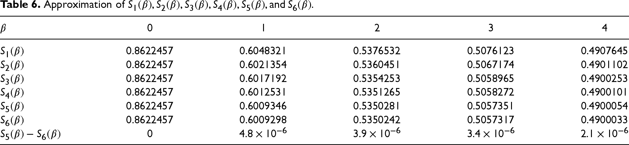
Knowing the data points $(x_n,{\beta }_m,Z_k^{\mathrm{\prime }}(x_n,{\beta }_m){)}_{\begin{array}{c}n=0,\dots ,N\\ m=0,\dots ,M\end{array}},$ we can extract the values

$$S_k({\beta }_m)=sup\{x_n|Z_k^{\mathrm{\prime }}(x_n,{\beta }_m)=0\}.$$

(87)

We use the convergence criterion of $\underset{k\ge 2}{sup}(S_{k-1}(\beta )-S_k(\beta ))<ϵ$ to terminate the iterative process. Specifically, we terminate the process once the change in successive iterations reaches the tolerance level $ϵ={10}^{-5}$ . Table 6 displays $S_k(\beta )$ for $k=1,2,3,4,5,6$ and $\beta =0,1,2,3,4$ . Based on these results, we use the approximation $S(\beta )\approx S_6(\beta )$ .

Table 6.

Approximation of $S_1(\beta ),S_2(\beta ),S_3(\beta ),S_4(\beta ),S_5(\beta ),\mathrm{and}{S}_6(\beta )$ .

$\beta$	0	1	2	3	4
$S_1(\beta )$	0.8622457	0.6048321	0.5376532	0.5076123	0.4907645
$S_2(\beta )$	0.8622457	0.6021354	0.5360451	0.5067174	0.4901102
$S_3(\beta )$	0.8622457	0.6017192	0.5354253	0.5058965	0.4900253
$S_4(\beta )$	0.8622457	0.6012531	0.5351265	0.5058272	0.4900101
$S_5(\beta )$	0.8622457	0.6009346	0.5350281	0.5057351	0.4900054
$S_6(\beta )$	0.8622457	0.6009298	0.5350242	0.5057317	0.4900033
$S_5(\beta )-S_6(\beta )$	0	$4.8\times {10}^{-6}$	$3.9\times {10}^{-6}$	$3.4\times {10}^{-6}$	$2.1\times {10}^{-6}$

8.1.2. Computation of Base-Stock Level for Exponential Demands

We consider the demand densities (77) with ${\delta }_0=2$ and ${\delta }_1=1$ , and the parameter values $\alpha =0.9$ , $p=4$ , $c=10$ , and $h=1$ as in Section 7. To demonstrate the implementation of our model, we assume that the true demand density is $g_0(z)=e^{-{\delta }_{0}z}$ . Then, the true mean is $1/{\delta }_0=1/2$ , and the asymptotic base-stock level computed using (72) is $S=0.4311$ . Since the IM does not know the true demand, he makes an initial guess of the hyperparameters ${\beta }_0>0$ and ${\beta }_1>0$ such that ${\beta }_0+{\beta }_1=1$ .

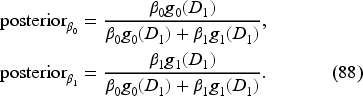
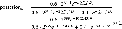
We use the predefined Matlab function exprnd(1/2, 1, 5) to generate $N=5$ simulated demands according to the true probability density $e^{-2z}$ . These are $D_1=0.1522$ , $D_2=0.9613$ , $D_3=0.1323$ , $D_4=0.0338$ , and $D_5=0.2135$ . Given (73), we obtain the posteriors of ${\beta }_0$ and ${\beta }_1$ as follows:

$$\begin{array}{rl}{\text{posterior}}_{{\beta }_0}& =\frac{{\beta }_0{g}_0(D_1)}{{\beta }_0{g}_0(D_1)+{\beta }_1{g}_1(D_1)},\\ {\text{posterior}}_{{\beta }_1}& =\frac{{\beta }_1{g}_1(D_1)}{{\beta }_0{g}_0(D_1)+{\beta }_1{g}_1(D_1)}.\end{array}$$

(88)

It is straightforward to see from (88) that ${\text{posterior}}_{{\beta }_0}+{\text{posterior}}_{{\beta }_1}=1$ in each period. We illustrate our model with two different guesses: $({\beta }_0,{\beta }_1)=(0.6,0.4)$ and $({\beta }_0,{\beta }_1)=(0.4,0.6)$ . These give us the initial $\beta =1.5$ and $\beta =2/3$ , respectively.

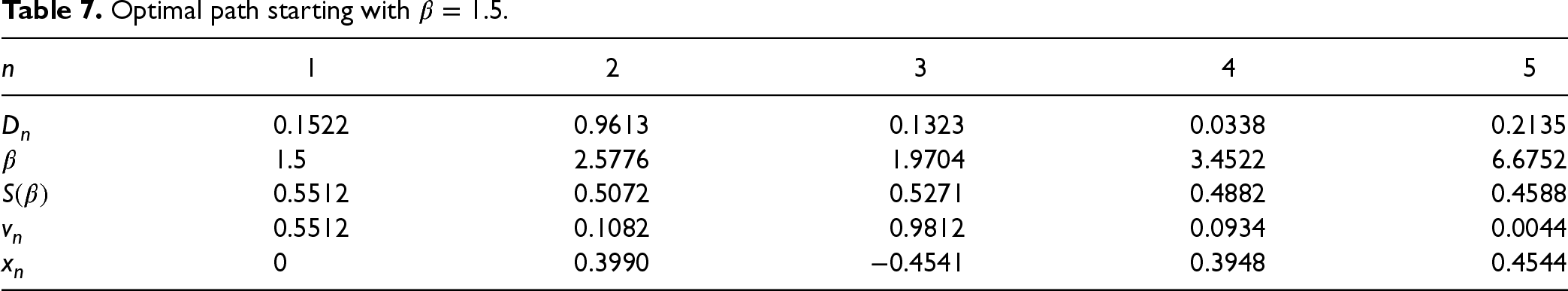
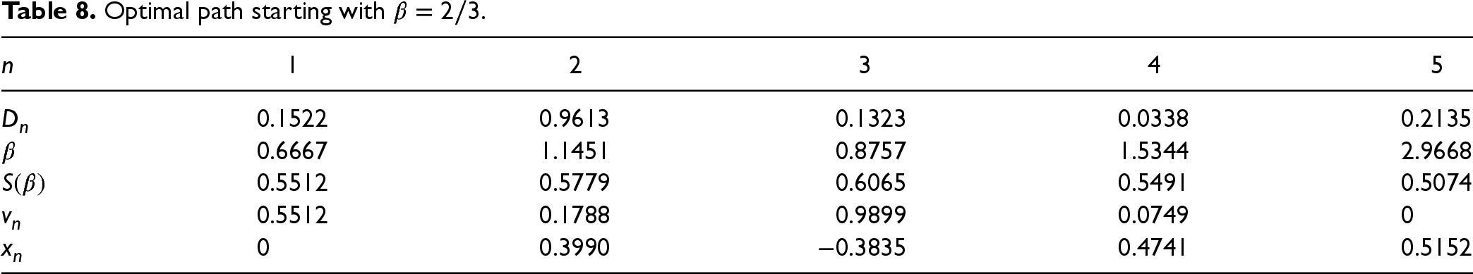
With $\beta =0.6/0.4=1.5$ , the base-stock level $S(1.5)=0.5512$ . Assuming the initial inventory $x_1=0$ , the order quantity $v_1=0.5512$ , giving $x_2=x_1+v_1-D_1=0.3990$ . In period 2, ${\beta }_0=0.6g_0(D_1)/0.6g_0(D_1)+0.4g_1(D_1)=0.7207$ , ${\beta }_1=0.4g_1(D_1)/0.6g_0(D_1)+0.4g_1(D_1)=0.2796$ , $\beta =0.6g_0(D_1)/0.4g_1(D_1)=2.5776$ , and the base-stock level $S(2.5776)=0.5072$ . Thus, the order quantity $v_2=0.1082$ and $x_3=-0.4541$ . This way, we can complete Table 7. Similarly, we complete Table 8 for the second initial guess $\beta =2/3.$

Table 7.

Optimal path starting with $\beta =\mathrm{1.5.}$

$n$	1	2	3	4	5
$D_n$	0.1522	0.9613	0.1323	0.0338	0.2135
$\beta$	1.5	2.5776	1.9704	3.4522	6.6752
$S(\beta )$	0.5512	0.5072	0.5271	0.4882	0.4588
$v_n$	0.5512	0.1082	0.9812	0.0934	0.0044
$x_n$	0	0.3990	$-0.4541$	0.3948	0.4544

Table 8.

Optimal path starting with $\beta =2/3.$

$n$	1	2	3	4	5
$D_n$	0.1522	0.9613	0.1323	0.0338	0.2135
$\beta$	0.6667	1.1451	0.8757	1.5344	2.9668
$S(\beta )$	0.5512	0.5779	0.6065	0.5491	0.5074
$v_n$	0.5512	0.1788	0.9899	0.0749	0
$x_n$	0	0.3990	‒ 0.3835	0.4741	0.5152

The fourth row in Tables 7 and 8 shows the base-stock level updates. As before, we generate $N=1,000$ demands according to the exponential density $g_0(z)$ and simulate for $N$ periods. We compute $S(1.5\cdot 2^{N-1}{e}^{-\sum _{i=1}^{N-1}{D}_i})=S(1.5\cdot 2^{999}{e}^{-501.2155})=0.4312$ and $S(2/3\cdot 2^{N-1}{e}^{-\sum _{i=1}^{N-1}{D}_i})=S(2/3\cdot 2^{999}{e}^{-501.2155})=0.4312$ . Both values are the same and close to the asymptotic base-stock level of 0.4311, with computation times (in seconds) of 4.41 and 4.13, respectively. We also observe that in period $N$ , our method has led to the value of the hyperparameter ${\beta }_0$ , which is very close to its true value of 1.

$$\begin{array}{rl}{\text{posterior}}_{{\beta }_0}& =\frac{0.6\cdot 2^{N-1}{e}^{-2\sum _{i=1}^{N-1}{D}_i}}{0.6\cdot 2^{N-1}{e}^{-2\sum _{i=1}^{N-1}{D}_i}+0.4\cdot e^{-\sum _{i=1}^{N-1}{D}_i}}\\ & =\frac{0.6\cdot 2^{999}{e}^{-1002.4310}}{0.6\cdot 2^{999}{e}^{-1002.4310}+0.4\cdot e^{-501.2155}}\approx 1.\end{array}$$

9. Concluding Remarks

We have considered a standard discrete-time infinite-horizon inventory problem with unknown general demand and backlog allowed. We begin with a general belief density prior and update it as the demand history unfolds. We prove the optimality of a belief-dependent base-sock policy by analyzing the resulting functional Bellman equation for the value function, which depends on the current inventory level and the current (updated) infinite-dimensional belief. We provide an iterative procedure to compute the optimal belief-dependent base-stock level for any given belief as the limit of a decreasing sequence of nonnegative numbers. We use the resulting stationary function offline to obtain the optimal base-stock levels over time as we update beliefs based on observed demands. We apply our methodology to the cases when the initial belief is a conjugate prior and when the true demand density belongs to one of two possible densities. Our method can be extended to handle the case of multiple possible densities, but we leave that for future research.

We illustrate our theory and the algorithm by solving a few numerical examples. In each example, the optimal base-stock levels march toward the asymptotic optimal value over time. Also, in the case of the example assuming exponential demand, we compare the performance of two critical-fractile-based myopic policies against the optimal policy and show that our policy results in significant cost reduction. For this example, we also prove that the optimal base-stock levels converge to a base-stock level, which is the optimal level in the corresponding infinite-horizon problem when the true demand distribution is known.

While the case of lost sales has been studied in the literature (reviewed in Section 2 and EC.1 1 in the E-Companion), our approach extends to this case, provided we can somehow infer the demands. Then, we can update the belief as in this article, and a base-stock policy would remain optimal. Finally, given that our method is quite general, exploring its applications to inventory problems with non-zero lead times and fixed ordering costs would be exciting topics for future research. In the lead-time case, we expect an optimal belief-dependent base-stock policy for the so-called inventory position. In the fixed-cost case, we expect a belief-dependent $(s,S)$ policy to be optimal.