Value-Partitioning of Sales Contribution in Business Markets

Abstract

In business markets, sales from customers are often jointly determined by multiple roles, yet firms struggle to quantify individual contribution of each role and the synergies among them. This study applies a value-partitioning approach to separate the sales contributions of customer-focused outside (OS) representatives (reps) and operations-focused inside (IS) reps, and their synergistic effects. It leverages variations in OS–IS combinations to generate individual-level value-added metrics, as well as metrics for dyadic synergies. To address empirical challenges such as limited variations in OS–IS combinations, the study employs empirical Bayes estimation, which provides best linear unbiased prediction (BLUP) estimates. An application using data from a Fortune 500 firm operating in business markets, reveals that the value added by OS reps, IS reps, and their interface have substantial and differential impacts on customer sales. Specifically, an increase of one standard deviation in the effect of OS, IS, or interface synergy improves customer sales by 17.8%, 11.6%, or 14.3%, respectively. Simulations demonstrate the superiority of empirical Bayes over fixed effects estimation in reducing bias, and that the value-added metrics are predictive of future customer sales. This research also illustrates how value-added metrics can be applied to evaluate the impact of sales programs on different sales roles.

1 Introduction

Sales processes in business markets involve multiple roles within selling firms, encompassing both customer-facing sales functions and internal operations and coordination processes. To add value for customers, sales organizations often rely on a combination of customer-focused representatives (known as outside sales (OS) reps) and operations-focused representatives (known as inside sales (IS) reps) (Highspot Team, 2023; Ryan, 2015). As boundary spanners, OS reps focus on interacting with customers to achieve sales quotas, whereas IS reps, in support roles for frontline employees, focus on managing operational aspects of sales activities. For example, when a customer seeks to upgrade a system, an OS rep engages with the customer, identifying needs and negotiating contracts, while the IS rep handles technical customer inquiries and coordinates with other operational functions (e.g., warehouse, logistics) to ensure timely order fulfillment. Although the titles and responsibilities may vary across firms, ¹ it is common in business markets for customers to be served by both relationship-building and operational process roles (e.g., Shi et al., 2024).

Effective management of dyadic selling requires firms to assess the individual contributions of OS and IS reps, along with their synergistic impact. Consider Firm ABC, which has implemented a sales automation platform designed primarily for IS reps, with features such as automated inventory reminders. To guide platform enhancements, the firm must evaluate how its existing features influence not only the sales contributions of IS reps but also their interactions with OS reps and the individual contributions of OS reps. For example, if the existing features significantly enhances IS reps’ value-added but inadvertently reduces interface value-added, the firm may need to investigate the changes in OS and IS reps’ interactions and possibly prioritize features to facilitate communications between OS and IS roles.

However, existing evaluation metrics are not well suited for this purpose. The common practice for evaluating sales contributions is to measure the total sales generated from the customers a rep has served (Johnston and Marshall, 2020; Mallapragada et al., 2022). However, team-based performance cannot differentiate the contributions from members and often leads to serious issues, including perceived unfairness, demotivation, and the risk of shirking or free riding (Kamei and Markussen, 2023). To separately evaluate individual behaviors, firms may use customer satisfaction surveys or self- or peer-evaluations; however, these ratings are prone to biases such as the inflation bias (Anderson et al., 1984), reciprocity bias (Magin, 2001), and halo effects (Balzer and Sulsky, 1992). ² Alternatively, firms can use activity-based metrics that focus on selling activities rather than outcomes, but such metrics encourage counterproductive behaviors such as prioritizing call quantity over quality or focusing on activity-based targets over meaningful sales targets (Forbes, 2014).

To overcome these challenges, we propose a value-partitioning approach that uses transaction data commonly accessible to selling firms in business markets via their customer relationship management (CRM) systems. The goal is to partition sales revenues into three sources of effects, i.e., value added by OS reps, IS reps, and their interfaces, as unobservable effects. By providing individual-level value-added metrics, this method enables alternative performance evaluation without relying on the measured characteristics of OS and IS reps.

The value-partitioning approach requires sufficient variations in OS and IS combinations. However, in practice, there usually is a moderate level of OS–IS variation, with most OS reps not collaborating with most IS reps; this situation creates a “small sample” challenge. To address this challenge, we propose to apply an empirical Bayes random-effect strategy to mitigate the estimation bias (Casella, 1985; Jackson, 2013). Compared to the baseline fixed effects (FE) estimation, it allows for correlations among the three effects and utilizes information from different groups (Koedel et al., 2015; Robinson, 1991), and produces best linear unbiased prediction (BLUP) ³ estimates for the metrics. Compared to traditional Bayesian random intercept estimation, empirical Bayes uses a fraction of computational resources and is considerably easier to implement, requiring less specialized knowledge.

To demonstrate the procedure of deriving value-added metrics, we analyze the data from a Fortune 500 company that operates in business markets. The dispersion of the distributions of the value-added metrics informs the role importance. We find that all three sources of value added have comparable and substantial impacts on customer sales. We find that value-added metrics can predict next year's customer sales better than simple metrics such as the total sales revenue across all customers one has served. Specifically, 79.2% (OS), 75.0% (IS), and 90.9% (synergy) effects of value-added estimates will be carried over to the next year.

We conduct simulations to assess the bias and accuracy of the proposed empirical Bayes estimation compared to the baseline FE estimation and simple joint sales revenue. We simulate synthetic datasets that accurately replicate the OS–IS combinations and the number of customers served by reps in the focal company. By varying unobserved customer effects, variety in OS–IS combinations, positive assortative pairing, and endogenous synergistic effects, we find that empirical Bayes outperforms both FE estimation and simple joint sales revenue.

Our proposed approach is tailored to the sales context involving two collaborative roles that jointly serve customers. It differs from prior research that examines role collaboration, such as OS and IS collaboration in Shi et al. (2024) and supervisor–employee fit in Hohenberg and Homburg (2019). These studies aim to enhance conceptual understanding by investigating how specific collaboration characteristics affect sales outcomes and empirically quantifying their impact (Gonzalez et al., 2014; Workman et al., 2003). In contrast, our study focuses on value-partitioning without relying on measured characteristics, aiming to provide an alternative performance evaluation metric. In addition, prior research may control for sales rep FE to obtain an unbiased estimation of measured collaboration characteristics, but they do not verify the suitability of FE as performance metrics (Shi et al., 2024).

With this research, we aim to make three primary contributions to academic literature and firm practice. First, we contribute to the marketing-operations interface research (Mallapragada et al., 2022; Vaid et al., 2021) by exploring the application of value-added metrics to partition the sales contributions of OS and IS sales roles. This approach enables firms to identify the sources of value—whether from individual reps or role interfaces—even when only joint outcomes are observable. The resulting metrics more accurately predict future customer sales than raw sales figures and support more effective targeting of churn interventions. Second, we develop a generalizable procedure, using empirical Bayes estimation, to derive value-added metrics from CRM data with the challenge of sparse OS–IS combinations. To help managers implement this approach, we provide a comprehensive guide that includes a step-by-step procedure, a use case, and accompanying Stata code and R scripts to illustrate the estimation process and how the metrics can be used to evaluate the impact of sales programs on different roles (see Web Appendix A). Third, we extend past research that examines the sales impact of observable characterstics in multiple role selling (Gonzalez et al., 2014; Hohenberg and Homburg, 2019; Shi et al., 2024; Workman et al., 2003). Unlike previous research, our value-partitioning approach offers a way to understand the sales impact of different roles that does not rely on the availability of observable characteristics.

2 Empirical Challenges

The lack of empirical evidence on the effects of OS, IS reps, and their interfaces stems mainly from the intertwined nature of their activities, which complicates effect separation.

2.1 Interdependence of OS and IS Reps in Business Markets

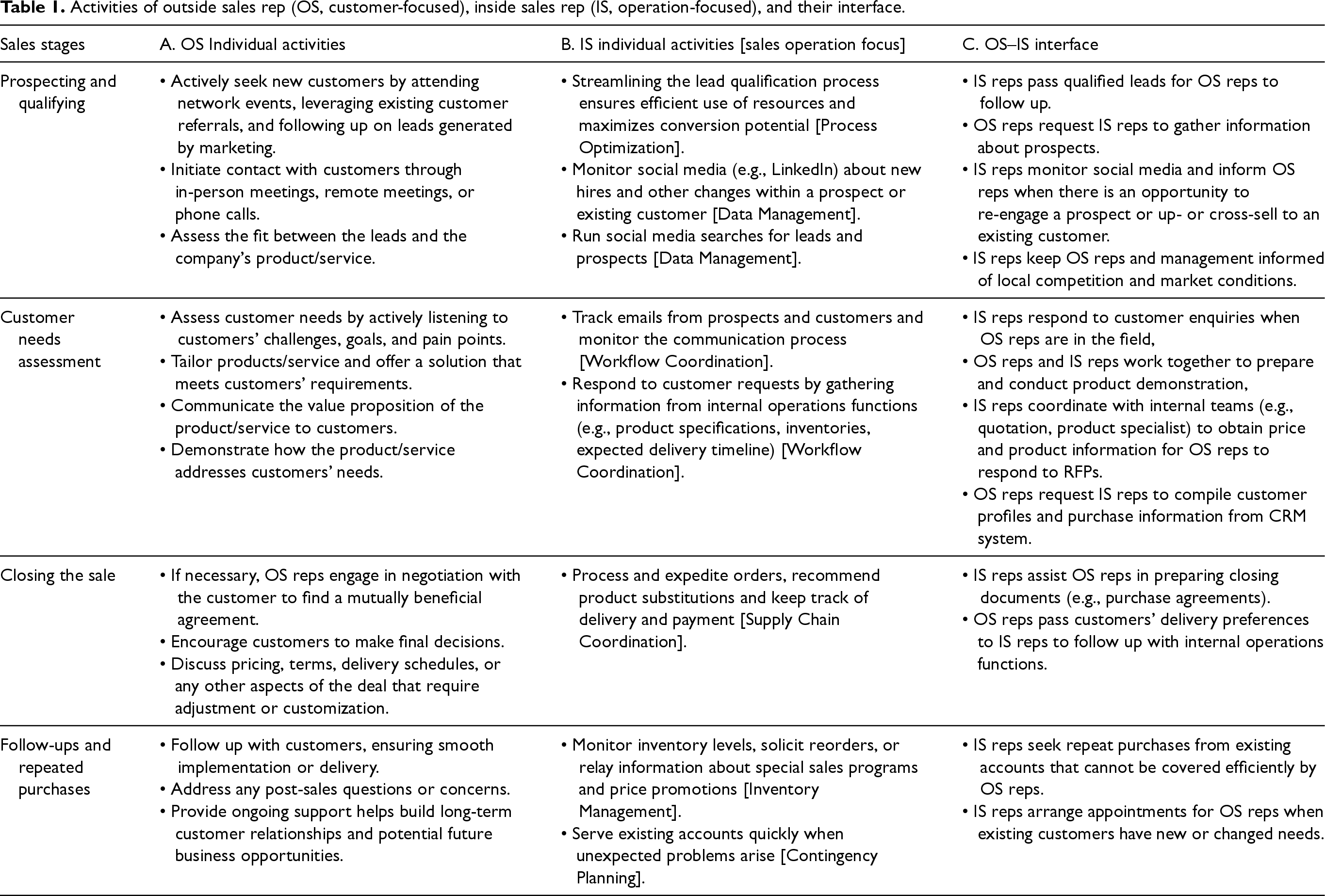
To understand the activities undertaken by OS and IS reps in business markets, we examined academic publications, practitioner articles, and job ads for OS and IS reps (see Web Appendix B). We categorized the activities of OS, IS reps, and their interfaces along four selling process stages (prospecting, presenting, closing, and following up; Table 1). The analysis reveals that OS reps focus on customer-focused activities (Column A). This includes tasks like actively seeking new customers, assessing customer needs, and building relationships. In contrast, IS reps engage in operation-focused activities (Column B). Their operations role in the sales process involves the administrative, analytical, and coordination activities that support front-line sales efforts by ensuring efficiency, accuracy, and seamless execution of sales-related tasks. This role involves back-office responsibilities that streamline workflows, manage data, facilitate customer interactions, and optimize sales execution. The categorization also highlights that OS and IS reps conduct activities jointly (Column C). These activities reflect the interface or synergy between the two roles and often involve tasks that require both customer-facing and operational expertise.

Table 1.

Activities of outside sales rep (OS, customer-focused), inside sales rep (IS, operation-focused), and their interface.

Sales stages	A. OS Individual activities	B. IS individual activities [sales operation focus]	C. OS–IS interface
Prospecting and qualifying	• Actively seek new customers by attending network events, leveraging existing customer referrals, and following up on leads generated by marketing. • Initiate contact with customers through in-person meetings, remote meetings, or phone calls. • Assess the fit between the leads and the company's product/service.	• Streamlining the lead qualification process ensures efficient use of resources and maximizes conversion potential [Process Optimization]. • Monitor social media (e.g., LinkedIn) about new hires and other changes within a prospect or existing customer [Data Management]. • Run social media searches for leads and prospects [Data Management].	• IS reps pass qualified leads for OS reps to follow up. • OS reps request IS reps to gather information about prospects. • IS reps monitor social media and inform OS reps when there is an opportunity to re-engage a prospect or up- or cross-sell to an existing customer. • IS reps keep OS reps and management informed of local competition and market conditions.
Customer needs assessment	• Assess customer needs by actively listening to customers’ challenges, goals, and pain points. • Tailor products/service and offer a solution that meets customers’ requirements. • Communicate the value proposition of the product/service to customers. • Demonstrate how the product/service addresses customers’ needs.	• Track emails from prospects and customers and monitor the communication process [Workflow Coordination]. • Respond to customer requests by gathering information from internal operations functions (e.g., product specifications, inventories, expected delivery timeline) [Workflow Coordination].	• IS reps respond to customer enquiries when OS reps are in the field, • OS reps and IS reps work together to prepare and conduct product demonstration, • IS reps coordinate with internal teams (e.g., quotation, product specialist) to obtain price and product information for OS reps to respond to RFPs. • OS reps request IS reps to compile customer profiles and purchase information from CRM system.
Closing the sale	• If necessary, OS reps engage in negotiation with the customer to find a mutually beneficial agreement. • Encourage customers to make final decisions. • Discuss pricing, terms, delivery schedules, or any other aspects of the deal that require adjustment or customization.	• Process and expedite orders, recommend product substitutions and keep track of delivery and payment [Supply Chain Coordination].	• IS reps assist OS reps in preparing closing documents (e.g., purchase agreements). • OS reps pass customers’ delivery preferences to IS reps to follow up with internal operations functions.
Follow-ups and repeated purchases	• Follow up with customers, ensuring smooth implementation or delivery. • Address any post-sales questions or concerns. • Provide ongoing support helps build long-term customer relationships and potential future business opportunities.	• Monitor inventory levels, solicit reorders, or relay information about special sales programs and price promotions [Inventory Management]. • Serve existing accounts quickly when unexpected problems arise [Contingency Planning].	• IS reps seek repeat purchases from existing accounts that cannot be covered efficiently by OS reps. • IS reps arrange appointments for OS reps when existing customers have new or changed needs.

The joint work of OS and IS reps within and across the sales stages makes it difficult to empirically separate the individual contributions of OS reps, IS reps, and the synergistic effects of their interface. This difficulty arises because the contributions of each role are not always easily attributable to individual actions but rather to a complex interplay of joint efforts.

2.2 Production of Customer Sales

Unlike the conventional view of the sales process (Figure 1, Panel A), where a single sales rep serves the customer (as in personal selling), Panel B illustrates the customer sales production process in OS–IS collaborative selling. OS–IS collaborative selling involves the effects of OS j's selling effort and IS k's selling effort, as well as the synergistic effect of OS j and IS k interface. To estimate these unobservable effects, we rely on customer-level sales data and customer–OS–IS links to decompose the variations in customer sales into effects that persist across customers served by (1) the OS, (2) the IS, and (3) the OS–IS dyad. Intuitively, we need sufficient variations in the matched relationships of customers, OS, and IS in the data. For example, if we consider only OS and IS individual effects, we need to observe that different sets of customers are served by OS rather than IS, to separate the OS individual effects from the IS individual effect. If an OS and an IS serve the same set of customers, the persistent effect across this set of customers represents the combined effects of the OS and the IS, and we cannot separate the two. The addition of the OS–IS interface effects further complicates the isolation of the sales rep effects. In the next section, therefore, we discuss the conditions required to identify the effects of OS, IS, and their interfaces separately.

Figure 1.

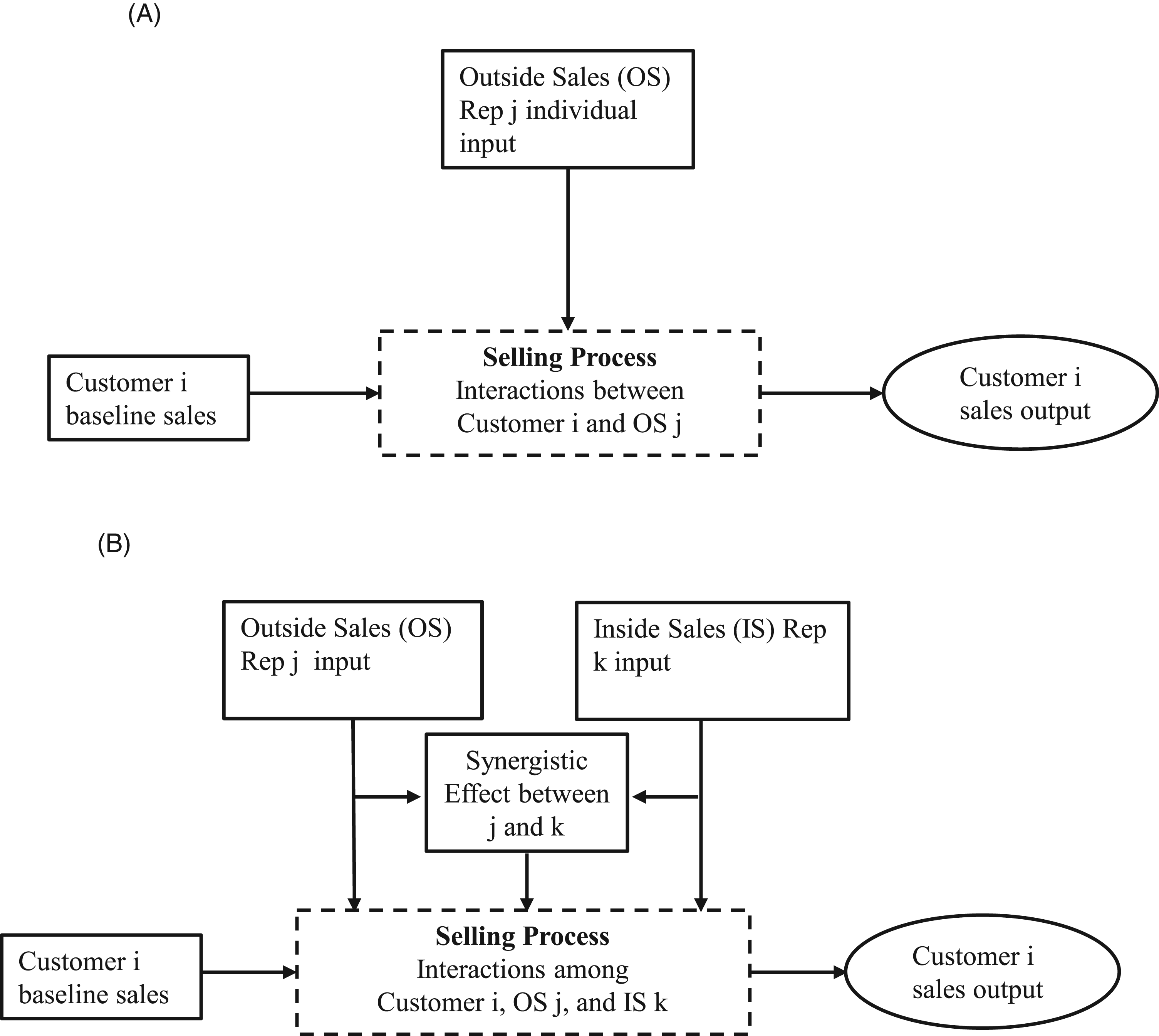
Sales reps’ role in production of customer sales. (A) Outside sales rep single-role selling; (B) Outside sales–inside sales reps collaborative selling.

3 Effect Separation

We consider the sales contributions of OS, IS, and their interfaces as unobservable effects. This approach does not rely on observable characteristics of OS and IS reps but requires customer-level sales outcomes and information about the links of customers, OS, and IS.

To describe the sales production process, we use a standard value-added model that is based on the Cobb–Douglas production function (Chan et al., 2014; Sridhar et al., 2011). Incorporation of the OS effect, the IS effect, and the OS–IS synergistic effect yields:

$$\begin{array}{r}\text{ln}(S_{ijk})={\theta }_j+{\theta }_k+{\theta }_{\text{jk}}+\gamma \text{ln}(S_{i_{base}})+\mathit{\delta }{\mathit{X}}_{\mathit{i}}+{\epsilon }_{ijk},\end{array}$$

(1)

where $S_{ijkt}$ is the sales outcome of customer i that is served by OS j and IS k, and ln(•) is the natural logarithmic function. The production technology includes three additively separable components: OS rep's individual effect ${\theta }_j$ , IS individual effect ${\theta }_k$ , and the synergy between the two reps ${\theta }_{jk}$ . ⁴ The Hicksian composite goods theorem (Hicks, 1939) and utility separability theory (Mas-Colell et al., 1995) justify modeling the three components as separable. The $S_{i\mathrm{\_}base}$ represents lagged customer sales, serving as baseline customer needs at the beginning of the evaluation period and considered a summary statistic for the full history of selling efforts input; ${\mathit{X}}_{\mathit{i}}$ is a vector of observable customer characteristics, and ${\epsilon }_{ijk}$ is an idiosyncratic error. The choice of covariates ( $S_{i\mathrm{\_}base}$ , ${\mathit{X}}_{\mathit{i}}$ ) depends on what the firm considers to be valuable sales contributions. ⁵

3.1 Ideal Empirical Setting

Separate quantification of ${\theta }_j$ , ${\theta }_k$ , and ${\theta }_{jk}$ requires variations in the combinations of OS and IS reps. A design with maximal variation would let any IS support all OS reps; a design with minimal variation would let each IS exclusively support one OS (Antony, 2014). We first discuss the effect separation in the ideal setting with maximal combination variation, then address other settings.

Using data on multiple IS reps supporting multiple OS reps, we can estimate IS–OS pair synergistic effects ( ${\theta }_{jk}$ ) separately from OS effects ( ${\theta }_j$ ) and IS effects ( ${\theta }_k$ ). As an illustration, consider two OS reps $j=\{1,2\}$ and two IS reps $k=\{\text{A},\text{B}\}$ ; each OS collaborates with both A and B, forming four OS–IS pairs. ⁶ Suppose each pair serves a nonempty set of customers $I_{jk}$ with the same observable characteristic variables. The set of customers served by each pair does not overlap. ⁷ We can isolate OS individual effects separately from IS individual effects, because the effects can be derived from the systematic variation of a different set of customers for each individual, that is, the persistent effect in the set of { $I_{1A}\cup I_{1B}$ } for OS 1, $\{I_{2A}\cup I_{2B}\}$ for OS 2, $\{I_{1A}\cup I_{2A}\}$ for IS A, and { $I_{1B}\cup I_{2B}\}$ for IS B, where $\cup$ represents the union of sets.

We also can isolate the OS–IS synergistic effects. To explain how, we denote the expected customer-sales-outcome difference between the pair of j and A and that of j and B as $E({\overline{S}}_{jA}-{\overline{S}}_{jB})$ . Note that we use S instead of $\text{ln}(S)$ to simplify the notation without compromising the reasoning. ${\overline{S}}_{jA}$ represents the mean of customer sales for the set of customers $I_{jA}$ , conditional on observed customer characteristics. $E({\overline{S}}_{jA}-{\overline{S}}_{jB})$ would be a consistent estimate for ( ${\theta }_A-{\theta }_B)+({\theta }_{j\text{A}}-{\theta }_{jB})$ , where ( ${\theta }_A-{\theta }_B)$ represents the individual effect difference between A and B, and $({\theta }_{j\text{A}}-{\theta }_{jB})$ represents the synergistic effect difference between the pair of j and A and the pair of j and B. Therefore,

$$\begin{array}{r}E({\overline{S}}_{jA}-{\overline{S}}_{jB})=({\theta }_A-{\theta }_B)+({\theta }_{j\text{A}}-{\theta }_{jB})\end{array}$$

(2)

If there are no synergistic effects, i.e., $({\theta }_{j\text{A}}-{\theta }_{jB})=0$ , then $E({\overline{S}}_{1A}-{\overline{S}}_{1B})=({\theta }_A-{\theta }_B),\text{and}E({\overline{S}}_{2A}-{\overline{S}}_{2B})=({\theta }_A-{\theta }_B)$ , based on equation (2) above. That is, with no synergistic effects, $E({\overline{S}}_{1A}-{\overline{S}}_{1B})-E({\overline{S}}_{2A}-{\overline{S}}_{2B})=0$ . However, with synergistic effects, $E({\overline{S}}_{1A}-{\overline{S}}_{1B})-E({\overline{S}}_{2A}-{\overline{S}}_{2B})=({\theta }_{1\text{A}}-{\theta }_{1B})-({\theta }_{2\text{A}}-{\theta }_{2B})\ne 0$ . Therefore, when multiple IS reps support multiple OS reps, we can separate the OS–IS synergistic effects from OS and IS individual effects.

3.2 OS–IS Combination Patterns Failing to Separate the Effects

In the previous discussion, we assumed that multiple OS support multiple IS. In other situations, we cannot separate all three effects ( ${\theta }_j,{\theta }_k,{\theta }_{jk}$ ). Consider three canonical situations.

3.2.1 One OS to one IS

In this setting, one OS works exclusively with one IS and vice versa, with a minimal combination of OS–IS. We cannot separately identify the three effects and can obtain only the estimates of the sum of the three effects. Consider two OS reps j = {1, 2} and two IS k = {A, B}, in which OS 1 collaborates only with IS A, and OS 2 collaborates only with IS B, forming two OS–IS pairs. Because the effects of OS1 and IS A are derived from the sales variation in the same set of customers $I_{1A}$ , and OS 2 and IS B from $I_{2B},$ we cannot separate the OS effects from IS effects. Following the same logic, the synergistic effects ${\theta }_{1A}$ and ${\theta }_{2B}$ rely on $I_{1A}$ and $I_{2B}$ , respectively, achieving collinearity with OS and IS individual effects. The difference in the outcomes—that is, $E({\overline{S}}_{1A}-{\overline{S}}_{2B})=({\theta }_1+{\theta }_A+{\theta }_{1A})-({\theta }_2+{\theta }_B+{\theta }_{2B})$ —identify only the aggregate effects or the sum of ${\theta }_j,{\theta }_k,\text{and}{\theta }_{jk}$ .

3.2.2 One OS to Multiple IS

In this setting, an OS collaborates with multiple IS reps, but one IS supports one OS. This setting allows us to separate the OS effect ${\theta }_j$ and the sum of ${\theta }_k\text{; and}{\theta }_{jk}$ . Consider two OS reps $j=\{1,\text{; }2\}$ and four IS reps $k=\{\text{A},\text{B},\text{C},\text{D}\}$ : OS 1 collaborates with IS A and B, and OS 2 collaborates with IS C and D. This setting cannot separate ${\theta }_k\text{and}{\theta }_{jk},$ because they are collinear and rely on the sales variation in the set of customers $I_{jk}$ (e.g., the estimation of ${\theta }_A$ and ${\theta }_{1A}$ rely on the same set $I_{1A}$ ). We can isolate OS effects because they rely on different sets of customers, that is, { $I_{1A}\cup I_{1B}$ } for OS 1 and $\{I_{2A}\cup I_{2B}\}$ for OS 2. ⁸ Therefore, this setting allows the separation of OS effects ${\theta }_j$ and the aggregate of ${\theta }_k\text{and}{\theta }_{jk}$ .

3.2.3 Multiple OS to one IS

In this setting, one OS collaborates only with one IS, and one IS supports two or more OS reps, mirroring the aforementioned “one OS to multiple IS” setting. Similarly, this setting allows the isolation of IS effects ${\theta }_k,$ the aggregate of OS effects ${\theta }_j$ and synergistic effects ${\theta }_{jk}.$ Web Appendix C summarizes the separation of the effects.

4 Empirical Context and Data

4.1 Empirical Context

To evaluate our approach, we use data from a leading U.S.-based distributor that sells industrial products and solutions that integrate lighting, sensors, switches, and relays, as well as hardware concerning data communications, networking, and electrical and power distribution systems. The company uses a field-based sales force, supported by IS reps, to sell products according to their geographical locations (see Shi et al. (2017, 2024) for studies using data from the same company). Similar to the general roles listed in Table 1, the OS reps of the company mainly acquire new customers and maintain customer relationships. The IS reps provide sales operational support functions throughout the stages of the selling process. A customer is served by a unique OS–IS dyad at any point in time, and dyad members share commissions based on jointly achieved sales. The commission rate for OS reps is 3–5 times higher than that of IS reps. The typical sales cycle lasts 3–6 months. Sales reps’ performance is evaluated quarterly to track short-term progress and annually for a comprehensive review.

The company's sales territory is organized into sales regions, and each sales region is divided into multiple sales branches. The company does not have formal guidelines for assigning customers to OS and IS reps. One OS–IS pair may serve multiple customers; one IS may support multiple OS; or one OS may receive support from multiple IS. After initiating contact with a customer, the OS follows through the selling process and maintains the relationship after the first purchase. An IS is usually assigned to a customer according to the IS's industry expertise and workload and continues to serve after the first purchase.

4.2 Data

The company possesses a CRM system that retains sales transactions dating to 2006 and incorporating information on OS and IS starting from 2008. A single transaction record contains identifiers of the customer, OS, IS, industry, region, invoice date, and sales amount. The company granted us access to its transactional records from 2008 to June 2014. Aligned with the company's performance evaluation cycle, we aggregated data to the unit of a customer-quarter and chose one year as the evaluation period for 2010–2013. We keep customers who are served by dyads with identifiable OS and IS and acquired in prior or earlier quarters as we focus on existing customers. We define value-added as the persistent effect of the rep on the actively transacting customers, measured on a per customer per quarter basis. In sample construction, we include actively transacting customers defined as those who had at least one transaction during that quarter. Web Appendix D summarizes the data by types of collaboration combinations for each year. We further keep the multiple OS–multiple IS setting, which accounts for more than 94% of total observations. The final sample had 112,940 customer-quarters.

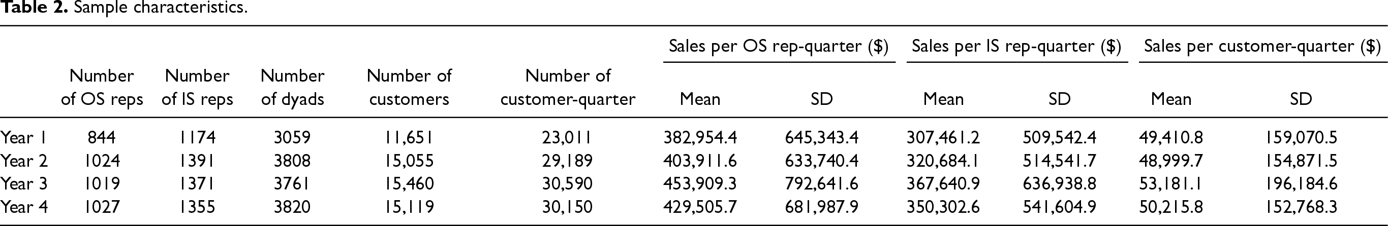
 Table 2 details the number of customers, OS reps, IS reps, and dyads year by year, along with the quarterly sales per customer, OS, and IS rep. The OS–IS combinations are sparse, with each rep typically working with an average of 3–4 reps in the other role. Each OS rep serves 7–8 active existing customers per quarter, and each IS rep serves 6–8. An average active customer contributes $49,411–$53,181 per quarter depending on the year. Table 3 provides the key descriptive statistics for the variables used in the analyses.

Table 2.

Sample characteristics.

						Sales per OS rep-quarter ($)		Sales per IS rep-quarter ($)		Sales per customer-quarter ($)
	Number of OS reps	Number of IS reps	Number of dyads	Number of customers	Number of customer-quarter	Mean	SD	Mean	SD	Mean	SD
Year 1	844	1174	3059	11,651	23,011	382,954.4	645,343.4	307,461.2	509,542.4	49,410.8	159,070.5
Year 2	1024	1391	3808	15,055	29,189	403,911.6	633,740.4	320,684.1	514,541.7	48,999.7	154,871.5
Year 3	1019	1371	3761	15,460	30,590	453,909.3	792,641.6	367,640.9	636,938.8	53,181.1	196,184.6
Year 4	1027	1355	3820	15,119	30,150	429,505.7	681,987.9	350,302.6	541,604.9	50,215.8	152,768.3

Table 3.

Descriptive statistics of key variables.

					Correlation
	Variable	Description	Mean	SD	1	2	3	4
1	Customer sales	Log-transformed customer quarterly sales	9.723	1.295	—
2	Lagged sales t−1	One quarter lagged customer sales (Log-transformed)	6.580	4.918	.416	—
3	Lagged sales t−2	Two quarter lagged customer sales (Log-transformed)	5.495	5.109	.309	.385	—
4	Customer Relationship tenure	Relationship tenure with the firm (months, log-transformed)	2.406	0.866	−.027	−.070	.233	—
5	National account	Dummy variable, equal to 1 if the customer is a national account, 0 otherwise	0.403	0.491	.089	.064	.119	.212

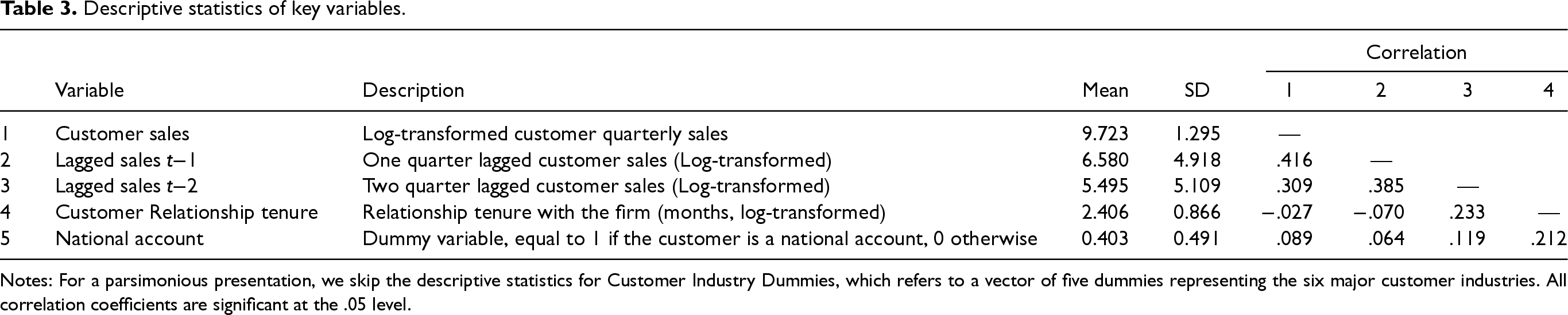
Notes: For a parsimonious presentation, we skip the descriptive statistics for Customer Industry Dummies, which refers to a vector of five dummies representing the six major customer industries. All correlation coefficients are significant at the .05 level.

5 Estimation

We first estimate value-added metrics using FE estimation as a baseline, then apply the proposed empirical Bayes random effects strategy that does not rely on large sample properties (Casella, 1985; Jackson, 2013).

5.1 Orthogonal FE Estimation

Researchers commonly use FE estimation to assess the contribution of one role (e.g., a teacher) to an outcome (Chetty et al., 2014; Koedel et al., 2015). The advantage of FE estimation is that it treats the effects for each rep as separate fixed parameters, without making assumptions about underlying distributions (Wooldridge, 2010). The estimates also are intuitive to interpret, capturing the constant impact of an individual rep on the customers served. To adapt the FE estimation to our context, we estimate:

$$\begin{array}{r}\text{ln}(S_{ijkq})={\theta }_j+{\theta }_k+\gamma \text{ln}(S_{i_{base}})+\mathit{\delta }{\mathit{X}}_{\mathit{i}}+{\epsilon }_{ijkq},\end{array}$$

(3)

with OS FE ${\theta }_j$ and IS FE ${\theta }_k$ . We define the synergistic effect for each OS–IS pair, ${\hat{\theta }}_{jk},$ as the mean of the residual ${\overline{\epsilon }}_{jk}$ for OS j and IS k across customers i and quarters q within an evaluation year (Jackson, 2013). That is, ${\overline{\epsilon }}_{jk}=\frac{1}{{\sum }_{q=1}^4{\sum }_{i=1}^{N_{jkq}}1}{\sum }_{q=1}^4{\sum }_{i=1}^{N_{jkq}}{\epsilon }_{ijkq}$ , where $N_{jkq}$ is the number of customers that OS j and IS k served in quarter q.

Because we calculate the synergistic effects from residuals, the estimated synergistic effects are orthogonal to OS and IS individual effects. The orthogonal synergistic effects have an intuitive interpretation: They represent observed within-OS variation in customer sales that can be attributed to collaborating with different IS reps. This approach relies on large-sample properties and can produce unbiased estimates if most OS reps collaborate with most IS reps. When there are limited variations in OS–IS combinations (i.e., an OS collaborates with only a few IS reps and vice versa), FE estimation mechanically loads synergistic effects, correlated with the OS effects or IS effects, onto the OS or IS effects (Jackson, 2013; Wooldridge, 2010). Therefore, it overstates the importance of OS and IS effects while understating the importance of synergistic effects. The need to account for small sample bias motivates us to use empirical Bayes random effect estimation.

5.2 Empirical Bayes Random Effect Estimation

Because of the limited variation in OS–IS combinations and the possibility of a small number of customers per dyad, along with the consideration of practicality for sales practitioners, we need an estimation method that (1) allows for potential correlation among individual effects of OS, IS, and their synergistic effects as opposed to the orthogonal FE estimation that forces the orthogonality between individual effects and synergistic effects; (2) leverages and borrows information across groups (i.e., customers grouped by OS, IS, and dyad) to produce stable and robust estimation, even for a small number of customers per group; (3) produces individual-level estimates (e.g., OS j's individual effect); and (4) is easy to implement for practical applications.

The empirical Bayes random effect estimation used by Jackson (2013) for estimating teacher and teacher–school match effects satisfies these requirements. It is a well-established technique within the Bayesian inference framework, used to address sparse data and small sample issues (Carter and Rolph, 1974; Casella, 1985; Efron and Morris, 1972). To implement, we first estimate equation (4) with OS–IS dyad FE:

$$\begin{array}{r}\text{ln}(S_{ijkq})=\gamma \text{ln}(S_{i\mathrm{\_}base})+\mathit{\delta }{\mathit{X}}_{\mathit{i}\mathit{q}}+{\pi }_{jk}+{\epsilon }_{ijkq},\end{array}$$

(4)

where ${\pi }_{jk}$ is the OS–IS dyad FE, and other notations are the same as equation (3). Because part of the dyad effect is attributed to these covariates, estimates of $\gamma$ and $\mathit{\delta }$ without dyad FE overstate the impact of ${\mathit{X}}_{\mathit{i}}$ and $\text{ln}(S_{i\mathrm{\_}base})$ (Chetty et al., 2014; Wooldridge, 2010). After obtaining the estimates $\hat{\gamma }$ and $\hat{\mathit{\delta }}$ , we compute the sales residual $R_{ijkq}$ :

$$\begin{array}{r}{R}_{ijkq}=\text{ln}(S_{ijkq})-(\hat{\gamma }\text{ln}(S_{i_{base}})+\hat{\mathit{\delta }}{\mathit{X}}_{\mathit{i}\mathit{q}}).\end{array}$$

(5)

We then use empirical Bayes estimation to estimate a random effect model:

$$\begin{array}{r}{R}_{ijkq}={\theta }_j^{EB}+{\theta }_k^{EB}+{\theta }_{jk}^{EB}+{\eta }_{ijkq},\end{array}$$

(6)

where ${\theta }_j^{EB}$ , ${\theta }_k^{EB}$ , and ${\theta }_{jk}^{EB}$ represents the empirical Bayes estimates of the value-added metrics.

The empirical Bayes estimation follows a two-step process (Casella, 1985). The first step involves using the entire data set to estimate the variances of the OS, IS, and synergistic effects by maximum likelihood estimation under the assumption of joint normality. This is the prior distribution for the model parameters. The second step combines this estimated prior and data associated with a group (e.g., customers served by OS j), using Bayes theorem to obtain the posterior estimates for that particular group (e.g., $\widehat{{\theta }_j^{EB}}$ ). The illustration of the detailed procedure is in the Web Appendix E.

The empirical Bayes estimation focuses on estimating the posterior mean of the parameters without producing full posterior distributions for each individual parameter, and the resulting posterior mean of each individual parameter is shrunk toward the population mean (i.e., mean of the estimated prior distribution in the first stage). The amount of shrinkage depends on the precision of the prior information (from the entire data), relative to the likelihood information from the group-specific data. If the prior information is strong, the estimates are more heavily influenced by the prior, resulting in more shrinkage toward the population mean. In addition, the predicted individual-level effects ( $\widehat{{\theta }_j^{EB}}$ , $\widehat{{\theta }_k^{EB}}$ , and $\widehat{{\theta }_{jk}^{EB}}$ ) from empirical Bayes estimation are the BLUPs that have minimum mean squared error (Jackson, 2013; Robinson, 1991). ⁹

Compared with FE estimation, the empirical Bayes random effect strategy has desirable features that make it a preferred estimation option for our data and research purpose. First, it addresses the issue with orthogonal FE estimation, which tends to overestimate individual effects and underestimate synergistic effects (Jackson, 2013; Wooldridge, 2010). By incorporating distributional information, the empirical Bayes estimator reduces these biases, providing more accurate estimates of both individual and synergistic effects. ¹⁰

Second, empirical Bayes random effect estimation is a “shrinkage” estimator that reduces the impact of extreme observations and helps stabilize the estimates, especially when there are limited data points for each group (individual or dyad in our context) (Snijders and Bosker, 2011). FE estimation does not have such a property and does not involve borrowing information from other groups (reps or dyads in our context) to obtain more stable estimates, which may produce unstable estimates when a small number of customers are observed by each rep or dyad.

6 Results

6.1 Evaluating the Overall Importance

We obtain value-added estimates for all three sources (i.e., OS individuals, IS individuals, and OS–IS interfaces) using both FE estimation and empirical Bayes estimation. Since sales are aggregated at the customer-quarter level and log-transformed, the unit of key independent variables (value-added metrics) is log-transformed sales, measured per customer per quarter. A larger effect signifies a higher value-added contribution to sales. For example, with OS rep effects, we can rank the OS reps based on their value-added estimates and generate summary statistics to describe their role importance. Although the means are set to zeros, the standard deviation (SD) of the OS individual effect is calculated to indicate the overall importance of the OS role, which can then be compared to the SDs of IS individual effect and OS–IS synergistic effect to understand their relative importance. For example, if the SD of OS and IS individual effects are ${\sigma }^{OS}$ and ${\sigma }^{IS}$ , respectively, a finding of ${\sigma }^{OS}$ $>{\sigma }^{IS}$ suggests that increasing the OS effect by 1 SD leads to a higher sales increase than increasing the IS effect by 1 SD (Chetty et al., 2014; Jackson, 2013). ¹¹

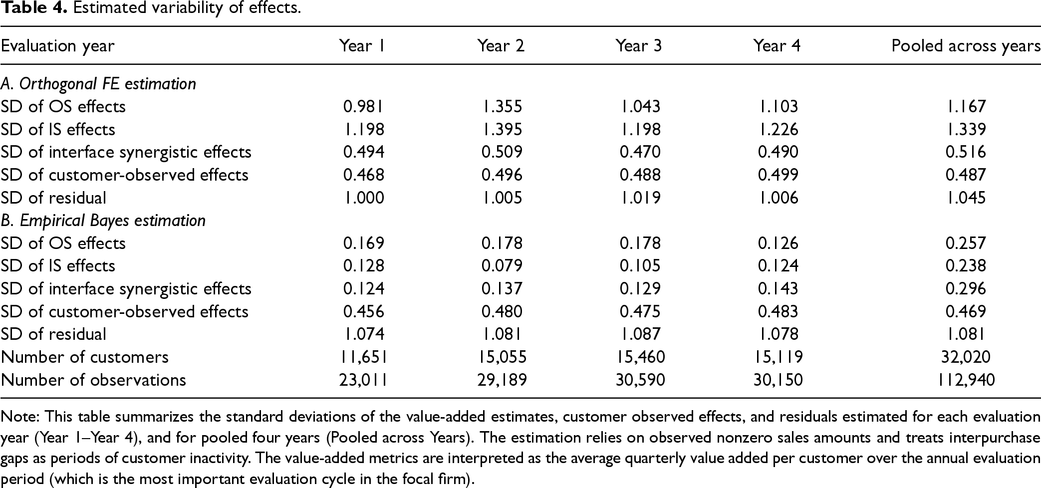
In Table 4, we present the SDs of the estimates with log-transformed quarterly customer sales for each evaluation year. As the estimates do not vary substantially across years, we focus on interpreting the estimates for the most recent year (Year 4). FE estimation (Table 4, Panel A) shows the SDs of the OS, IS, and synergistic effects are 1.103, 1.226, and .490, respectively, which implies that the importance of the OS role is slightly smaller than that of the IS role and is approximately double the importance of the synergistic effects. The SD values suggest that increasing each valued added effect by 1 SD from the average can generate 201.3% (OS), 240.8% (IS), and 63.2% (OS–IS interface) more sales per customer per quarter. ¹² In comparison, empirical Bayes finds the SDs of the OS, IS, and synergistic effects are 0.126, 0.124, and 0.143, respectively, which suggests comparable importance of three sources. The SD values suggest that increasing the effect by 1 SD from the average can generate 13.4% (OS), 13.2% (IS), and 15.4% (OS–IS interface) ¹³ more sales. A 1 SD increase in value-added corresponds to advancing approximately three or four deciles in rank for each role. FE estimation likely overestimates the sales contribution of each role due to the sparse OS–IS combinations, as we discussed in section 5.1, and we will rely on a simulation study to verify this, as will be discussed in section 6.3.

Table 4.

Estimated variability of effects.

Evaluation year	Year 1	Year 2	Year 3	Year 4	Pooled across years
A. Orthogonal FE estimation
SD of OS effects	0.981	1.355	1.043	1.103	1.167
SD of IS effects	1.198	1.395	1.198	1.226	1.339
SD of interface synergistic effects	0.494	0.509	0.470	0.490	0.516
SD of customer-observed effects	0.468	0.496	0.488	0.499	0.487
SD of residual	1.000	1.005	1.019	1.006	1.045
B. Empirical Bayes estimation
SD of OS effects	0.169	0.178	0.178	0.126	0.257
SD of IS effects	0.128	0.079	0.105	0.124	0.238
SD of interface synergistic effects	0.124	0.137	0.129	0.143	0.296
SD of customer-observed effects	0.456	0.480	0.475	0.483	0.469
SD of residual	1.074	1.081	1.087	1.078	1.081
Number of customers	11,651	15,055	15,460	15,119	32,020
Number of observations	23,011	29,189	30,590	30,150	112,940

Note: This table summarizes the standard deviations of the value-added estimates, customer observed effects, and residuals estimated for each evaluation year (Year 1–Year 4), and for pooled four years (Pooled across Years). The estimation relies on observed nonzero sales amounts and treats interpurchase gaps as periods of customer inactivity. The value-added metrics are interpreted as the average quarterly value added per customer over the annual evaluation period (which is the most important evaluation cycle in the focal firm).

6.2 Economic Interpretation of Estimated Effects

Translating the effect to dollars helps in understanding the impact of reassigning a customer to a more capable rep has on customer sales. To demonstrate this interpretation, we use the empirical Bayes estimates for Year 4 as an example. Consider a baseline scenario where a customer makes a $10,000 purchase in a quarter if served by average reps. Panel A of Figure 2 illustrates how the customer's purchase amount will change based on the value added by the assigned OS rep, ceteris paribus. If this customer is assigned to an OS rep whose value-added metric ranks in the bottom 10% among OS reps, the customer's purchase amount is expected to be $8316. If assigned to an OS rep in the top 10%, the customer's purchase amount averages $13,010. Panel B illustrates the relationship between the customer's purchase amount and the value added by the assigned IS rep. If assigned to an IS rep in the bottom 10% based on the value add metric, the customer's purchase amount averages $8219; if assigned to an IS rep in the top 10%, the customer's purchase amount averages $12,865. Panel C shows how the customer's purchase amount will change if the synergistic effect changes. If assigned to a dyad in the bottom 10% based on the synergistic effect rank, the customer's purchase amount averages $8048; if assigned to a dyad in the top 10%, the customer's purchase amount averages 13,473. Overall, the results suggest that all three sources have comparable effect sizes and substantial impacts on the firm's top-line performance (see the full distributions of the estimates in Web Appendix F).

Figure 2.

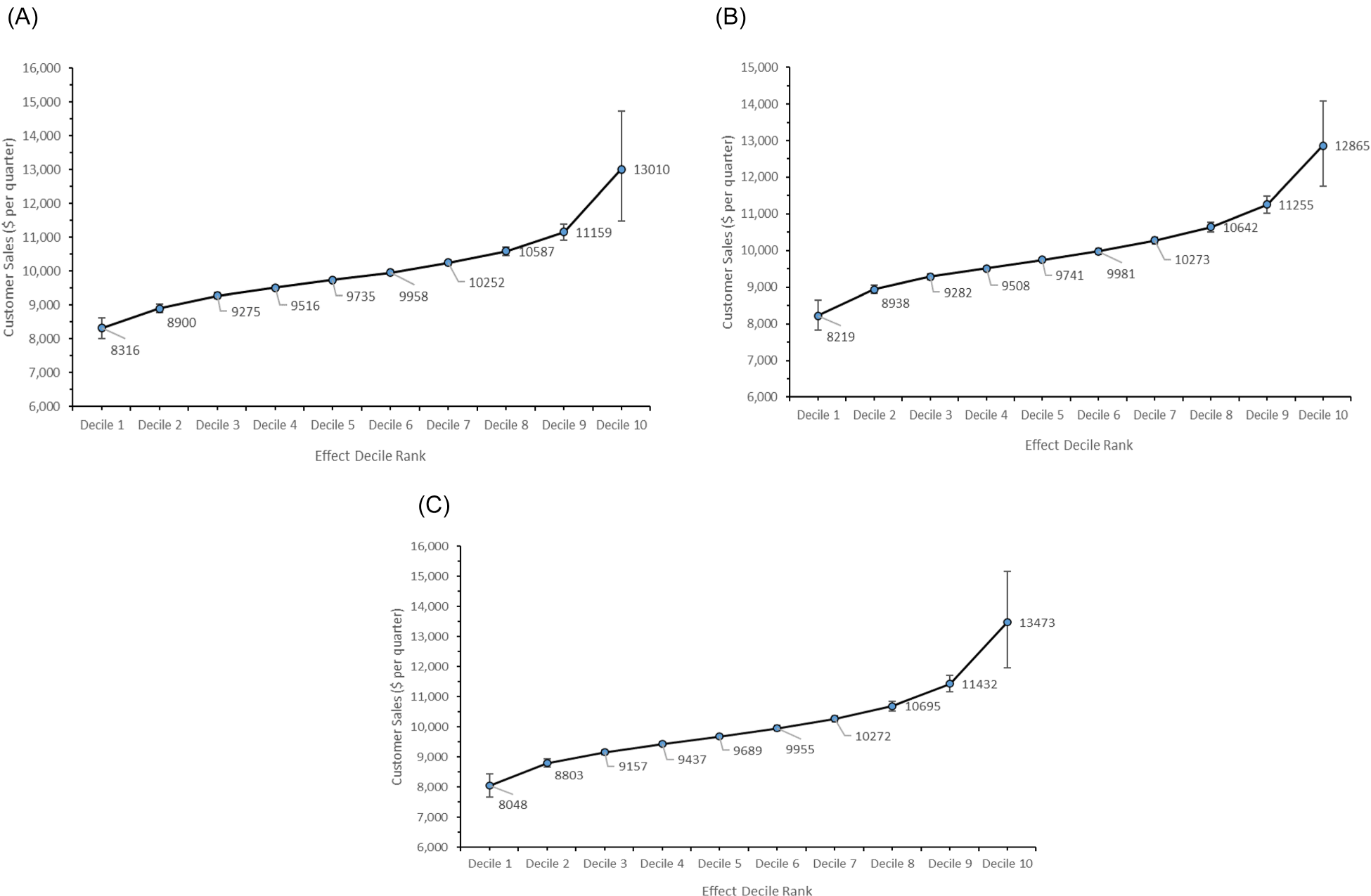
Economic interpretation of estimated effects. (A) Sales impact of outside sales individual; (B) Sales impact of inside sales individual; (C) Sales impact of synergistic effects. Notes: The graphs show the dollar amount of incremental sales driven by varying levels of individual rep value-added or OS–IS synergy. These estimates are calculated for a customer with a baseline of $10,000 in quarterly sales, assuming service by an average IS/OS rep with average synergistic effects. The x-axis represents different levels of value-added, grouped into deciles, with higher deciles indicating greater value-added. The y-axis represents the projected customer sales if served by reps or dyads at the corresponding deciles. Vertical bars around each mean indicate the standard deviation within that decile.

6.3 Comparing FE and Empirical Bayes Estimates

The differences between the two methods motivate us to assess which more accurately captures the true value-added. We begin by creating a synthetic data set that precisely replicates the OS–IS combinations and number of customers served by the reps and dyads in the focal company in Year 4. We assume that the log-transformed customer sales in quarter q, denoted as is an additive function of four elements: true value added by OS individual ( ${\theta }_j^{True}$ ), IS ( ${\theta }_k^{True}$ ), their synergistic effects ( ${\theta }_{jk}^{True}$ ), and unobserved customer-level effects ( $e_{ijkq}$ ). Specifically, $ln(S_{ijkq})={\theta }_j^{True}+{\theta }_k^{True}+{\theta }_{jk}^{True}+e_{ijkq}$ , where true value-added metrics and $e_{ijkq}$ are independently drawn from $Normal(0,0.5)$ . The resulting variation in sales is close to that of the focal company.

We next obtain empirical Bayes estimates ( ${\hat{\theta }}^{EB}$ ) and FE estimation ( ${\hat{\theta }}^{FE})$ . To measure bias, we regress ${\theta }^{True}$ on $\hat{\theta }$ and obtain $\lambda =\frac{cov({\theta }^{True},\hat{\theta })}{var(\hat{\theta })}$ , which is the coefficient of $\hat{\theta }$ from the regression (Chetty et al., 2014). $\lambda$ informs the relationship between $\hat{\theta }$ and ${\theta }^{True}$ , and $1-\lambda$ is the bias. We further use Root Mean Squared Error (RMSE) as an accuracy measure and Spearman rank correlation ¹⁴ as a rank preservation measure to describe the differences between $\hat{\theta }$ and ${\theta }^{True}$ .

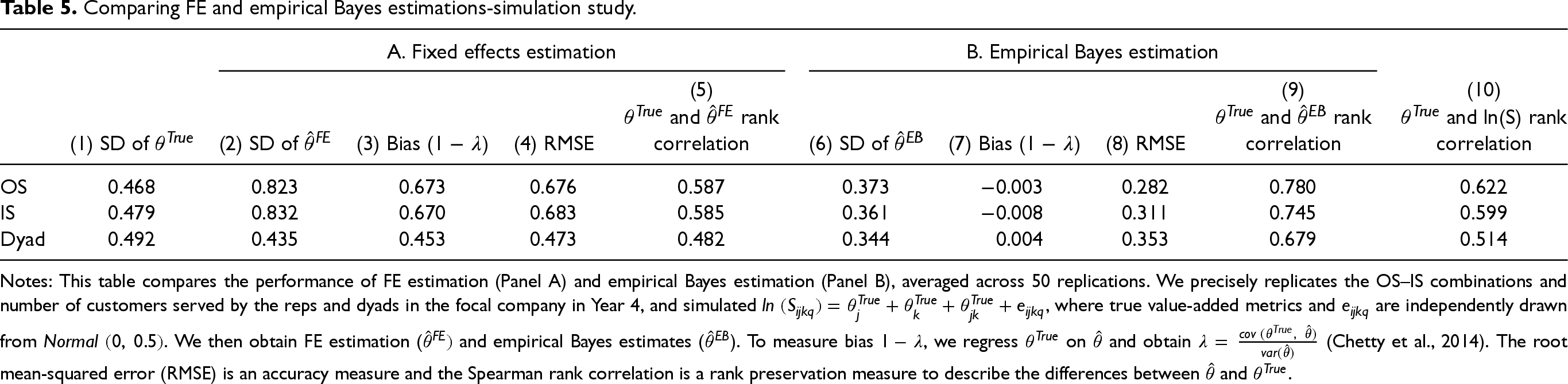
 Table 5 compares the performance of FE estimation (Panel A) and empirical Bayes estimation (Panel B), averaged across 50 replications. ¹⁵ It shows that the FE estimation produces SDs of ${\hat{\theta }}_j^{FE}$ , ${\hat{\theta }}_k^{FE}$ and ${\hat{\theta }}_{jk}^{FE}$ as 0.823, 0.832, and 0.435 respectively. The variations in the individual value-added are significantly inflated (Column 2), doubling the synergistic effects. Empirical Bayes yields SDs of ${\hat{\theta }}_j^{EB}$ , ${\hat{\theta }}_k^{EB}$ and ${\hat{\theta }}_{jk}^{EB}$ as 0.373, 0.361, and 0.344 (Column 6), moderately understating the true SDs but preserving the true relative magnitude well.

Table 5.

Comparing FE and empirical Bayes estimations-simulation study.

		A. Fixed effects estimation				B. Empirical Bayes estimation
					(5)				(9)	(10)
	(1) SD of ${\theta }^{True}$	(2) SD of ${\hat{\theta }}^{FE}$	(3) Bias (1 − $\lambda$ )	(4) RMSE	${\theta }^{True}$ and ${\hat{\theta }}^{FE}$ rank correlation	(6) SD of ${\hat{\theta }}^{EB}$	(7) Bias (1 − $\lambda$ )	(8) RMSE	${\theta }^{True}$ and ${\hat{\theta }}^{EB}$ rank correlation	${\theta }^{True}$ and ln(S) rank correlation
OS	0.468	0.823	0.673	0.676	0.587	0.373	−0.003	0.282	0.780	0.622
IS	0.479	0.832	0.670	0.683	0.585	0.361	−0.008	0.311	0.745	0.599
Dyad	0.492	0.435	0.453	0.473	0.482	0.344	0.004	0.353	0.679	0.514

Notes: This table compares the performance of FE estimation (Panel A) and empirical Bayes estimation (Panel B), averaged across 50 replications. We precisely replicates the OS–IS combinations and number of customers served by the reps and dyads in the focal company in Year 4, and simulated $ln(S_{ijkq})={\theta }_j^{True}+{\theta }_k^{True}+{\theta }_{jk}^{True}+e_{ijkq}$ , where true value-added metrics and $e_{ijkq}$ are independently drawn from $Normal(0,0.5)$ . We then obtain FE estimation ( ${\hat{\theta }}^{FE})$ and empirical Bayes estimates ( ${\hat{\theta }}^{EB}$ ). To measure bias $1-\lambda$ , we regress ${\theta }^{True}$ on $\hat{\theta }$ and obtain $\lambda =\frac{cov({\theta }^{True},\hat{\theta })}{var(\hat{\theta })}$ (Chetty et al., 2014). The root mean-squared error (RMSE) is an accuracy measure and the Spearman rank correlation is a rank preservation measure to describe the differences between $\hat{\theta }$ and ${\theta }^{True}$ .

In terms of estimation bias, empirical Bayes estimation significantly outperforms FE estimation. The biases of ${\hat{\theta }}_j^{EB}$ , ${\hat{\theta }}_k^{EB}$ , and ${\hat{\theta }}_{jk}^{EB}$ are −0.003, −0.008, and 0.004, respectively (Column 7). However, the biases of ${\hat{\theta }}_j^{FE}$ , ${\hat{\theta }}_k^{FE}$ , and ${\hat{\theta }}_{jk}^{FE}$ are significantly bigger, at 0.673, 0.670, and 0.453, respectively (Column 3). This finding suggests that empirical Bayes estimation produces estimates with minimal biases, whereas FE estimation produces large biases.

Regarding accuracy, empirical Bayes estimation also outperforms the FE estimation. The RMSEs produced by empirical Bayes range from 0.282–0.353; in contrast, those produced by FE estimation range from 0.473–0.683 (see Columns 8 and 4). The rank correlation between ${\theta }^{True}$ and empirical Bayes $\hat{\theta }$ are 0.780 (OS), 0.745 (IS), and 0.679 (synergistic effect). These correlations are higher compared to those between ${\theta }^{True}$ and FE $\hat{\theta }$ , which are at 0.587, 0.585, and 0.482 (see Columns 9 and 5). Therefore, in addition to smaller biases, empirical Bayes estimation demonstrates superior accuracy compared to FE estimation.

To benchmark against the practice of using joint sales revenue for performance evaluation, we also calculated the rank correlation between ${\theta }^{True}$ and $ln(S_{ijkq})$ (Column 10). The correlations range from 0.514 to 0.622, lower than those with empirical Bayes but slightly higher than those with FE estimates.

As the distributions of the value-added estimates show long right tails (Web Appendix F), we conduct a set of simulations where the true value-added metrics are deliberately made non-Gaussian and right skewed. Our results (Web Appendix G) show that empirical Bayes estimates remain robust under these conditions: the biases are minimal, and the rank-based metrics continue to outperform both FE estimations and raw sales. Therefore, empirical Bayes estimation is superior to FE estimation and more accurate than using joint sales revenue for the focal firm.

6.4 Leveraging OS, IS Reassignments

Nonrandom OS–IS sorting can introduce bias in empirical Bayes estimation. We assess this bias by considering within-customer value-added changes such as the rep re-assignments that we observe in our data. Customers may experience changes in the reps supporting them over time due to various reasons such as turnover, rotation, extended leave, etc. If a customer's OS changes but IS does not, we expect that customer sales should change by the individual effect difference between the two OS reps and the synergistic effect difference between the two dyads. The identifying assumption for this evaluation is that the unobserved variables influencing a previous OS–IS pairing differ from those affecting a subsequent OS–IS pairing. This is highly plausible in our context because pairings are influenced by varying unobserved variables which are situational factors, including workload, lead assignment, and sales managers in charge.

The within-customer rep changes, however, do not allow us to separate individual effects and synergistic effects, because whenever there is a change in rep, it always results in a change in dyad. For example, when a customer's OS rep changes from j to j* while the IS rep k remains the same, the value added for this customer changes from ${\theta }_j+{\theta }_{jk}$ to ${\theta }_{j*}+{\theta }_{j*k}$ . This allows us to assess the bias in the aggregate effect of an OS or IS rep and its synergistic effects.

To assess the bias of the aggregate of OS reps and their synergistic effects, we obtain the sales residual ( ${\text{RES}}_{ijkq}^{OS\mathrm{\_}syn}$ ) by subtracting the value added by IS k in year y ( ${\hat{\theta }}_{ky}^{EB}$ ) from $R_{ijkq}$ in equation (5):

$$\begin{array}{r}{\text{RES}}_{ijkq}^{OS\mathrm{\_}syn}=R_{ijkq}-({\hat{\theta }}_{ky}^{EB})\end{array}$$

(7)

As we pool data across four years, we use “y” in the subscript to represent the year. ${\hat{\theta }}_{jy}^{EB}$ represents the value added by OS j in year y. ${\hat{\theta }}_{jky}^{EB}$ represents the empirical Bayes estimated value added by the synergy of OS j and IS k in year y. We then regress ${\text{RES}}_{ijkq}^{OS\mathrm{\_}syn}$ on ${\hat{\theta }}_{jy}^{EB}+{\hat{\theta }}_{jky}^{EB}$ with customer FE:

$$\begin{array}{r}{\text{RES}}_{ijkq}^{OS\mathrm{\_}syn}={\lambda }_{OS\mathrm{\_}syn}({\hat{\theta }}_{jy}^{EB}+{\hat{\theta }}_{jky}^{EB}\text{; })+{\alpha }_i+{\zeta }_{ijkq}.\end{array}$$

(8)

By adding the customer FE ${\alpha }_i$ , we rely on within-customer variation to estimate ${\lambda }_{OS\mathrm{\_}syn}$ , and $1-{\lambda }_{OS\mathrm{\_}syn}$ represents the bias. We use the same way to obtain $1-{\lambda }_{IS\mathrm{\_}syn}$ :

$$\begin{array}{rl}{\text{RES}}_{ijkq}^{IS\mathrm{\_}syn}& =R_{ijkq}-({\hat{\theta }}_{jy}^{EB})\end{array}$$

(9)

$$\begin{array}{rl}{\text{RES}}_{ijkq}^{IS\mathrm{\_}syn}& ={\lambda }_{IS\mathrm{\_}syn}({\hat{\theta }}_{ky}^{EB}+{\hat{\theta }}_{jky}^{EB})+{\alpha }_i+{\zeta }_{ijkq}\end{array}$$

(10)

Among the 32,020 unique customers in the four years of data, 4205 experienced OS changes; 6030 experienced IS changes. For the evaluation, we retain customers who experience at least one incidence of rep change (OS or IS) and retain dyads that at least serve five customers in a year. The resulting sample involves 43,391 customer-quarters with 7714 customers, 1158 OS reps, and 1352 IS reps.

 Table 6 reports the analysis results. The estimate of ${\lambda }_{OS\mathrm{\_}syn}$ is 1.041, indicating a bias of −0.041. The estimate of ${\lambda }_{IS\mathrm{\_}syn}$ is 1.066 (a bias of −0.066). If our identifying assumption is correct, our within-customer investigation suggests that the between-customer value-added estimates show minimal nonrandom sorting bias.

Table 6.

Bias evaluation using within-customer rep changes.

	Coefficient estimate ( ${\lambda }_{OS\mathrm{\_}syn}$ )	Standard error	Bias ( $1-{\lambda }_{OS\mathrm{\_}syn})$
${\hat{\theta }}_{jy}^{EB}+{\hat{\theta }}_{jky}^{EB}$	1.041	0.030	−0.041
Intercept	−0.026	0.004
R-square	0.449
	Coefficient Estimate ( ${\lambda }_{\text{IS}\mathrm{\_}syn}$ )	Standard Error	Bias ( $1-{\lambda }_{\text{IS}\mathrm{\_}syn}$ )
${\hat{\theta }}_{ky}^{EB}+{\hat{\theta }}_{jky}^{EB}$	1.066	0.031	−0.066
Intercept	−0.025	0.004
R-square	0.437

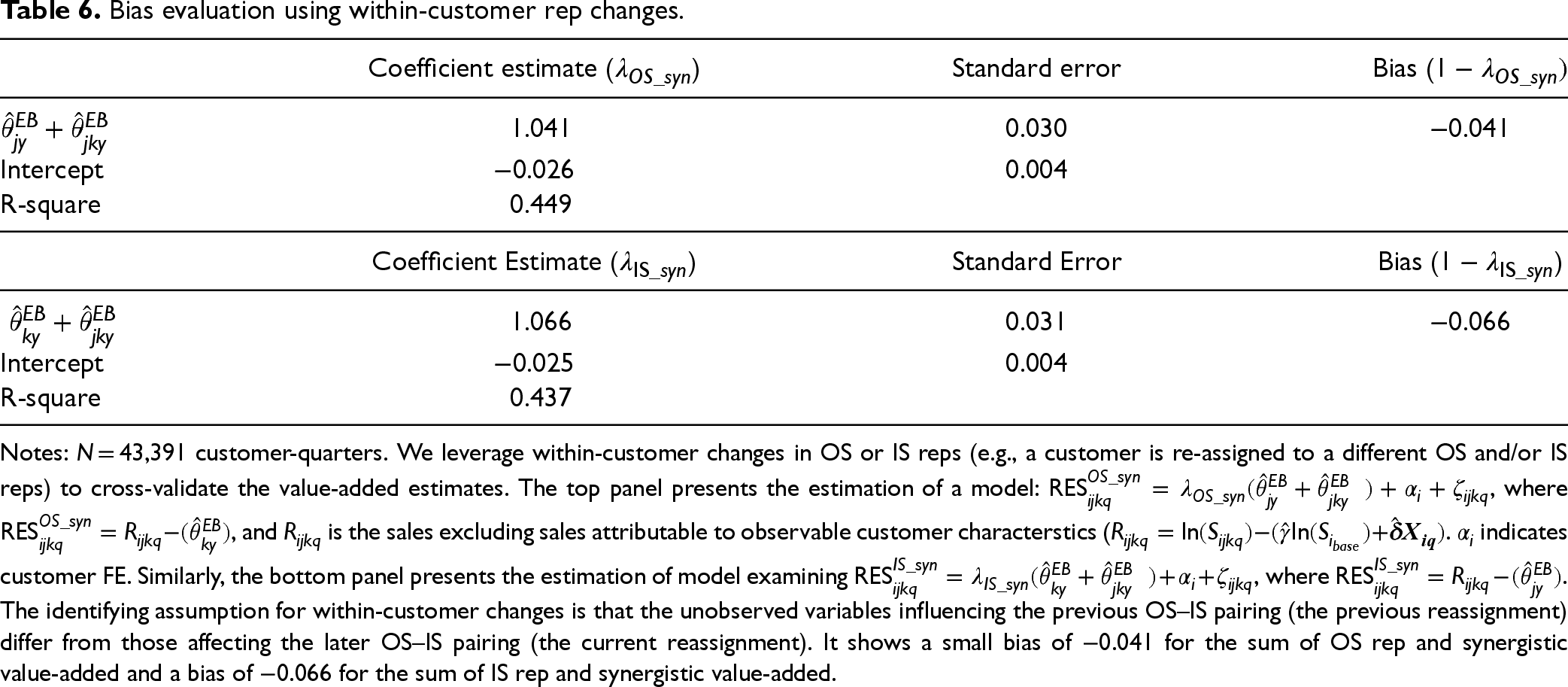
Notes: N = 43,391 customer-quarters. We leverage within-customer changes in OS or IS reps (e.g., a customer is re-assigned to a different OS and/or IS reps) to cross-validate the value-added estimates. The top panel presents the estimation of a model: ${\text{RES}}_{ijkq}^{OS\mathrm{\_}syn}={\lambda }_{OS\mathrm{\_}syn}({\hat{\theta }}_{jy}^{EB}+{\hat{\theta }}_{jky}^{EB}\text{; })+{\alpha }_i+{\zeta }_{ijkq}$ , where ${\text{RES}}_{ijkq}^{OS\mathrm{\_}syn}=R_{ijkq}-({\hat{\theta }}_{ky}^{EB})$ , and $R_{ijkq}$ is the sales excluding sales attributable to observable customer characterstics ( $R_{ijkq}=\text{ln}(S_{ijkq})-(\hat{\gamma }\text{ln}(S_{i_{base}})+\hat{\mathit{\delta }}{\mathit{X}}_{\mathit{i}\mathit{q}})$ . ${\alpha }_i$ indicates customer FE. Similarly, the bottom panel presents the estimation of model examining ${\text{RES}}_{ijkq}^{IS\mathrm{\_}syn}={\lambda }_{IS\mathrm{\_}syn}({\hat{\theta }}_{ky}^{EB}+{\hat{\theta }}_{jky}^{EB}\text{; })+{\alpha }_i+{\zeta }_{ijkq}$ , where ${\text{RES}}_{ijkq}^{IS\mathrm{\_}syn}=R_{ijkq}-({\hat{\theta }}_{jy}^{EB})$ . The identifying assumption for within-customer changes is that the unobserved variables influencing the previous OS–IS pairing (the previous reassignment) differ from those affecting the later OS–IS pairing (the current reassignment). It shows a small bias of −0.041 for the sum of OS rep and synergistic value-added and a bias of −0.066 for the sum of IS rep and synergistic value-added.

6.5 Do Value-Added Metrics Predict Customer Sales?

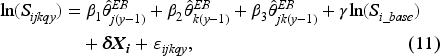
If OS and IS individual effects represent reps’ individual abilities and OS–IS synergistic effects reflect collaboration qualities, these effects should be able to predict customer sales. Therefore, we examined whether the effects estimated from the previous year are positively associated with customer sales in the next year. That is,

$$\begin{array}{rl}\text{ln}(S_{ijkqy})& ={\beta }_1{\hat{\theta }}_{j(y-1)}^{EB}+{\beta }_2{\hat{\theta }}_{k(y-1)}^{EB}+{\beta }_3{\hat{\theta }}_{jk(y-1)}^{EB}+\gamma \text{ln}(S_{i\mathrm{\_}base})\\ & +\mathit{\delta }{\mathit{X}}_{\mathit{i}}+{\epsilon }_{ijkqy},\end{array}$$

(11)

where $S_{ijkqy}$ is the customer sales in quarter q of year y, and ${\hat{\theta }}_{j(y-1)}^{EB}$ , ${\hat{\theta }}_{k(y-1)}^{EB}$ , and ${\hat{\theta }}_{jk(y-1)}^{EB}$ are the standardized empirical Bayes estimates from year y– 1. We z-score standardized the raw estimates of $\theta$ s (mean = 0, SD = 1) for convenient interpretation, with $S_{i\mathrm{\_}base}$ as the baseline sales evaluated at the beginning of year y, proxied by the sales in year y – 1 and y – 2, and ${\mathit{X}}_{\mathit{i}}$ including the same set of customer characteristics as in previous equations. Column 1 of Table 7 presents the estimation of equation (11). These results suggest that all three estimated effects can explain customer sales in the next year. The coefficient for ${\hat{\theta }}_{j(y-1)}^{EB}$ is positive and significant ( ${\beta }_1=$ .141, p < .01), suggesting 14.1% more revenue from a customer served by an OS with an individual effect of one SD above the mean, compared with an average OS. Similarly, the estimate of ${\hat{\theta }}_{k(y-1)}^{EB}$ effect ( ${\beta }_2$  = .087, p < .01) indicates 8.7% more revenue from a customer served by an IS with an individual effect of one SD above the mean; the estimate of ${\hat{\theta }}_{jk(y-1)}^{EB}$ ( ${\beta }_3=$ .130, p < .01) indicates 13.0% more revenue from a customer served by a dyad with synergistic effect one SD above the mean, compared with a dyad with an average synergistic effect.

Table 7.

Predicting future customer sales with value added metrics.

DV: $\text{ln}(S_{ijkqy})$	1	2	3	4	5	6
OS Individual effect $({\hat{\theta }}_{j(y-1)}$ )	0.141**	0.141**	0.141**	0.131**	0.137**	0.153**
	(0.007)	(0.007)	(0.008)	(0.007)	(0.010)	(0.008)
IS Individual effect $({\hat{\theta }}_{k(y-1)}$ )	0.087**	0.082**	0.078**	0.079**	0.090**	0.120**
	(0.007)	(0.007)	(0.008)	(0.007)	(0.011)	(0.008)
OS–IS synergistic effect $({\hat{\theta }}_{jk(y-1)}$ )	0.130**	0.120**	0.107**	0.131**	0.022*
	(0.008)	(0.008)	(0.008)	(0.008)	(0.011)
Lagged sales y−1	0.083**	0.084**	0.083**	0.083**	0.071**	0.084**
	(0.001)	(0.001)	(0.001)	(0.001)	(0.002)	(0.001)
Lagged sales y−2	0.041**	0.042**	0.042**	0.041**	0.009**	0.042**
	(0.001)	(0.001)	(0.001)	(0.001)	(0.002)	(0.001)
Customer relationship tenure	−0.061**	−0.062**	−0.069**	−0.069**	−0.158**	−0.068**
	(0.007)	(0.008)	(0.009)	(0.008)	(0.011)	(0.008)
National account dummy	0.147**	0.142**	0.137**	0.145**	0.076**	0.142**
	(0.014)	(0.015)	(0.016)	(0.015)	(0.021)	(0.015)
OS total sales at y−1						0.057**
						(0.011)
IS total sales at y−1						0.071**
						(0.010)
Industry dummies	Yes	Yes	Yes	Yes	Yes	Yes
Intercept	8.947**	8.949**	8.972**	10.255**	9.393**	8.886**
	(0.022)	(0.023)	(0.025)	(0.505)	(0.029)	(0.023)
N	68,611	62,415	51,978	68,611	19,667	68,611
R-square	0.276	0.271	0.261	0.278	0.199	0.269

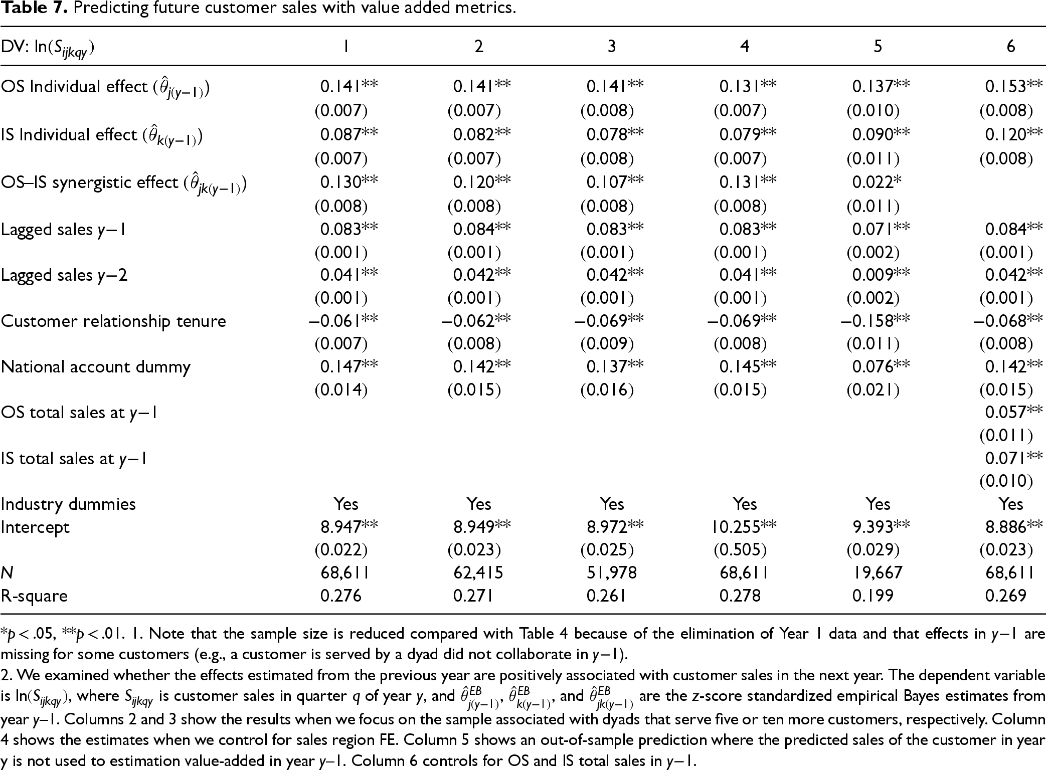
*p < .05, **p < .01. 1. Note that the sample size is reduced compared with Table 4 because of the elimination of Year 1 data and that effects in y−1 are missing for some customers (e.g., a customer is served by a dyad did not collaborate in y−1).

2. We examined whether the effects estimated from the previous year are positively associated with customer sales in the next year. The dependent variable is $\text{ln}(S_{ijkqy})$ , where $S_{ijkqy}$ is customer sales in quarter q of year y, and ${\hat{\theta }}_{j(y-1)}^{EB}$ , ${\hat{\theta }}_{k(y-1)}^{EB}$ , and ${\hat{\theta }}_{jk(y-1)}^{EB}$ are the z-score standardized empirical Bayes estimates from year y–1. Columns 2 and 3 show the results when we focus on the sample associated with dyads that serve five or ten more customers, respectively. Column 4 shows the estimates when we control for sales region FE. Column 5 shows an out-of-sample prediction where the predicted sales of the customer in year y is not used to estimation value-added in year y–1. Column 6 controls for OS and IS total sales in y−1.

The average SDs of the OS, IS, and interface synergistic effects for a year are .164, .110, and .134, respectively. These estimates suggest that increasing each effect by one SD from the average can generate 17.8% (OS), 11.6% (IS), and 14.3% (synergistic effect) ¹⁶ higher sales from an average customer. The effect size of the prediction is smaller but close to the raw estimates; 79.2% (OS), 75.0% (IS), and 90.9% (synergistic effect) ¹⁷ of the current year's estimated effects can be carried over to the following year, validating the conceptual and empirical consistency of our approach.

We next consider four sensitivity tests (Columns 2–5 of Table 7) and find stable predictive power of the estimated effects. Columns 2 and 3 show the results when we focus on the sample associated with dyads that serve five or 10 more customers, respectively. Column 4 of Table 7 provides the estimates when we control for sales region FE. Column 5 presents the predictability of OS, IS, and synergistic effects for customers that generate sales in year t but have no transactions in year y–1. Because we did not use these observations to estimate $\hat{\theta }$ in y–1, this analysis is an out-of-sample prediction. The predictive power of OS and IS individual effects at y–1 remains significant in predicting customer sales at t ( ${\beta }_1=$ .141, p < .01; ${\beta }_2=$ .090, p < .01), and that of synergistic effects is also positive and significant but smaller in magnitude ( ${\beta }_3=$ .022, p < .05).

6.6 Do Value-Added Metrics Perform Better Than Traditional Metrics?

The focal firm uses the total sales of customers served by a rep as its performance metrics. We assessed whether value-added metrics could predict customer sales better than traditional metrics. We z-score–standardized the log-transformed total sales that each OS and IS accumulates in year y–1 and used both the total sales and value added by OS and IS to predict customer sales in y. The value-added metrics predicted customer sales better than the total sales metrics. The coefficients of OS and IS total sales are .057 (p < .01) and .071 (p < .01), respectively, smaller than the coefficients of the OS (.153, p < .01) and IS (.120, p < .01) value-added metrics (Table 7, Column 6). Thus, value-added metrics indicate a useful alternative and supplement to existing performance evaluations.

6.7 Are Value-Added Metrics Associated with Customer Churn?

If the estimated effects reflect the selling quality of the reps and their interfaces, the value-added metrics should be correlated to customer churn. To test, we run the following probit model:

$$\begin{array}{rl}\text{Pr}(Chur{n}_{ijkqy}=1)& =\mathrm{\Phi }[{\rho }_1{\hat{\theta }}_{j(y-1)}^{EB}+{\rho }_2{\hat{\theta }}_{k(y-1)}^{EB}+{\rho }_3{\hat{\theta }}_{jk(y-1)}^{EB}\\ & +\gamma \text{ln}(S_{i\mathrm{\_}base})+\mathit{\delta }{\mathit{X}}_{\mathit{i}}+{\epsilon }_{ijkqy}\phantom{\frac{2}{1}}],\end{array}$$

(12)

where $\text{Pr}$ () is the probability of $Chur{n}_{ijkqy}$  = 1, and Φ represents the cumulative distribution function of the standard normal distribution. The focal company identifies customer churn when a customer remains inactive for one year. We set $Chur{n}_{ijkqy}$  = 1 when customer i at quarter q of year y has its last transaction within the subsequent year. The other notations were the same as in equation (11). We excluded customers who had transactions less than one year before the end of our data window, as we could not determine whether they had churned or not. Column 1 of Table 8 reports the results, showing that customer churn is driven mainly by OS individual effects. If the OS individual effect increases by one SD, the probability of customer churn decreases by .4%. This churn-reducing effect is more salient for national accounts (Column 2 of Table 8) than nonnational accounts (Column 3).

Table 8.

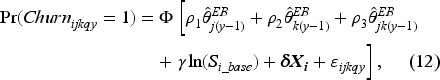
Associations between customer churn and value added metrics.

	1	2	3
OS individual effect $({\hat{\theta }}_{j(t-1)}$ )	−0.016*	−0.032**	−0.007
	(0.006)	(0.011)	(0.008)
IS individual effect $({\hat{\theta }}_{k(t-1)}$ )	0.004	−0.008	0.012
	(0.007)	(0.012)	(0.009)
OS–IS synergistic effect $({\hat{\theta }}_{jk(t-1)}$ )	−0.007	0.011	−0.016†
	(0.007)	(0.012)	(0.009)
Lagged sales t−1	−0.061**	−0.063**	−0.059**
	(0.001)	(0.002)	(0.002)
Lagged sales t−2	−0.045**	−0.052**	−0.041**
	(0.001)	(0.002)	(0.002)
Customer relationship tenure	−0.399**	−0.355**	−0.418**
	(0.008)	(0.013)	(0.009)
National account dummy	−0.099**
	(0.014)
Industry dummies	Yes	Yes	Yes
Intercept	0.977**	0.812**	0.988**
	(0.021)	(0.039)	(0.026)
N	57,168	23,292	33,876
Pseudo R-square	0.155	0.166	0.136

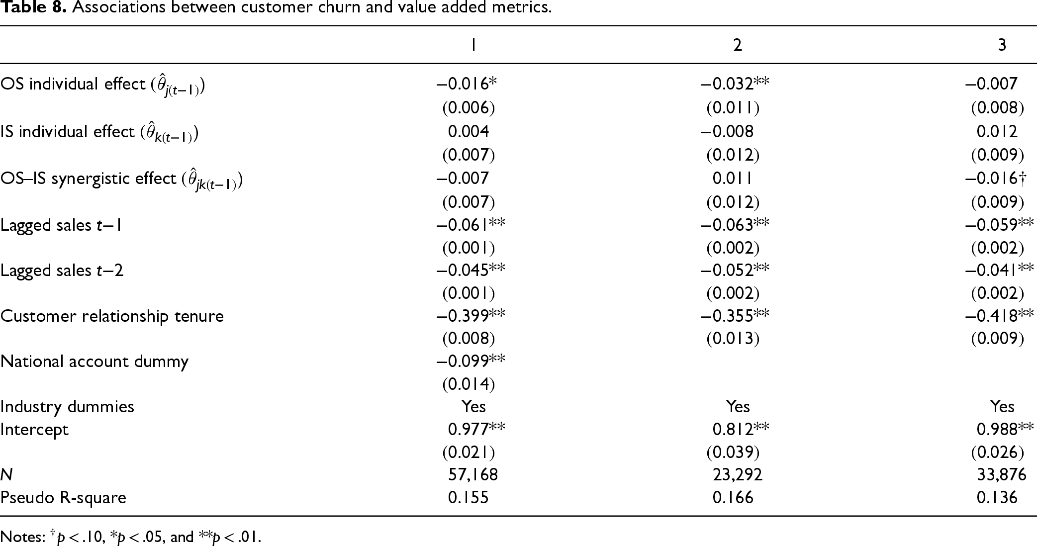
Notes: †p < .10, *p < .05, and **p < .01.

The evidence from Sections 6.5 to 6.7 demonstrates the predictive validity of the value-added metrics. Because the impact of value-added carries over to future customer sales, firms can use these metrics to improve the accuracy of their sales forecasts. Moreover, with 41% of churn interventions correctly targeted—compared to 23.4% under random targeting—firms can implement more efficient and effective retention strategies. ¹⁸

7 Additional Comparisons of FE and Empirical Bayes Estimates

Firms seeking to partition sales contributions may face varying degrees of uncertainty in customer purchases due to environmental shocks, unobserved customer hetergoneity, variations in OS–IS combinations, and diverse models for forming OS–IS teams. We will next compare the performance and sensitivity of FE and empirical Bayes estimations by examining these aspects.

7.1 Random Shocks and Unobserved Customer-Specific Heterogeneity Effects

Customer purchases may be affected by unobserved random shocks. To test the sensitivity of the value-partitioning approach, we adjust the standard deviation of the Gaussian distribution for $e_{ijkq}$ (mean = 0) to values of 0.1, 0.3, 0.5, 0.7, and 0.9, while keeping other parameters the same as the simulation in 6.3. Web Appendix H presents the results. Overall, empirical Bayes performs significantly better than FE estimation. For both methods, lower variability in unobserved random shocks results in lower bias, lower RMSE, and higher rank correlations. Even at a high shock level (0.9), empirical Bayes yields bias below 0.01, while FE produces bias exceeding 0.7.

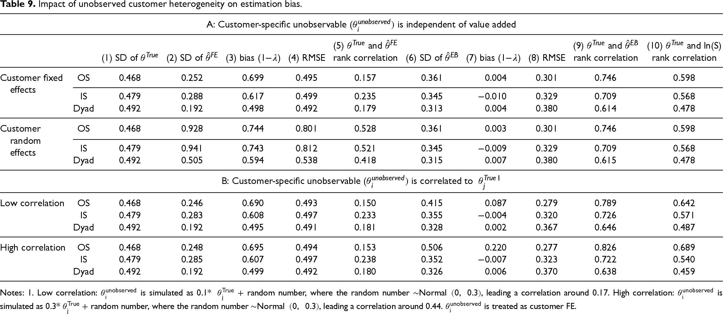
Customer-specific heterogeneity may not be fully captured by the observable characteristics firms collect. To assess the impact of unobserved customer heterogeneity, we modify the simulation in 6.3 by adding an unobserved customer-level component ${\theta }_i^{unobserved}\sim Normal\text{; }(0,\text{; }0.5)$ . We first test whether model performance varies under customer FE versus random effects, to isolate the influence of ${\theta }_i^{unobserved}$ on the estimation results. We find that empirical Bayes continues to perform significantly better than FE estimation (Table 9, Panel A), yielding similar results regardless of whether ${\theta }_i^{unobserved}$ is modeled as fixed or random effects. In contrast, FE is sensitive to the treatment of ${\theta }_i^{unobserved}$ ; compared to FE treatment of ${\theta }_i^{unobserved}$ , random effects treatment overestimates the variability of value-added and exhibits larger RMSEs. We next correlate ${\theta }_i^{unobserved}$ with the true value-added of OS rep ( ${\theta }_j^{True}$ ) and estimate ${\theta }_i^{unobserved}$ as FE. We find empirical Bayes remain superior to FE estimation (Table 9, Panel B). Due to the positive correlation between ${\theta }_i^{unobserved}$ and ${\theta }_j^{True}$ , both approaches tend to attribute part of the ${\theta }_i^{unobserved}$ to OS rep's estimated value added, resulting in a positive bias. However, the bias under empirical Bayes is only 12% to 31% of that produced by FE estimation. Notably, the rank-based performance metrics of empirical Bayes are unaffected by this correlation and remain superior to both FE and raw sales rankings. Similar patterns are observed when ${\theta }_i^{unobserved}$ is correlated with all three value-added components (see Web Appendix H).

Table 9.

Impact of unobserved customer heterogeneity on estimation bias.

A: Customer-specific unobservable ( ${\theta }_i^{unobserved})$ is independent of value added
		(1) SD of ${\theta }^{True}$	(2) SD of ${\hat{\theta }}^{FE}$	(3) bias (1 $-\lambda$ )	(4) RMSE	(5) ${\theta }^{True}$ and ${\hat{\theta }}^{FE}$ rank correlation	(6) SD of ${\hat{\theta }}^{EB}$	(7) bias (1 $-\lambda$ )	(8) RMSE	(9) ${\theta }^{True}$ and ${\hat{\theta }}^{EB}$ rank correlation	(10) ${\theta }^{True}$ and ln(S) rank correlation
Customer fixed effects	OS	0.468	0.252	0.699	0.495	0.157	0.361	0.004	0.301	0.746	0.598
	IS	0.479	0.288	0.617	0.499	0.235	0.345	−0.010	0.329	0.709	0.568
	Dyad	0.492	0.192	0.498	0.492	0.179	0.313	0.004	0.380	0.614	0.478
Customer random effects	OS	0.468	0.928	0.744	0.801	0.528	0.361	0.003	0.301	0.746	0.598
	IS	0.479	0.941	0.743	0.812	0.521	0.345	−0.009	0.329	0.709	0.568
	Dyad	0.492	0.505	0.594	0.538	0.418	0.315	0.007	0.380	0.615	0.478
B: Customer-specific unobservable ( ${\theta }_i^{unobserved})$ is correlated to ${\theta }_j^{True}$ 1
Low correlation	OS	0.468	0.246	0.690	0.493	0.150	0.415	0.087	0.279	0.789	0.642
	IS	0.479	0.283	0.608	0.497	0.233	0.355	−0.004	0.320	0.726	0.571
	Dyad	0.492	0.192	0.495	0.491	0.181	0.328	0.002	0.367	0.646	0.487
High correlation	OS	0.468	0.248	0.695	0.494	0.153	0.506	0.220	0.277	0.826	0.689
	IS	0.479	0.285	0.607	0.497	0.238	0.352	−0.007	0.323	0.722	0.540
	Dyad	0.492	0.192	0.499	0.492	0.180	0.326	0.006	0.370	0.638	0.459

Notes: 1. Low correlation: ${\theta }_{\text{i}}^{\text{unobserved}}$ is simulated as 0.1* ${\theta }_{\text{j}}^{\text{True}}$ + random number, where the random number $\sim \text{Normal; }(0,\text{; }0.3)$ , leading a correlation around 0.17. High correlation: ${\theta }_{\text{i}}^{\text{unobserved}}$ is simulated as 0.3* ${\theta }_{\text{j}}^{\text{True}}$ + random number, where the random number $\sim \text{Normal; }(0,\text{; }0.3)$ , leading a correlation around 0.44. ${\theta }_{\text{i}}^{\text{unobserved}}$ is treated as customer FE.

7.2 Variations of OS–IS Combinations

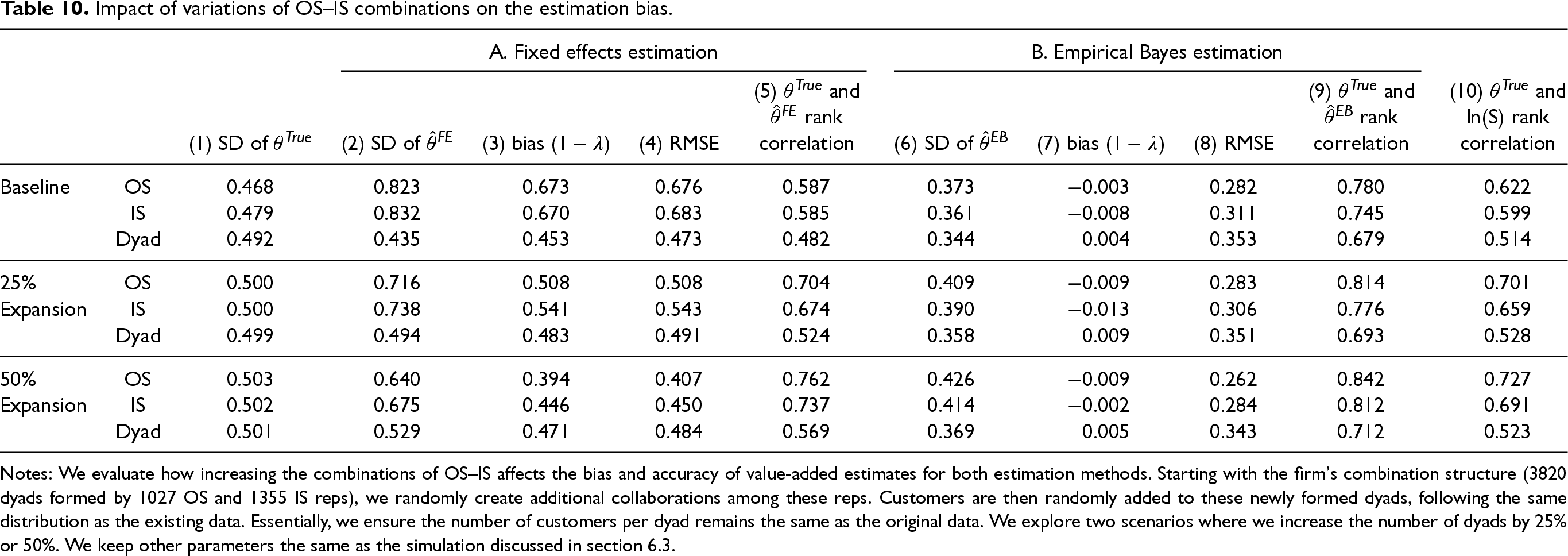
We next evaluate how increasing the combinations of OS–IS affects the bias and accuracy of value-added estimates for both estimation methods. Starting with the firm's combination structure (3820 dyads formed by 1027 OS and 1355 IS reps), we randomly create additional collaborations among these reps. Customers are then randomly added to these newly formed dyads, following the same distribution as the existing data. Essentially, we ensure the number of customers per dyad remains the same as the original data. We explore two scenarios where we increase the number of dyads by 25% o 50% (more scenarios in Web Appendix H). We keep other parameters the same as the simulation in 6.3.

The estimated results in Table 10 show that empirical Bayes estimation outperforms the FE estimation by producing much smaller biases and more accurate estimates in terms of RMSE and rank correlations. The increased diversity of OS–IS combinations reduces bias and improves the accuracy for all three types of value-added metrics and for both estimation methods. The increased diversity of combinations improves the FE estimation more significantly than its impact on the empirical Bayes.

Table 10.

Impact of variations of OS–IS combinations on the estimation bias.

			A. Fixed effects estimation				B. Empirical Bayes estimation
		(1) SD of ${\theta }^{True}$	(2) SD of ${\hat{\theta }}^{FE}$	(3) bias ( $1-\lambda$ )	(4) RMSE	(5) ${\theta }^{True}$ and ${\hat{\theta }}^{FE}$ rank correlation	(6) SD of ${\hat{\theta }}^{EB}$	(7) bias ( $1-\lambda$ )	(8) RMSE	(9) ${\theta }^{True}$ and ${\hat{\theta }}^{EB}$ rank correlation	(10) ${\theta }^{True}$ and ln(S) rank correlation
Baseline	OS	0.468	0.823	0.673	0.676	0.587	0.373	−0.003	0.282	0.780	0.622
	IS	0.479	0.832	0.670	0.683	0.585	0.361	−0.008	0.311	0.745	0.599
	Dyad	0.492	0.435	0.453	0.473	0.482	0.344	0.004	0.353	0.679	0.514
25%	OS	0.500	0.716	0.508	0.508	0.704	0.409	−0.009	0.283	0.814	0.701
Expansion	IS	0.500	0.738	0.541	0.543	0.674	0.390	−0.013	0.306	0.776	0.659
	Dyad	0.499	0.494	0.483	0.491	0.524	0.358	0.009	0.351	0.693	0.528
50%	OS	0.503	0.640	0.394	0.407	0.762	0.426	−0.009	0.262	0.842	0.727
Expansion	IS	0.502	0.675	0.446	0.450	0.737	0.414	−0.002	0.284	0.812	0.691
	Dyad	0.501	0.529	0.471	0.484	0.569	0.369	0.005	0.343	0.712	0.523

Notes: We evaluate how increasing the combinations of OS–IS affects the bias and accuracy of value-added estimates for both estimation methods. Starting with the firm's combination structure (3820 dyads formed by 1027 OS and 1355 IS reps), we randomly create additional collaborations among these reps. Customers are then randomly added to these newly formed dyads, following the same distribution as the existing data. Essentially, we ensure the number of customers per dyad remains the same as the original data. We explore two scenarios where we increase the number of dyads by 25% or 50%. We keep other parameters the same as the simulation discussed in section 6.3.

7.3 Positive Assortative Pairing

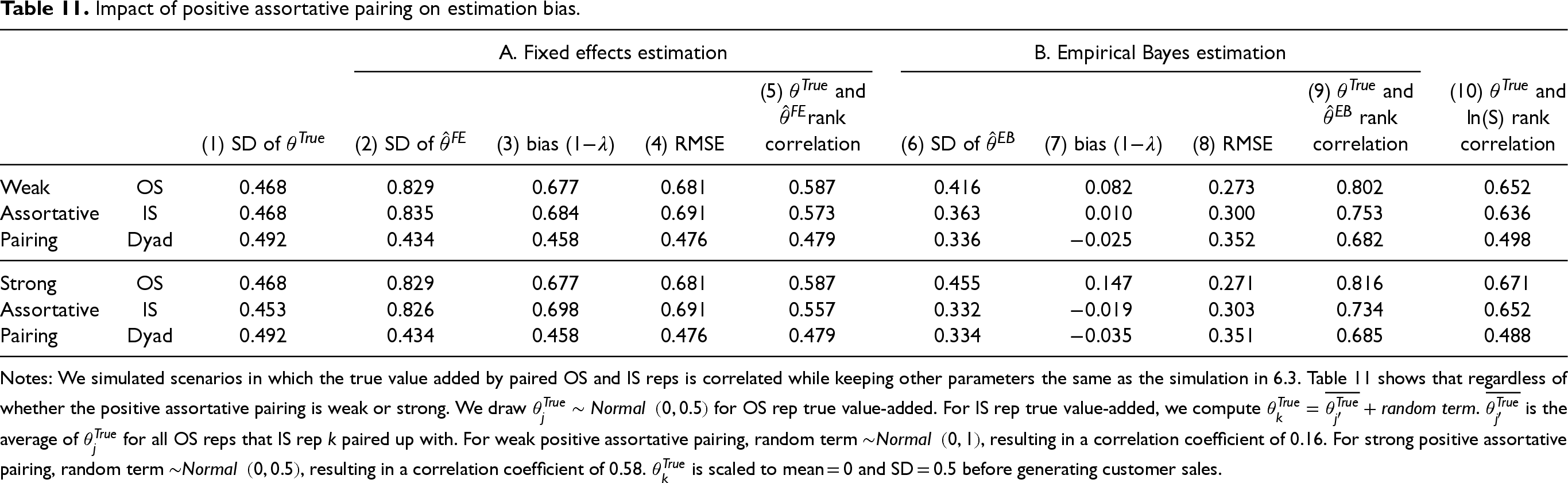
In some firms, reps may have the freedom to form collaborations voluntarily. A high-performing OS rep may prefer to form collaboration with high-performing IS reps. We simulated scenarios in which the true value added by paired OS and IS reps is correlated while keeping other parameters the same as the simulation in 6.3. Table 11 shows that regardless of whether the positive assortative pairing is weak or strong, ¹⁹ the empirical Bayes produces small and acceptable biases (−0.035 to 0.147), whereas FE estimation results in significant biases (0.458 to 0.698). Empirical Bayes also outperforms FE in terms of RMSE and rank correlations.

Table 11.

Impact of positive assortative pairing on estimation bias.

			A. Fixed effects estimation				B. Empirical Bayes estimation
		(1) SD of ${\theta }^{True}$	(2) SD of ${\hat{\theta }}^{FE}$	(3) bias (1 $-\lambda$ )	(4) RMSE	(5) ${\theta }^{True}$ and ${\hat{\theta }}^{FE}$ rank correlation	(6) SD of ${\hat{\theta }}^{EB}$	(7) bias (1 $-\lambda$ )	(8) RMSE	(9) ${\theta }^{True}$ and ${\hat{\theta }}^{EB}$ rank correlation	(10) ${\theta }^{True}$ and ln(S) rank correlation
Weak	OS	0.468	0.829	0.677	0.681	0.587	0.416	0.082	0.273	0.802	0.652
Assortative	IS	0.468	0.835	0.684	0.691	0.573	0.363	0.010	0.300	0.753	0.636
Pairing	Dyad	0.492	0.434	0.458	0.476	0.479	0.336	−0.025	0.352	0.682	0.498
Strong	OS	0.468	0.829	0.677	0.681	0.587	0.455	0.147	0.271	0.816	0.671
Assortative	IS	0.453	0.826	0.698	0.691	0.557	0.332	−0.019	0.303	0.734	0.652
Pairing	Dyad	0.492	0.434	0.458	0.476	0.479	0.334	−0.035	0.351	0.685	0.488

Notes: We simulated scenarios in which the true value added by paired OS and IS reps is correlated while keeping other parameters the same as the simulation in 6.3. Table 11 shows that regardless of whether the positive assortative pairing is weak or strong. We draw ${\theta }_j^{True}\sim Normal\text{; }(0,0.5)$ for OS rep true value-added. For IS rep true value-added, we compute ${\theta }_k^{True}=\overline{{\theta }_{j{}^{\mathrm{\prime }}}^{True}}+randomterm$ . $\overline{{\theta }_{j{}^{\mathrm{\prime }}}^{True}}$ is the average of ${\theta }_j^{True}$ for all OS reps that IS rep k paired up with. For weak positive assortative pairing, random term $\sim Normal\text{; }(0,1)$ , resulting in a correlation coefficient of 0.16. For strong positive assortative pairing, random term $\sim Normal\text{; }(0,0.5)$ , resulting in a correlation coefficient of 0.58. ${\theta }_k^{True}$ is scaled to mean = 0 and SD = 0.5 before generating customer sales.

7.4 Positive Assortative Pairing and Endogenous Synergistic Effects

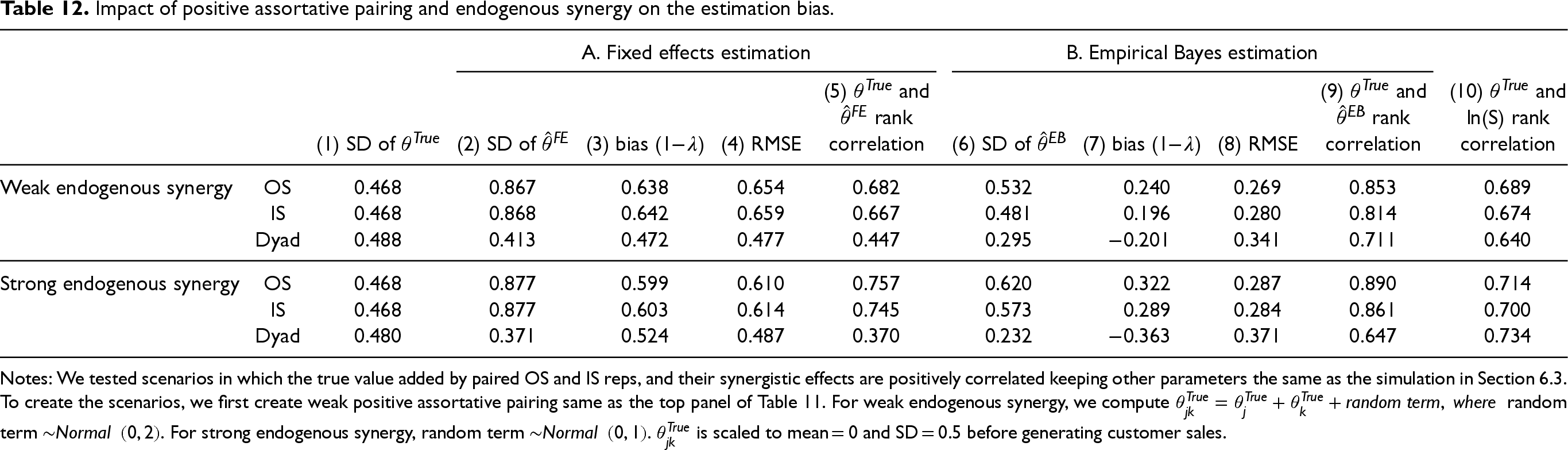
Collaboration between similar individuals is likely to be more effective and cohesive, resulting in higher synergistic effects. We simulated scenarios in which the true value added by paired OS and IS reps, and their synergistic effects are positively correlated keeping other parameters the same as the simulation in 6.3. ²⁰ Table 12 shows while empirical Bayes overall still perform better than FE, both estimation methods produce sizable biases (Columns 3 and 7). Rank correlations indicate that empirical Bayes estimates preserve the true value-added order for individual effects more accurately than FE estimation and joint sales outcome. However, both estimations fail to preserve the order of synergistic effects.

Table 12.

Impact of positive assortative pairing and endogenous synergy on the estimation bias.

			A. Fixed effects estimation				B. Empirical Bayes estimation
		(1) SD of ${\theta }^{True}$	(2) SD of ${\hat{\theta }}^{FE}$	(3) bias (1 $-\lambda$ )	(4) RMSE	(5) ${\theta }^{True}$ and ${\hat{\theta }}^{FE}$ rank correlation	(6) SD of ${\hat{\theta }}^{EB}$	(7) bias (1 $-\lambda$ )	(8) RMSE	(9) ${\theta }^{True}$ and ${\hat{\theta }}^{EB}$ rank correlation	(10) ${\theta }^{True}$ and ln(S) rank correlation
Weak endogenous synergy	OS	0.468	0.867	0.638	0.654	0.682	0.532	0.240	0.269	0.853	0.689
	IS	0.468	0.868	0.642	0.659	0.667	0.481	0.196	0.280	0.814	0.674
	Dyad	0.488	0.413	0.472	0.477	0.447	0.295	−0.201	0.341	0.711	0.640
Strong endogenous synergy	OS	0.468	0.877	0.599	0.610	0.757	0.620	0.322	0.287	0.890	0.714
	IS	0.468	0.877	0.603	0.614	0.745	0.573	0.289	0.284	0.861	0.700
	Dyad	0.480	0.371	0.524	0.487	0.370	0.232	−0.363	0.371	0.647	0.734

Notes: We tested scenarios in which the true value added by paired OS and IS reps, and their synergistic effects are positively correlated keeping other parameters the same as the simulation in Section 6.3.

To create the scenarios, we first create weak positive assortative pairing same as the top panel of Table 11. For weak endogenous synergy, we compute ${\theta }_{jk}^{True}={\theta }_j^{True}+{\theta }_k^{True}+randomterm,where$ random term $\sim Normal\text{; }(0,2)$ . For strong endogenous synergy, random term $\sim Normal\text{; }(0,1)$ . ${\theta }_{jk}^{True}$ is scaled to mean = 0 and SD = 0.5 before generating customer sales.

8 Discussion

With this research, we propose a value-partitioning approach that separates joint sales contributions into individual value-added components. Our application to a B2B company demonstrates the managerial value of this approach. Additionally, a series of simulations show that empirical Bayes estimation outperforms FE estimation, especially when facing the challenges of sparse OS–IS combinations.

8.1 Implications for Sales Organizations and Researchers

The value-added metrics offer valuable applications for sales organizations and researchers, offering novel ways to evaluate sales interventions and understand the underlying drivers of sales performance.

One key application is assessing the impact of sales programs or interventions. As introduced in the Introduction and detailed in Web Appendix A (A3), ABC Firm sought to refine the features of its recently launched sales automation platform, primarily used by IS reps. In a pre and post with control group design, by comparing the rankings of IS value-added and interface value-added before and after the platform's implementation—between IS reps who were randomly selected to use the platform and those who were not—firms can evaluate its impact on both IS reps’ individual contributions and their collaborative interactions with OS reps.

As demonstrated in the use case (with implementation coding), ABC Firm found that while the platform improved IS reps’ value-added, it unintentionally weakened the value-added of their interactions with OS reps. This insight suggests that the firm should prioritize features that strengthen interactions between IS and OS reps to ensure that technology adoption enhances, rather than disrupts, cross role interactions. Without value-partitioning, ABC would need to conduct a factorial experimental design, which is often infeasible given the large number of sales reps and dyads involved.

A second important application is identifying the key drivers of sales contributions. Managers and researchers can leverage value-added metrics to examine how different salesperson attributes influence performance. By linking these metrics to observable characteristics, firms can uncover important patterns in their salesforce data. For instance, in the focal firm, regressing value-added metrics on rep tenure and the number of industries a rep served revealed that tenure was positively associated with value-added, suggesting that experience enhances a salesperson's ability to generate value. Conversely, reps engaged across multiple industries exhibited lower value-added, indicating that specialization within a specific industry may lead to higher performance (detailed in Web Appendix H). These insights enable firms to make informed decisions about hiring, training, and team structuring to maximize sales effectiveness.

For sales researchers, the ability to isolate individual contributions and synergistic effects within sales teams provides a more nuanced understanding of how interventions and personal attributes influence outcomes. Future research could extend these insights by exploring additional contextual factors, such as customer characteristics, incentive structures, and evolving sales technologies. By integrating value-added metrics into sales research, scholars can develop more precise models that bridge theory and practice, ultimately advancing both academic knowledge and managerial decision-making.

8.2 Generalizability and Limitations

The value-partitioning approach can be applied to production process involving multiple roles where the joint outcome is observable. For example, teams composed of personnel from multiple departments (e.g., R&D, sales, and technical specialists) serve key account customers. The key requirement for the method is sufficient variation in the combinations of the roles for the model to reliably separate individual and synergistic effects. ²¹ In the focal firm, each OS rep collaborates with 3–4 IS reps and vice versa. However, collaboration structures can vary across industries. For example, in industries with highly specialized sales roles, such as enterprise software or medical devices, role collaborations may be more frequent, leading to denser interactions. Conversely, in industries with more independent sales operations, such as real estate or insurance, cross-role interactions may be sparser. To help sales organizations and researchers apply this approach across different contexts, we have developed a general application procedure (Web Appendix A), outlined in a structured flowchart that details the essential steps and necessary modifications.

In the implementation procedure, we outline several aspects that firms can adapt to align the approach with their own sales process characteristics. One critical decision for sales organizations and researchers is selecting the covariates to include in the model, as the sales impact of these variables will not be attributed to value-added metrics. A key element is sales baseline, which serves as a proxy for what an existing customer would likely purchase without any sales effort. For the focal firm, we used lagged sales as the proxy, as the sales cycle is shorter than the annual evaluation period. However, for industries with longer sales cycles (e.g., machinery, industrial equipment), firms may need to track past service contracts, maintenance agreements, or spare part purchases to construct a reliable baseline proxy. In mixed sales models (e.g., solutions-based businesses), firms may need to establish different baseline proxies for distinct revenue streams, such as one-time hardware purchases, recurring software subscriptions, or aftermarket services (e.g., training, upgrades, or customizations), to accurately reflect customer purchasing behavior across different types of sales interactions.

Our study has several limitations. First, we focus on partitioning value added in the relationship maintenance stage, so our findings apply to sales reps’ effects in this context. Future research could examine how these effects differ during customer acquisition. Applying our approach to acquisition data, where failed attempts are observable, could provide a more holistic view of OS, IS, and their interfaces.

Second, industry characteristics, sales models, and operating environments may impact data quality and value-added estimation. For instance, in in-store retail sales, contributions from team members may go unrecorded due to the lack of sales rep identifiers, making value-added estimation inaccurate or infeasible. Firms with stable teams over extended periods may see both individual and synergistic value-added increase over time. In such cases, caution is needed when the two types of effects are highly correlated, as both estimation methods may produce biased estimates, and firms may need to rely on value-added rankings for sales program evaluations.

Supplemental Material

sj-docx-1-pao-10.1177_10591478251340433 - Supplemental material for Value-Partitioning of Sales Contribution in Business Markets

Supplemental material, sj-docx-1-pao-10.1177_10591478251340433 for Value-Partitioning of Sales Contribution in Business Markets by Huanhuan Shi, Shrihari Sridhar and Rajdeep Grewal in Production and Operations Management