
Abstract
Modern decision-support applications build on planning parameters such as lead time, price, yield, etc., which are maintained as master data. The accuracy of master data significantly influences the viability of such applications. However, the maintenance of master data is considered a tedious and error-prone task. In this study, we explore the effectiveness of machine learning techniques to improve the accuracy of plan lead times. We apply both unsupervised and supervised learning methods for creating lead time prediction models. We test our approach using historical data of a global equipment manufacturer. In a numerical analysis the calculated plan lead times are over 30% more accurate than current plan lead times in terms of mean-squared-error (MSE). This increased accuracy of plan lead times reduces inventory investment by approximately 7%.
Introduction
Supply chain management has become an integral factor in competitive strategy to enhance organizational productivity and profitability (Li et al., 2006). Considerable research and effort have been devoted to formulating optimization methods that require master data to achieve high quality results. Maintenance of master data is a time-consuming, tedious and error prone task since the data can be volatile, ambiguous, and influenced by factors outside the company’s scope (Escudero et al., 1999).
Artificial intelligence (AI) technologies have gained prominence in their application to business-related problems and have been applied to pattern recognition, inference and learning from experience (Brynjolfsson and McAfee, 2017). In supply chain management, AI applications have been developed and deployed to, for example, inventory control and planning, transportation network planning, and purchasing and supply management (Min, 2010).
This study is motivated by a problem faced by a global equipment manufacturer which we refer to as “the company.” The company has annual sales of several billion euros and operates world-wide. To provide maintenance and repair services for specialized equipment, the service department holds spare parts in stock. While some stock-keeping-units (SKU) are produced internally, many are purchased from external suppliers with different lead times. To coordinate inventory levels across multiple levels in their supply chain, the company employs optimization methods for determining inventory control parameters, that is re-order points, base-stock levels and order quantities. The calculation of these parameters relies on plan lead times that are retrieved from their enterprise resource planning (ERP) system. Due to inaccurate plan lead times of some SKUs, many inventory control parameters are sub-optimal, resulting in lower service levels or higher inventory than optimal.
In this article, we address plan lead times and analyze how well their accuracy can be improved by machine learning. We propose a method to derive plan lead times with machine learning and compare the performance of three different machine learning regression algorithms: linear regression, random forests, and gradient boosting. We benchmark their performance with classical statistical approaches, that is single-exponential-smoothing (SES) and the historical average, as well as the current plan lead times from the company’s ERP system.
Our results show that plan lead times estimated with machine learning predict lead times more accurately than currently employed plan lead times. The best performing machine learning model improves lead time accuracy in terms of MSE by over 30% compared to current plan lead times. We also analyze the accuracy of our method for SKUs with respect to their procurement frequency and we find that our approach offers significant gains even for newly sourced SKUs. For very frequently procured SKUs, our approach still offers substantial gains in accuracy compared to classical statistical measures, but the difference is smaller than for infrequently procured SKUs.
To quantify the expected business benefits from improved plan lead times, we conducted an inventory simulation on historical data. The results from the simulation show that inventory holding can be reduced by approximately 7% while maintaining the same service level.
The remainder of this paper is structured as follows. In Section 2, we review the relevant literature on lead time prediction. In Section 3, we outline the problem and identify requirements for improving plan lead times with machine learning. In Section 4, we present our method of both supervised and unsupervised learning. In Section 5, we examine the economic implications of improved plan lead times and present numerical results. In Section 6, we derive practical implications, outline limitations and conclude.
Literature Review
Lead times are an important parameter in inventory optimization, extensively discussed in literature (Muthuraman et al., 2015; Silver et al., 2016; Wang, 2012). However, the literature has paid little attention to analyzing lead time accuracy and predicting lead times, especially in the context of inventory planning and optimization.
In practice, plan lead times are often derived from supply chain contracts, employee experience, or computed from historical data (Grout and Christy, 1993; Lawrenson, 1986; Lingitz et al., 2018; Urban, 2009). In some papers, lead times are predicted but not for stock replenishment. Berlec et al. (2008) examine how to accurately predict product delivery times, a critical factor in effective contract negotiations. Their study focuses on identifying commitment-worthy lead times for customers, ensuring that contracts reflect achievable delivery schedules. Similarly, Duffie et al. (2017) and Yang and Geunes (2007) explore aspects of customer lead time within contractual contexts, they do not specifically address its prediction for inventory replenishment.
Some recent studies have made promising strides in the field of lead time prediction through analytics. While these explorations are noteworthy, they present opportunities for further refinement and validation within the peer-reviewed scholarly community. Banerjee et al. (2015) combine matrix gamma distribution and step-wise linear regression to predict lead times. de Oliveira et al. (2021); Liu et al. (2018) employ regression models and compare various machine learning techniques, demonstrating high accuracy in predicting supplier lead times. However, these studies do not address the unique challenges in inventory management posed by spare parts, which are seldom re-ordered, leading to scarcity in historical data at the SKU level. These studies also neither address implementation of the approaches nor the financial implications of implementing such predictive models.
To address these gaps, our research leverages machine learning for lead time prediction. Insights from studies in related domains, such as transportation (Barbour et al., 2018; Choi et al., 2016; Hofleitner et al., 2012) and manufacturing (Bender and Ovtcharova, 2021; Burggräf et al., 2020; Lingitz et al., 2018), indicate the effectiveness of ensemble decision tree models. Specifically, the studies by Bender and Ovtcharova (2021); Gyulai et al. (2018); Lingitz et al. (2018); Oeztürk et al. (2006) have consistently demonstrated the superior performance of ensemble decision tree models such as random forest and gradient boosting in predicting various lead times.
While the existing literature offers insights into prediction methodologies, several open questions remain regarding how these predictions can be leveraged to derive accurate plan lead times for inventory control. Existing research focuses on predicting lead times at the individual purchase order level, whereas inventory control requires a lead time parameter to estimate the lead time demand distribution to compute base stock levels, safety stock or reorder points. This gap between order-level lead time predictions and the need for suitable parameters for inventory management is addressed in this article.
Moreover, while the literature addresses how lead time variability impacts base stock levels and inventory investments, it is typically assumed that the lead time distribution is already known or can be estimated from historical data. This assumption is particularly problematic for spare parts, where data is often sparse, making it difficult to estimate moments from historical observations.
Building on existing research in lead time prediction, we extend the literature by examining how varying SKU order frequencies affect bias in predictive models. The inherent bias introduced by SKU order frequency discrepancies presents a key challenge in procurement operations. Frequently ordered SKUs generate extensive historical data, allowing for higher prediction accuracy in machine learning models. Conversely, infrequently ordered SKUs have sparse historical data, leading to greater uncertainty in lead time predictions. This imbalance reflects the operational nature of procurement systems, where demand varies widely among SKUs. We address this challenge through a comprehensive approach combining feature engineering techniques and systematic evaluation of balancing methods for regression tasks.
Building on these findings, our analysis focuses on three machine learning models: linear regression, random forest, and gradient boosting (Breiman, 2001; Friedman, 2002; Weisberg, 2005). By applying these models to predict supplier lead times accurately, we aim to develop a framework that not only enhances inventory planning and optimization but also addresses the unique challenges posed by spare parts, thus contributing significantly to the existing body of knowledge in the field.
Problem Description
To offer repair and maintenance services to its customers, the company operates a warehouse network for its spare parts. To efficiently manage inventories, the service division of the company regularly optimizes its inventory control parameters (such as re-order points and base-stock levels) under service-level constraints. Due to inaccurate lead time parameters, inventory levels have been sub-optimal.
When analyzing the historical lead times, we observe a high dispersion. Figure 1 provides some information on lead times at the company. This data and other data of the company had to be sanitized by the company’s request, but the general insights and relative performance data that we report are not affected by the sanitation. Figure 1(a) shows the lead time distribution of all SKUs. We can see that the distribution is highly skewed with a long right tail. Figure 1(b) plots order frequencies against procurement lead times. While procurements with longer lead times generally belong to SKUs with lower order frequencies, no strong relationship exists between these variables. This is evidenced by a single SKU ordered approximately 280 times spanning lead times from 20 to 170 days. Figure 1(c) shows the accuracy of current plan lead times. We can see that the deviations from the planned lead times occur with similar magnitude in both directions. Figure 1(d) shows the order frequency of all SKUs. We find a highly skewed number of purchase orders per SKU. While a few SKUs are ordered at a high frequency, the majority of SKUs are ordered infrequently.
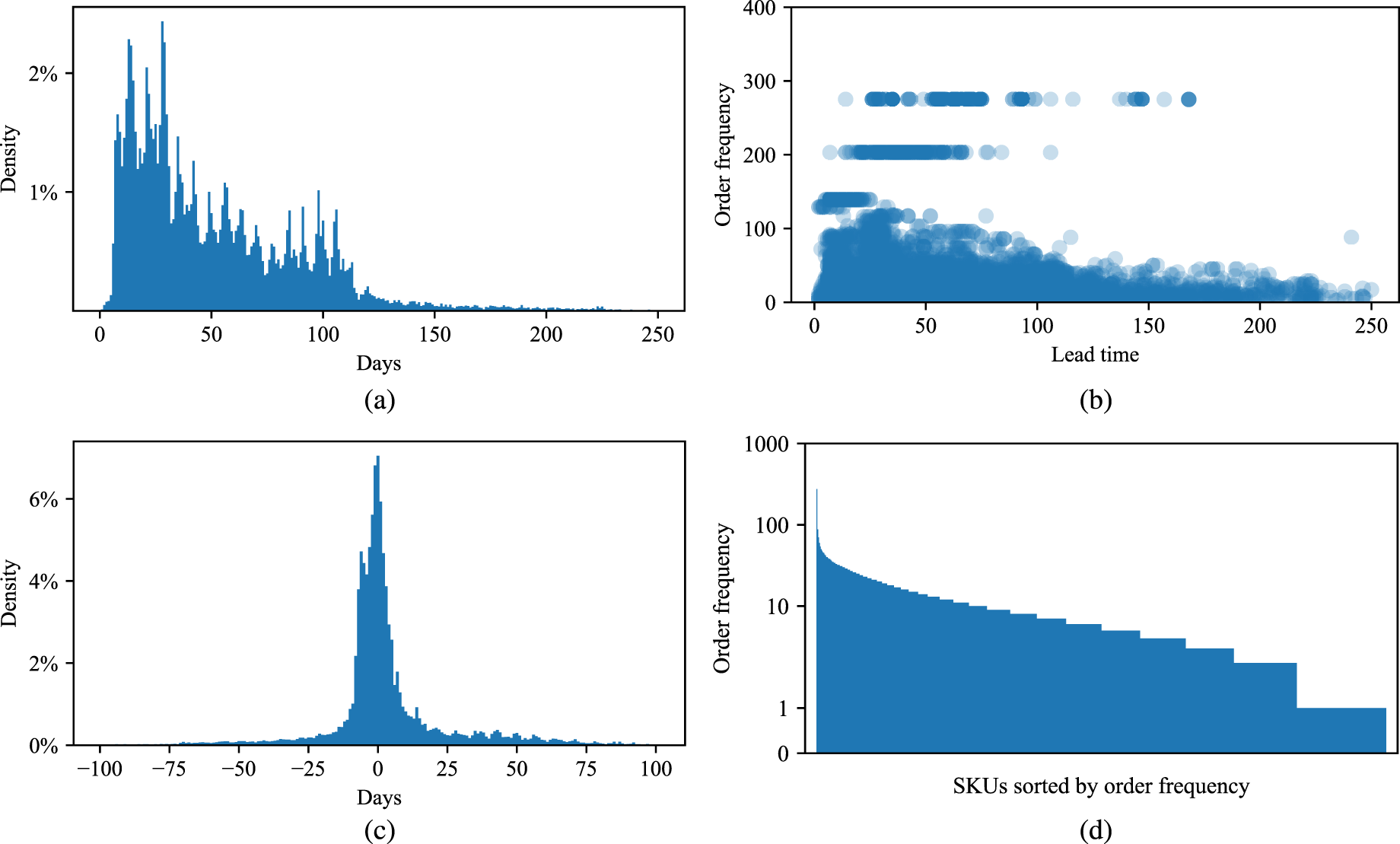
Plan and actual lead time characteristics of all purchase orders: (a) lead time dispersion; (b) order frequency against lead time; (c) plan lead time accuracy; (d) SKU order frequency.
Plan lead times are maintained as master data. These plan lead times are static and are rarely updated. The vendor management and the inventory management teams manage and maintain the plan lead times on the basis of the contractually agreed lead times. For most SKUs, the plan lead time is agreed upon with the individual supplier. For the remaining SKUs, the plan lead times are generated by calculating the historical average lead times of the SKU. Considering how infrequently most SKUs are procured, estimates based solely on historical lead time data (interpolation) are limited by the available observations. Together with experts from the company, we discussed which data from their ERP might contain causal information about lead times. After this qualitative approach, we queried operational attributes from the ERP system. We worked with two different data sources: SKU master data and transactional purchase order data.
Our methodology is structured into three fundamental stages. The first stage involves a rigorous data preparation process. We briefly touch our cleaning and merging process of the raw data sets, ensuring the integrity of the data. Subsequently, we conduct an insightful initial analysis to identify features with potential significance for our predictive models. The second stage encompasses feature engineering. This step is dedicated to the creation and transformation of features to improve the performance of the applied machine learning techniques. In the final stage we build upon the prepared data set and apply machine learning algorithms to refine our predictive models. We define robust evaluation techniques, serving as benchmarks for comparing and selecting the most effective models. Through regularization and hyper-parameter optimization, we tailor the models to predict plan lead times accurately.
Data Preparation and Exploratory Analysis
We work with two different data sources: SKU master data and transactional purchase order data. SKU master data contain data such as the supplier from which the SKU is sourced, the country it is sourced from, and the current plan lead time. Transactional purchase data contain information on purchased SKUs over four years (2018–2021), including the request and delivery date and the plan lead time at the time when the SKU was ordered. Therefore, this data set holds information on how master data, such as plan lead time, has changed over time.
Most pre-processing of our data consisted of storing information as correct data types and identifying SKUs with missing entries. Since we could not fix missing values, these SKUs representing less then 2% of the total data set were dropped.
An analysis of categorical variables reveals that a large share of purchase orders is sourced from the country in which the global warehouse is located (Figure EC.3). We also observe countries of origin with only few purchase orders and therefore we clustered countries from the same continent with less than 1% of the order volume. The remaining categorical variables seem plausible and do not require further processing.
While assessing the numerical features of our data sets, we observe some extreme outliers for the variable’s valuation price and purchase order quantity. We decide to winsorize them based on Tukey’s rule of thumb (Tukey, 1992). This method is widely used in statistical analysis (Carling, 2000; Wiley and Wiley, 2019) and applied in machine learning to ensure models account for all data points while mitigating the impact of extremes, where models benefit from capturing the full range of data without being skewed by extremes. It identifies outlier values based on the inter-quartile range (IQR). Corresponding outliers are truncated and set to a constant value equal to the IQR times a factor, which, following Tukey’s rule, we set to 1.5. For linear regression, we normalize numerical data by re-scaling features to the range of zero to one. We do not normalize the numerical data for random forest and gradient boosting, as tree based models do not require feature scaling (Brownlee, 2020).
Despite initial concerns about the potential impact of COVID-19 on lead-time volatility, our analysis did not uncover any significant fluctuations or patterns in the data, as illustrated in Figure 2. The lead times remain relatively stable over the observed period, with no extreme variances that would necessitate adjustments to the data set.
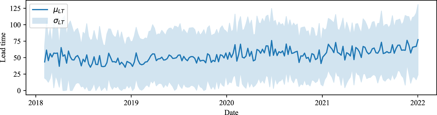
Lead time volatility over time.
Our final data set includes 160,048 purchase orders across 17,728 SKUs, which are used for model training and testing (cf. Table 1). For performance evaluation, we implement a fixed origin evaluation procedure, splitting the data into a training set and a test set (Tashman, 2000). The first 42 months of data comprise the training set, while the final 6 months, selected to coincide with the company’s semi-annual review period, form the test set.
Pre-processed features.
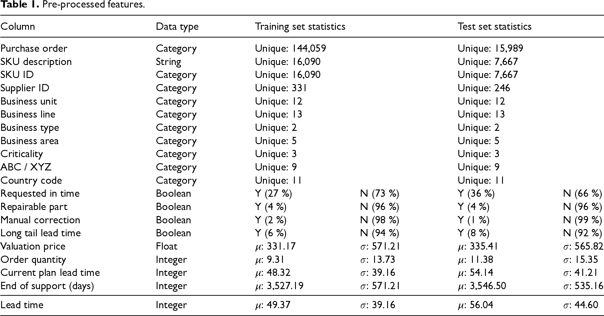
To validate that the data of the training set do not deviate heavily from the test set, we compare both sets in Table 1. Key statistics of all features for each set indicate that both share similar characteristics.
Although the overall lead time volatility remains relatively consistent over time, we observe an increase of 6.67 days in average lead times compared to the training set. This shift does not indicate a broader pattern but rather reflects normal operational variations. We explored various splitting points as suggested by Hyndman and Athanasopoulos (2018), but ultimately, we chose the above mentioned split to maintain sufficient observations. We exercise the train-test split at this point to ensure that no information from the test set is used for feature engineering.
We next present feature engineering techniques to extract meaningful information from the existing data set and to transform this information so that machine learning models can process it.
In our data set, we have short descriptions of the SKUs. We anticipate that our models can learn from other SKUs with similar lead times. For example, electronic parts with a similar description of “8 GB DDR4 RAM” and “16 GB DDR4 Memory” can have similar lead times.
Strings cannot be interpreted by machine learning algorithms and we must convert them into ratio scale numeric representations that machine learning algorithms can process. We use KNN-regression to identify similar SKUs from the same supplier based on their description (unsupervised learning). For each SKU, we calculate a measure of lead time central tendency from its similar SKUs and use it as a feature for the machine learning algorithm.
Before starting with feature engineering, we have to pre-process some data. Because the SKU descriptions are not very extensive, most data cleaning, like removing stop words or expanding contractions, is redundant (Webster and Kit, 1992). We merely remove extra white spaces, lowercase all characters, and split the descriptions into single words (tokenization).
Because the SKU descriptions are concise, we use the bag of words count vectorizer, a vector space representation model for unstructured text (Zhang et al., 2010). From a total of
Example count vectorization.
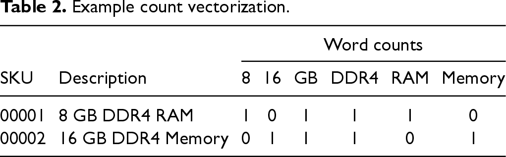
Example count vectorization.
We cluster SKUs which are sourced from the same supplier based on their cosine similarity. To evaluate if these clusters are meaningful to predict lead times, we analyze if SKUs from the same group have similar lead times. The part descriptions of the SKUs shown in Table 2, for example, have a cosine similarity of 0.83. For each SKU, we calculate its average lead time and compare it to the average of all historical lead times from the SKUs in the same cluster (cf. Figure 3(b)). We see that the average lead time of an SKU correlates with the average lead time of the SKUs from the same group. Therefore, we add the average lead time from the clustered SKUs as an additional feature. For SKUs which are not in any cluster, we take their average historical lead time. For those SKUs that have not been procured before we take the average lead times from the corresponding supplier.
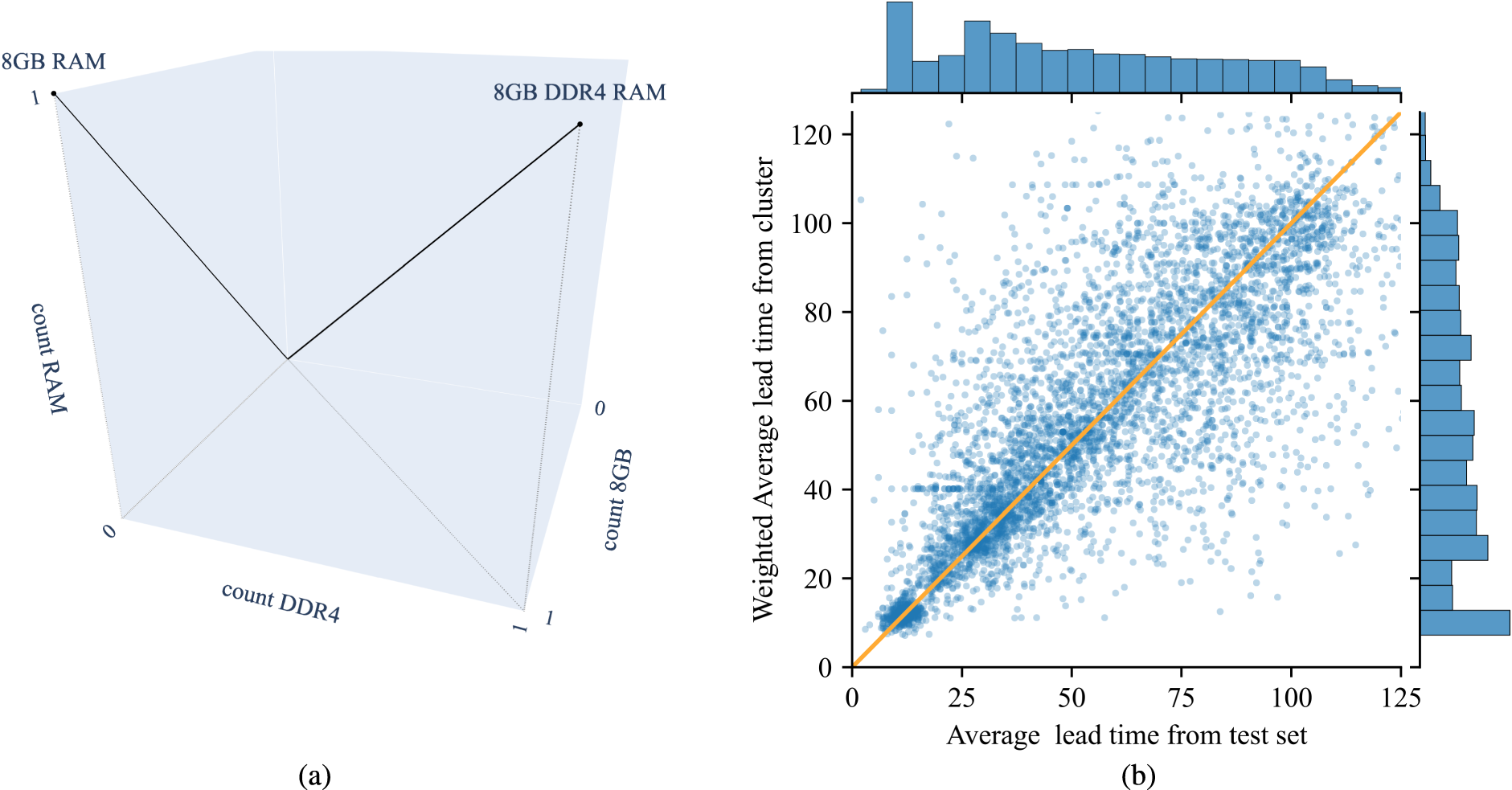
Creation of similarity feature: (a) 3D vector space cosine similarity; (b) average lead time correlation between SKU and cluster.
As shown in Figure 1(a), the distribution of the target variable (lead time) is skewed, indicating an imbalance with a long tail extending towards longer lead times. To address this, we explore various balancing techniques such as random over- and under-sampling, as well as synthetic minority oversampling for regression, which have been proposed for handling imbalanced regression tasks (Branco et al., 2017; Torgo et al., 2013). In our analysis, these sampling methods do not improve results, probably because such techniques are more suited for contexts where the under-represented numeric value interval is most critical, and a wrongful prediction can be costly, often at the expense of overall performance (Torgo et al., 2013).
Conducting a point-biserial correlation analysis, we find a weak but significant negative correlation
As an additional feature, we compute a measure of supplier performance according to the business rules applied at the company. At the company, the supplier performance is measured as the share of orders delivered in time compared to all orders placed at the supplier. We first compute this measure for each supplier in the training set. Afterwards, we append this measure to the corresponding supplier in the test set. Some suppliers included in the test set do not appear in the training set. For those, we take the average supplier performance across all suppliers in the training set to complete the records.
As in most machine learning applications, the target variable is influenced by categorical (nominal scale) features. One-hot encoding, the most widely used coding scheme (Rodríguez et al., 2018), but in our case leads to undesirable sparsity in the data, especially with numerous categories such as the supplier ID (Gupta and Asha, 2020; Prokhorenkova et al., 2017). To address this, we implement multiple Bayesian encoding techniques: target encoder, polynomial encoder, Helmert encoder, James-Stein encoder, m-estimate encoder, weight of evidence encoder and catboost encoder—for a full reference, please refer to Pedregosa et al. (2011); Prokhorenkova et al. (2017). We choose the one which performs best in cross-validation, an approach that we cover in the next section.
Informed by our literature review, we train three established machine learning algorithms to predict lead times: linear regression, random forest, and gradient boosting. Linear regression serves as our baseline, leveraging its capacity for modeling relationships between scalar responses and explanatory variables through a least squares approach (Weisberg, 2005). The random forest algorithm, aggregates predictions from a multitude of decision trees trained in parallel on random data subsets to enhance predictive accuracy and mitigate over-fitting (Breiman, 2001). Gradient boosting constructs an additive model in a forward stage-wise fashion, and is particularly adept at addressing the residuals of preceding trees, sharpening accuracy on more complex or noisy data sets (Friedman, 2002).
Our primary performance metric is the MSE as the performance of an inventory control system heavily depends on achieving a low MSE in lead time demand forecasts (Syntetos et al., 2009). The MSE penalizes large deviations from observations disproportionately compared to minor deviations.
However, we recognize that the MSE can be challenging to interpret due to its dependence on the scale of lead time, especially when assessments are conducted across various SKUs. To address this, we also report the mean-absolute-percentage-error (MAPE), a scale-free metric, which prevents high or low performance in terms of MSE from being disproportionately influenced by a few SKUs. In addition to MSE and MAPE, we also evaluate the bias (mean forecast error). Evaluating bias is crucial because even with high accuracy, a model that consistently over- or underestimates can lead to poor inventory performance.
As discussed in Section 3, the procurement frequency of SKUs in our dataset is highly skewed, potentially leading to bias for infrequently ordered items. To address this, we explore balancing techniques such as minority over-sampling (OS) and majority under-sampling (US), as well as sample weighting based on the inverse of order frequency. These methods aim for a more balanced representation of SKUs and try to improve the model’s ability to generalize across both frequently and infrequently ordered items. However, our results indicate that these techniques do not consistently improve model performance or significantly reduce bias. Therefore, we do not use these methods in the main analysis. Detailed results from the experiments are provided in Table EC.2 of the e-companion for reference and transparency.
To determine the effectiveness of these techniques, as well as to optimize hyper-parameters and perform feature elimination, we calibrate our models using a cross-validation procedure based on a rolling forecasting origin, applied to the training data (Hyndman, 2014). This technique takes into account the temporal nature of our data. The process involves dividing the training data set into several subsets, or ‘folds,’ considering the sequential order of the data. During each iteration, one fold is reserved for validation, while the remaining folds are used for training the model. This sequential approach ensures that the model is trained on past data and tested on future data. For our analysis, we implement the commonly used
In the initial configuration, we evaluate a base machine learning model, utilizing all available features and default hyper-parameters. This configuration serves as a benchmark for assessing model performance. To improve the model, we then perform hyper-parameter tuning through a grid search in a cross-validation framework, optimizing the model’s performance with the full feature set (Kuhn and Johnson, 2019).
For regularization, we use the recursive feature elimination method (Athey and Imbens, 2019). In an iterative process, the models are trained on the full feature set. In each iteration, the one feature with the lowest importance score is eliminated. This step is repeated until all but one feature has been removed. In order to find appropriate hyper-parameter values we use a grid search approach after every feature elimination round. The grid design includes 100 parameter combinations (Santner et al., 2003). For our final model we choose the feature sub-set and hyper-parameter configuration that minimizes the MSE averaged over the five folds (cf. Figure 4). A summary for each algorithm of the included features, as well as hyper-parameters and their optimal values can be found in Table EC.1 of the e-companion.
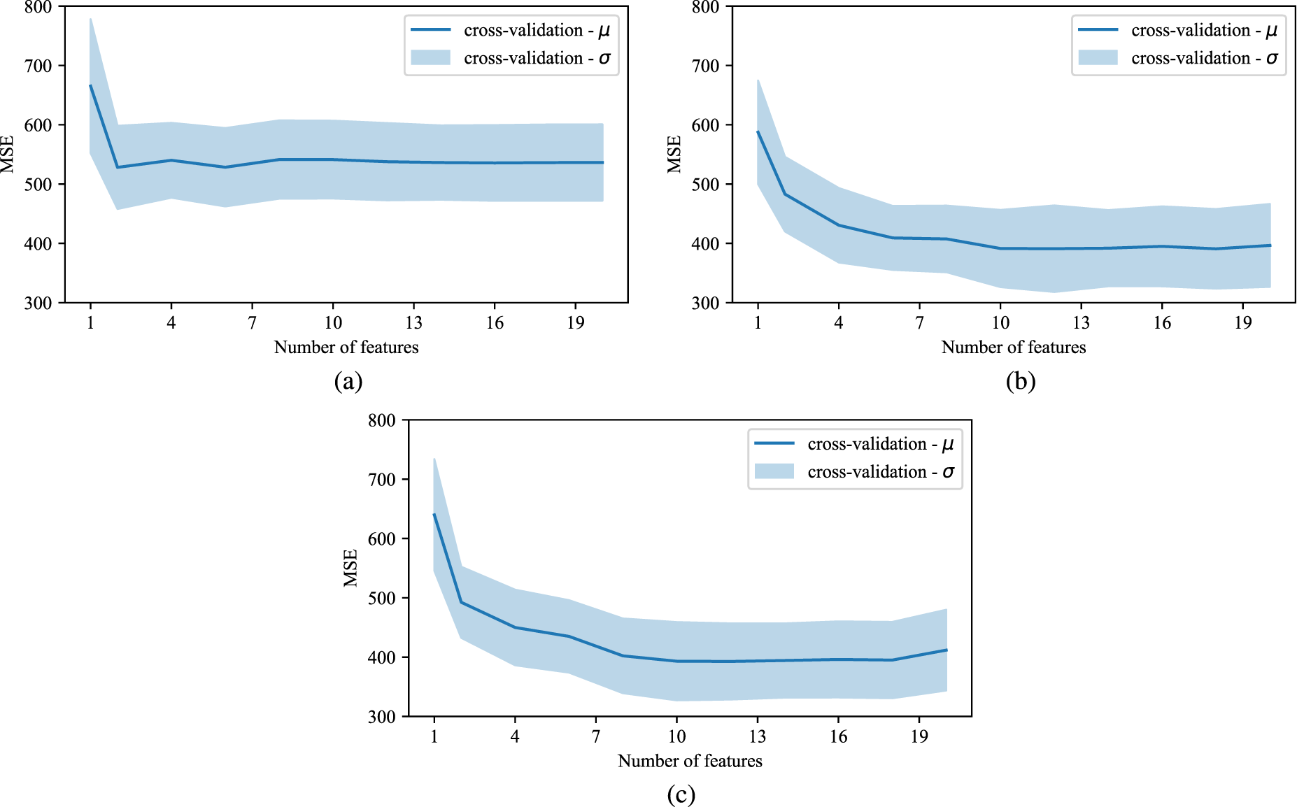
Cross-validation results of reverse-feature elimination with hyper-parameter tuning process: (a) linear regression; (b) gradient boosting; (c) random forest.
To estimate plan lead times, we need to derive a representative purchase order from historical purchase orders for each SKU. We pass the representative purchase order’s feature set into our trained machine learning model and use the response value as new plan lead times. The approach is rather trivial: To calculate a representative purchase based on information from the train-set, we take averages for the numerical values. For categorical values we take the most frequent value.
Prediction Accuracy
We analyze the accuracy of our models in predicting purchase order lead times for our test set. 490 SKUs were newly introduced, for which traditional forecasting techniques like SES can not be applied due to the absence of historical data. Figure 5 illustrates the prediction errors for different lead time forecasting methods. While the top graphs show the MSE, the graphs in the middle show the MAPE, and finally the bottom graphs show the bias. The metrics for the three graphs on the left were calculated for all 7,667 SKUs and the metrics for the graphs on the right were calculated for the subset of 7,177 SKUs for which historical data exists.
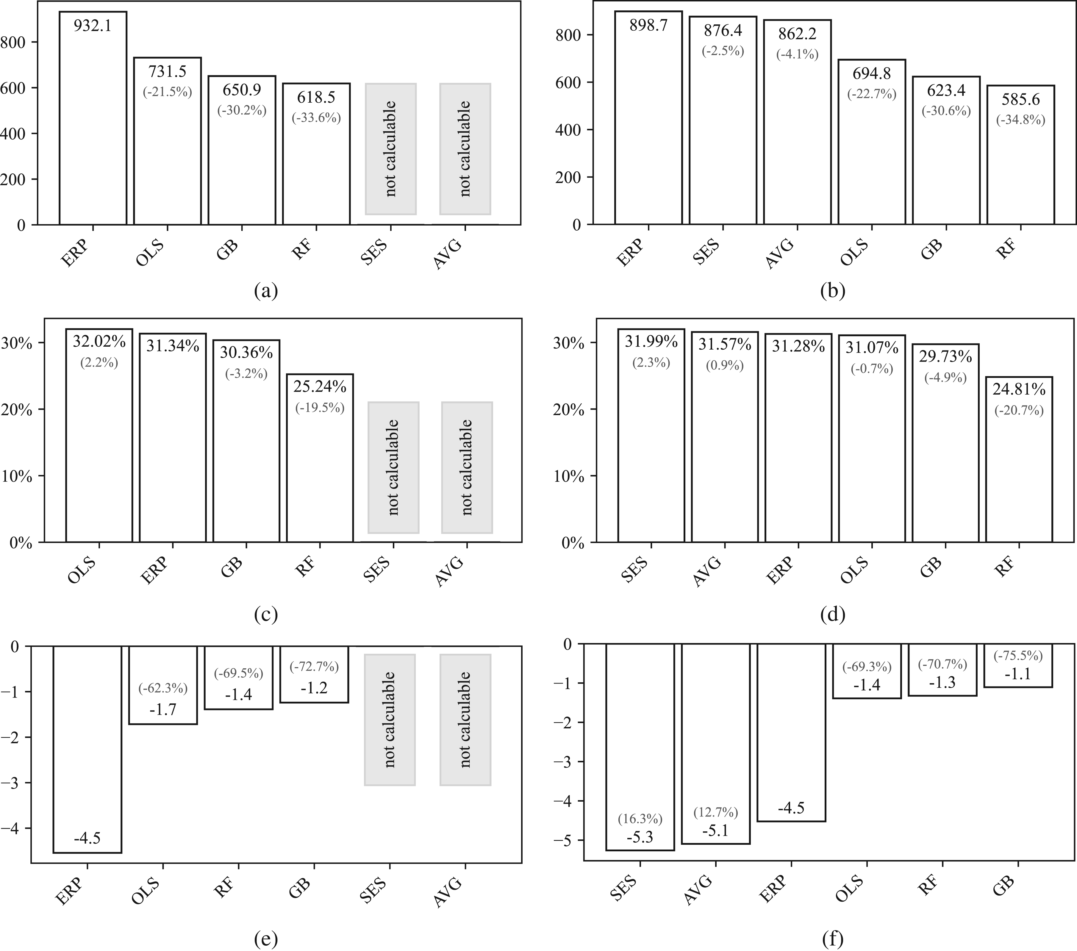
Accuracy of different potential plan lead times: (a) all SKUs
To analyze our numerical results, we first focus on MSE for SKUs with demand in the training set, as shown in Figure 5(b). The data indicates that algorithms, in general, provide more accurate lead time predictions than those from the ERP system. In bench-marking classical methods against regression methods, the latter demonstrate improved MSE outcomes compared to methods such as SES and historical averages. SES and historical averages perform similarly. The inclusion of additional features in regression models appears to contribute to their enhanced predictive performance. Within the category of regression models, it is the machine learning models, gradient boosting and random forest, that further enhance the predictive accuracy. Within this subset, random forest stands out, improving MSE by 34.84% over current ERP plan lead times, marking a significant improvement in forecast accuracy.
After confirming the effectiveness of the random forest model in terms of MSE for SKUs with demand in the training set, we examine the other graphs for consistent patterns. Upon extending the analysis to all SKUs as shown in Figure 5(a), consistency in algorithmic performance is observed even when evaluating SKUs without demand in the training set, with the random forest maintaining its lead in predictive accuracy. A similar improvement is observed in Figure 5(c) and (d). The random forest model not only lowers MSE but also reduces MAPE by 2.62 and 3.11 percentage points, respectively, which corresponds to improvements of 8.36% and 9.94%. These reductions underscore the model’s increased predictive accuracy, confirming that the improvements are not disproportionately affected by outliers.
Continuing the analysis, we observe that both historical averages and SES exhibit a notable negative bias, as shown in Figure5(f), aligning with expectations given the approximate 6-day shift in average lead times between the training and test sets (cf. Section 4.1). These methods inherently lack the capability to adapt to future developments. Consequently, their performance during inference is suboptimal. In contrast, current plan lead times (ERP) incorporate some level of foresight by reflecting temporal adjustments made by planners or adjustments derived from contractual obligations. This foresight allows for the anticipation of potential shifts. However, these plan lead times systematically underestimate actual lead times, as shown in Figure 5(e) and (f), indicating a persistent negative bias.
Regression models, particularly machine learning approaches like gradient boosting and random forest, are designed to identify and adjust for underlying data patterns. This capability enables them to effectively “debias” their predictions, as evidenced by the minimal bias observed even amidst slight shifts between training and test data. The high accuracy and low bias exhibited by these models demonstrate their robustness and their ability to generalize effectively to new data.
By evaluating model performance in relation to the order frequency in the training set, we gain insights into the reliability of our predictive methods for SKUs with varying levels of historical data. Figure 6 presents the performance of different forecasting methods against the procurement frequency of SKUs from the training set. The frequency categories range from “new,” indicating no historical procurement data in the train-set, to “monthly,” indicating frequent procurement. The graph plots the performance of our best performing machine learning model (random forest), current plan lead times (ERP), as well as conventional statistical methods (SES and historical averages). It illustrates a trend towards improved performance as the procurement frequency increases, signifying better accuracy with more data.
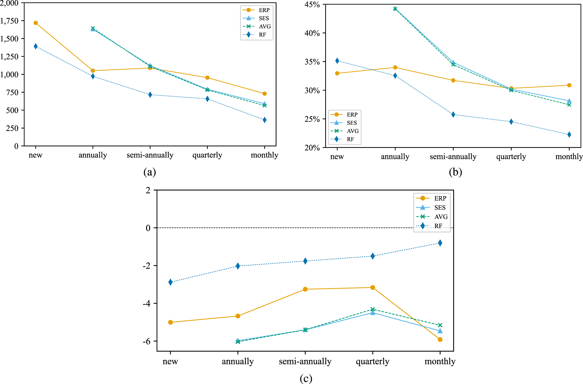
Accuracy of different potential plan lead times relative to order frequency: (a) MSE; (b) MAPE; (c) bias.
Notably, the random forest model consistently outperforms both the current plan lead times and classical statistical measures across all performance measures and almost all frequency categories. For instance, for new SKUs our method delivers an MSE roughly 25% lower than that of the current plan lead times. This significant reduction in error is indicative of the robustness of our method, particularly for SKUs without prior order history.
To generate some insights into how the features contribute to the prediction, we show the feature importance for random forest and gradient boosting in Figure 7. It becomes evident that the current plan lead time is a dominant feature, suggesting that the models heavily utilize this information to refine their predictions.
However, the significance of the “Long tail lead time,” “Cluster feature” and the advanced encoding of “Part ID” and “Supplier ID” emphasize the critical role of feature engineering in enhancing model performance. It indicates that the models are not solely reliant on current lead time parameters and historical lead times but also on the nuanced interplay of SKU characteristics. These features capture underlying patterns and similarities across SKUs that are otherwise not directly observable, thus providing powerful predictors that complement and enhance the historical data. Their substantial role in both models underscores the effectiveness of our feature engineering process, greatly enhancing the model’s ability to forecast lead times accurately.
In conclusion, the findings suggest that machine learning regression models, particularly the random forest, offer substantial improvements over traditional statistical methods and current ERP planning estimates in predicting lead times.
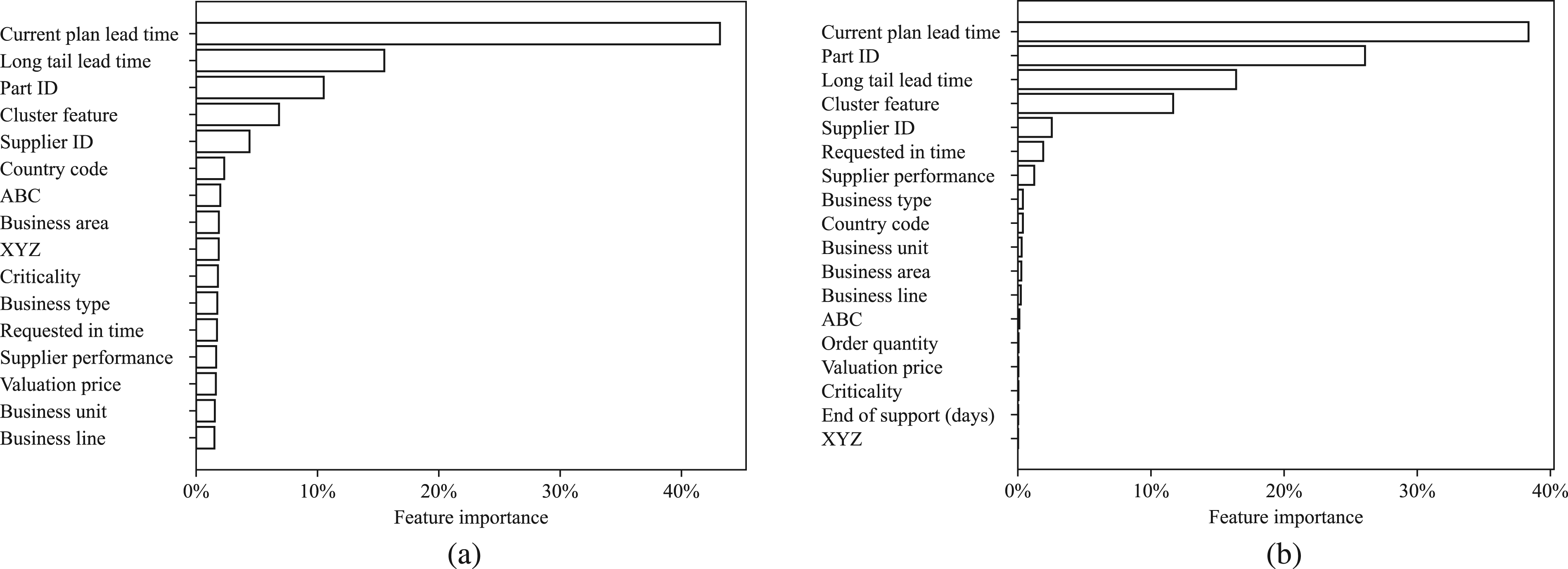
Feature importance: (a) random forest; (b) gradient boosting.
To quantify the expected business benefits of increased plan lead time accuracy we conduct a simulation study. We evaluate how the more accurate plan lead times also improve the company’s inventory performance. In our simulation, we compare how inventory levels evolve, using (a) the current plan lead times, and (b) the improved plan lead times. We use actual historical lead times for our benchmark. Our purchase orders hold information on when replenishment orders were submitted and when they arrived. We can simulate a realistic inventory development on an SKU level by modeling a periodic review base-stock policy with base-stock level S (Silver et al., 2016). This inventory control policy is applied in many real-world spare parts inventory systems (Boylan and Syntetos, 2010; Cavalieri et al., 2008; Syntetos et al., 2012; Wang, 2012) and also used by the company.
The intraperiod timing assumptions for the base-stock policy are as follows: each SKU is reviewed daily, and if the inventory position is below the base-stock level
To determine the appropriate base-stock level
Therefore, we use the lead time demand distribution to calculate the base-stock level
For fast-moving items, the assumption of normally distributed lead time demand is typically reasonable. However, our SKUs often exhibit intermittent demand patterns that the normal distribution may not represent. This is almost invariably the case for spare parts (Turrini and Meissner, 2019). For slow-moving items the poisson distribution typically offers a good fit for the arrival of spare part demand (Silver et al., 1998). For demands that are not unit-sized but of constant size the resulting distribution of demand per period can be modeled by a “package Poisson” distribution (Ritchie and Kingsman, 1985). If demand size is not constant, it is reasonable to assume that demand arrivals are poisson distributed, and the order size follows a logarithmic distribution. In such cases, total demand is negative binomial distributed over lead time (Quenouille, 1949). For our simulation, we use negative binomial distributions to model our spare part demand, noting that the Poisson distribution is a special case of this distribution.
To compute the moments of the distributions, it is necessary to forecast both lead time and demand. We utilize the predicted lead times to estimate the average lead time, denoted as
The moments of the lead time demand distribution are calculated using established formulas for the mean and variance of the sum of a random number of random variables
To determine the appropriate base-stock level, we aim to ensure that the expected back-orders during a replenishment cycle do not exceed a specified fraction of demand within the same cycle. This objective is formalized through the following optimization problem (Sieke et al., 2012):
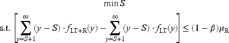
We use
For our simulation, the initial inventory position starts at the respective base-stock level
The amount of capital lockup has been scaled linearly in order to not reveal information about the company. Figure 8 summarizes our simulation results. The trade-off curve shows the capital lockup for a given realized service level. The grey curve shows inventory performance based on base-stock levels
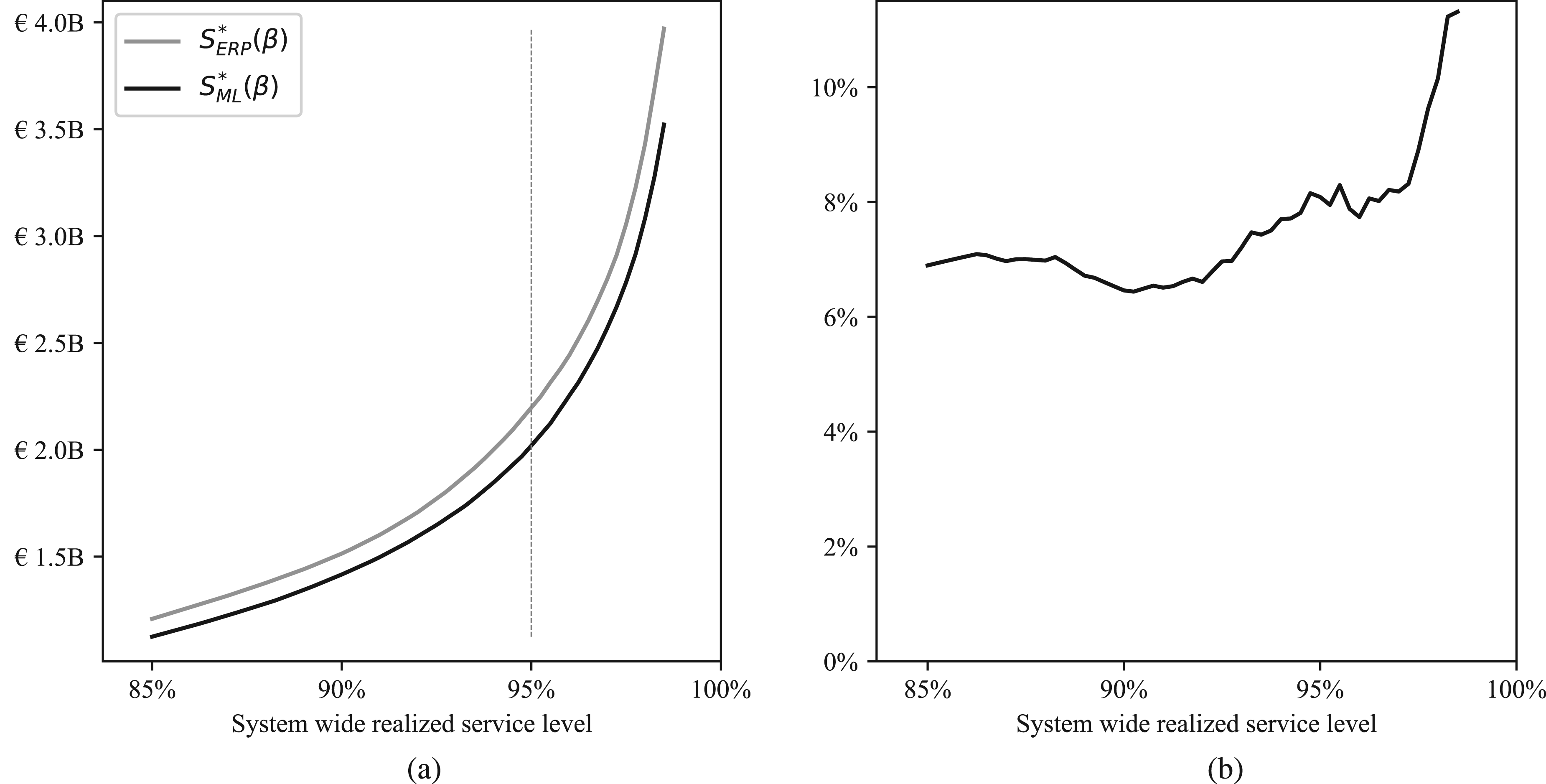
Simulation results: (a) capital lockup for a given realized service level; (b) capital savings (%) for a given realized service level.
The black curve is constantly below the grey curve, implying that compared to the current plan lean times, our approach leads to stock levels that achieve higher service levels while having the same capital lockup. To derive some financial implications of our proposed method, we investigate inventory performance for an achieved 95% service level. We find that to attain the targeted service level, base-stock levels
Implications
The implications that we derive from our results provide recommendations for implementing lead time prediction approaches with machine learning and how they can be used in practice to exploit potential benefits.
Effective feature engineering can provide significant benefits. In our spare parts setting, data on SKU level is often limited. We successfully develop a text classification algorithm to incorporate information from similar SKUs based on their descriptions. Additionally, we enrich our data set with general information on supplier performance. State-of-the-art algorithms allow us to train our models on sparse categorical features. While conducting our study, we have found that there is a relationship between the extent of information extraction from the available data and the accuracy of our models. The feature importance analysis in Section 4.2 has clearly indicated that the additional features derived from feature engineering significantly contribute to accuracy improvements for all machine learning models we investigate.
Machine learning enables a more accurate prediction of lead time solely based on observed purchase orders. There are very few studies attempting to predict lead times solely based on the limited information available at a company. Companies often depend on (a) lead times specified in supply contracts, (b) employees’ experience, or (c) average values based on historical data. We have seen that (a) lead times specified in supply contracts can significantly deviate from actual lead times. (b) Relying on expert knowledge can result in predictions being biased by stock-out aversion. Additionally, by relying on human experience, the company is exposed to the risk of unique human knowledge leaving the company in employee churn. (c) Average values based on historical data have been shown to be limited by the frequency of observations.
Our results align well with current evidence from an emerging stream of literature addressing the viability of machine learning applications for lead time prediction. We contribute to this literature stream by confirming that machine learning applications can reliably predict lead times with high accuracy. This is an opportunity for many companies to predict lead times operationally and take short-term measures. Indications as to whether an order arrives earlier or later than expected can be used to manage critical inventories tightly.
Plan lead times derived from machine learning are particularly valuable for procurement structures with large number of different SKUs with only a few purchase orders each. We have shown that compared to other alternatives, our method performs best for SKUs that are more frequently procured than once every half a year. This demonstrates a major advantage of our machine learning approach to determine plan lead times compared to methods that rely solely on past data: the data for available SKUs can be exploited to predict lead times for SKUs with an insufficiently large set of historical data. With increasing procurement frequency the accuracy of other methods converge, due to many observations being available from which estimates can be derived.
Plan lead time accuracy improves inventory performance. When lead time is used in the planning process to set inventory control parameters, increased lead time accuracy is expected to improve business outcomes. The business benefits of increased plan lead time accuracy are challenging to quantify since they are based on adjusted processes to reflect the improved accuracy. Therefore, we simulated inventory developments based on current and improved plan lead times. We estimate that for achieving a targeted service level of 95%, our approach is expected to reduce capital lockup by 7%.
While the findings in our study are promising, it is important to discuss the generalizability of these results. Our primary goal is not to identify a universally superior model but to demonstrate the benefits of applying machine learning techniques to lead time prediction in contexts characterized by sparse data and lead time uncertainty, such as spare parts management. A distinct and important contribution of our paper, compared to the existing literature, is our focus on predicting the lead time distribution from the supplier’s perspective. Suppliers, who order from various manufacturers, often have limited information about the production state of products and manage a wide variety of product types. Our methodology addresses this complexity by using machine learning to effectively handle diverse and incomplete data, enabling more accurate predictions of lead times.
The higher accuracy of the random forest model in our study can be attributed to its robustness against skewed feature distributions and its ability to handle complex, non-linear relationships. However, we recognize that these findings may not directly apply to all contexts. Supply chain environments vary significantly, with differences in data availability, supplier behavior, and SKU characteristics. Consequently, no single model is likely to consistently outperform others across all scenarios. Therefore, while random forest demonstrates high effectiveness in our setting, we do not claim it will always be the best-performing model.
Our findings emphasize the critical importance of robust feature engineering and the incorporation of domain-specific knowledge. These elements are likely to be more decisive in the success of any machine learning model for lead time prediction than the specific choice of algorithm. The general methodology we use is likely to yield good results in similar contexts where suppliers face uncertainty due to diverse products and limited visibility into production processes. This adaptability underscores the broader applicability of our approach beyond our specific study.
Our study offers a scalable and solid methodology that can be adapted by researchers and practitioners alike to address the challenge of lead time prediction in various contexts, particularly those involving spare parts with limited historical data. As more companies develop in-house data science capabilities, implementing these advanced techniques becomes increasingly feasible and less resource-intensive. Although implementing data collection processes and operationalizing machine learning pipelines may initially seem complex and costly compared to simpler methods like SES, the significant accuracy improvements demonstrated in this study make a strong case for the investment.
We have successfully implemented this machine learning tool within a company, demonstrating its practical applicability and tangible benefits. The long-term cost savings from more accurate lead time predictions, as evidenced by our simulation, are likely to outweigh the initial implementation costs. The strategic advantage gained through improved inventory management and procurement processes justifies the complexity of the machine learning methods used. This approach provides a robust framework for companies to enhance operational efficiency and make informed decisions, thereby transforming how lead time predictions are handled in practice.
Limitations
In this study, we derived accurate plan lead times for SKUs. These plan lead times are point estimates of lead time which are used by optimization tools for inventory planning to set inventory control parameters. While many firms use inventory management software ignoring lead time uncertainty (Dolgui et al., 2013), lead time fluctuations strongly degrade the tools’ performance and cause high inventory costs. Babai et al. (2022); Chopra et al. (2004); Song et al. (2010), as well as others, have demonstrated the economic implications of lead time uncertainty. They have shown the importance of accounting for its effects regardless of the procedures used to compensate for demand uncertainty.
In addition to our proposed machine learning approach, it is important to acknowledge that alternative or complementary strategies, such as continuous improvement methodologies, could be employed to improve plan lead time accuracy. Continuous improvement could involve identifying and focusing on the most critical or problematic parts and suppliers to either better predict lead times or create robust processes that can respond to the uncertainty. By integrating such continuous improvement efforts with machine learning models, companies can potentially enhance their overall planning accuracy and operational resilience.
In this study, we also illustrate the impact that ill-estimated lead times can have on inventory performance. Yet, we only cover the forecasting of point estimates of lead time. Modern optimization tools account for lead time uncertainty and depend on estimates on the lead time uncertainty, that is, the variance of the response value (Cachon and Terwiesch, 2008; Silver et al., 2016; Song et al., 2010).
In the future it would be great if the methods we describe in our article, were used for non-parametric conditional density estimation (Bertsimas and Kallus, 2020; Dalmasso et al., 2020; Pospisil and Lee, 2018). The conditional density estimation could be used to estimate lead time demand directly fitting into recent research of Babai et al. (2022); Boylan and Babai (2022). Their research is dedicated to estimating lead time demand distributions directly, albeit considering only univariate lead time samples.
Conclusion
In this study, we addressed the challenge of maintaining inaccurate master data on which many inventory optimization models rely. We investigated with special regard to plan lead times how well the maintenance of this planning parameter can be automated by means of machine learning.
We applied unsupervised and supervised machine learning in our lead time prediction approach. Based on natural language processing techniques, we identified similar SKUs and used this information to generate features for our model. To derive plan lead times from our machine learning models, we used the features of representative purchase orders to generate a response value from our model. This value can be used as plan lead time.
We tested our approach on historical data of a global equipment manufacturer. We bench-marked the results against current plan lead times from the company as well as simple statistical measures of central tendency. We found that our approach significantly increases the accuracy of plan lead times by over 30% compared to current plan lead times. Simulations have shown that the increased accuracy of plan lead times reduces capital lockup by approximately 10% while increasing the likelihood of achieving the targeted service level for a given capital lockup. This translates into significant cost reduction for inventory-keeping as well as into reputational benefits due to fewer back-orders. Moreover, we developed a method to predict lead times for new SKUs, which can be used as decision support for contract negotiations with the suppliers. With specific regard to plan lead times, machine learning has proven to be a viable technique for improving the quality of master data. Thus our method creates tangible and intangible added value by automating a notoriously tedious and error-prone task.
Footnotes
Acknowledgments
The authors are grateful to the editors and the anonymous review team for the insightful guidance provided throughout the revision process. The authors would also like to thank all research participants and organizations involved in this research study for their support.
Declaration of Conflicting Interests
The authors declared no potential conflicts of interest with respect to the research, authorship, and/or publication of this article.
Funding
The authors received no financial support for the research, authorship and/or publication of this article.
How to cite this article
Reiners R, Haubitz CB and Thonemann UW (2025) Lead Time Prediction for Inventory Optimization With Machine Learning. Production and Operations Management 34(10): 3010–3025.