
Abstract
Reverse factoring (RF) is a highly relevant form of supply chain finance. Whereas extant analytical studies indicate how RF should enable buyers to extend payment terms, sufficient empirical evidence is lacking. To hypothesize on payment term extensions, we study three motives—financing cost, fairness, and standardization. Our empirical evidence indicates the presence of all three. It extends former analytical work on RF adoption revolving around the financing cost motive only.
Introduction
Even buying firms with solid credit ratings turn to their supply chain to reduce their financing costs and improve their working capital (Filbeck et al., 2017). They pay their suppliers according to long payment terms (Hu et al., 2018), such as when Boeing increased its payment terms to 120 days, as opposed to 30 days (Scott and Hepher, 2016), and Anheuser Busch InBev strived for payment terms of 120 days (Daneshkhu and Shubber, 2015). Procter & Gamble demanded its suppliers to wait 75 days until getting paid, resulting in increases of about $1 billion in its cash flows (Strom, 2015). Suppliers in weaker bargaining positions often feel more compelled to accept the longest payment terms, whereas more powerful suppliers get paid faster (Fabbri and Klapper, 2016). However, putting financial pressure on weaker suppliers increases their economic risk (Boissay and Gropp, 2007).
To extend payment terms with all suppliers without jeopardizing the liquidity of the upstream supply chain, many large buying firms have adopted reverse factoring (RF) (Herath, 2015; van der Vliet et al., 2015; Wuttke et al., 2019). With a potential market volume of $20 billion (Herath, 2015) and a quickly growing number of significant firms using RF (e.g., Walmart 1 and Michelin 2 ), RF is among the most important supply chain finance arrangements. RF always involves a buying firm, a supplier, and an RF provider (which may be a bank). After the buying firm’s invoice approval, the RF provider immediately pays suppliers in the RF program. The suppliers receive the total invoice amount minus an RF interest charge. This charge depends on the payment term (the longer the payment term, the higher the cost), as well as on the buying firm’s usually strong credit rating, such that it tends to be cheaper for the suppliers compared to other sources of financing (otherwise, they typically would not use RF). At the end of the payment term, the buying firm pays the RF provider the total invoice amount. Suppliers thus benefit from reduced financing costs, paying their buyer’s interest rate instead of their own. So, buyers can use RF to extend payment terms without sacrificing their upstream supply chain’s liquidity. However, the question arises: How much can they extend payment terms for each supplier? Would it be worth the effort required to adopt RF?
To predict payment term extensions, buyers must likely account for more than the interest rate difference. Discussions with and publications by RF providers indicate some potentially relevant motives. CRX Markets and Citibank, for instance, emphasize financing costs by offering online calculators. 3 With their online tools, managers can enter the current conditions (payment terms and interest rates) and the RF conditions (new payment terms and RF interest rate) and calculate the supplier’s savings. This helps to indicate the considerable potential to extend payment terms. In addition, PrimeRevenue mentions fairness concerns, 4 picking up on the criticism that RF helps powerful buyers to extend payment terms unduly (Pettypiece et al., 2015). This fintech emphasizes that managers also consider whether they perceive an agreement as fair. Or consider Orbian, whose chairman recently emphasized the potential of standardizing payment terms with RF. 5 Buyers that standardize payment terms reduce the differentiation among their suppliers, they can reduce the administrative effort required for managing different terms, and reduce errors resulting from a lack of standardization. Do all three motives—financing cost, fairness, and standardization—affect payment term extensions? Or is the financing cost motive the sole driver in industry? After all, the primary motivation for adopting RF is to extend payment terms (Liebl et al., 2016; Wuttke et al., 2013). In addition, the financing cost motive is most central to extant analytical studies on RF (Hu et al., 2018; Kouvelis and Xu, 2021; Lekkakos and Serrano, 2016; Tanrisever et al., 2012; van der Vliet et al., 2015; Wuttke et al., 2016). In contrast, neither fairness nor standardization motives have received the same academic attention in the context of RF adoption (with the exception Banerjee et al., 2021). Put differently, how much should managers rely on RF providers’ statements on fairness and standardization? Do they play a role?
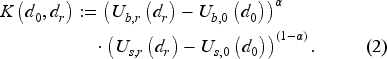
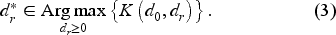
To provide answers, we derive a Nash bargaining model with financing cost, fairness, and standardization motives. Building on our analytical results, we derive hypotheses and test those on a dataset of
Related Literature
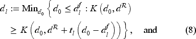
The finance and operations interface is receiving increasing attention (Babich and Sobel, 2004; Kouvelis and Zhao, 2012; Zhao and Huchzermeier, 2015). Many studies indicate that cash flow optimization and liquidity management are important objectives complementing profit maximization (Boissay and Gropp, 2013; Filbeck et al., 2017; Kouvelis and Zhao, 2012). Empirical studies find how firms agree on payment terms without RF (Fabbri and Klapper, 2016; Summers and Wilson, 2002). Powerful buyers often bargain for long payment terms (Fabbri and Klapper, 2016). By enabling faster cash flows, RF directly affects this decision.
There are several empirical, operations-management-related studies on RF. Liebl et al. (2016) and Wuttke et al. (2013) both derive insights using case studies. Liebl et al. (2016) explores the objectives of, antecedents to, and barriers to RF adoption. They find that buyers mainly adopt RF to extend payment terms and reduce supply chain risks. Wuttke et al. (2013) focus on the adoption process from a buying firm’s perspective and find that RF adoption requires a series of organizational and procedural adjustments. Wuttke et al. (2019), studying the adoption of RF by suppliers, derive and test efficiency and legitimacy motives as drivers. They find that suppliers adopt RF faster if they are small, expect big benefits, and face considerable institutional pressures. However, to the best of our knowledge, no empirical study examines how buyers extend payment terms, and when they extend by more or fewer days.
Prior analytical studies typically depart from inventory models (Kouvelis and Xu, 2021; Lekkakos and Serrano, 2016; Tanrisever et al., 2012; van der Vliet et al., 2015), models of financial flexibility (Grueter and Wuttke, 2017; Hu et al., 2018), or innovation diffusion models (Dello Iacono et al., 2015; Wuttke et al., 2016) in their effort to identify the RF value proposition. Those studies typically characterize the optimal payment term extensions, noting that, in equilibrium, those tend to be positive (Hu et al., 2018; Lekkakos and Serrano, 2016). The objective of virtually all game theoretic models of RF is to understand underlying tradeoffs and mechanisms (Grueter and Wuttke, 2017; Hu et al., 2018; Kouvelis and Xu, 2021; Lekkakos and Serrano, 2016; Tanrisever et al., 2012; van der Vliet et al., 2015; Wuttke et al., 2016). Whereas they all provide fascinating insights and often counter-intuitive results, their purpose is not necessarily to explain actual behavior. So, despite their mathematical rigor, it might be that the empirical setting differs from some assumptions, limiting the scope for predictions. We complement this literature as we provide a parsimonious model seeking to describe actual behavior so that we can test our predictions with data from RF programs.
Whereas most studies on RF examine financial aspects, Banerjee et al. (2021) examine RF adoption decisions through a choice-based conjoint experimental design. In their experiment, subjects refused RF adoption significantly more often when they perceived unfairness. We also consider fairness but study its effect on a bargaining outcome instead of the adoption decision. We further examine actual decisions in a secondary-data study. More generally, we draw from the literature on fairness concerns in economics. Fairness concerns can have strong implications (Thaler, 1988). Hoffman et al. (1996) demonstrates that decision-makers care for fairness even when stakes are high. A result that Fehr et al. (2002) later confirmed. The theory on fairness is broad and features many fairness aspects (see Fehr and Schmidt, 1999). An important observation is that fairness concerns do not necessarily result in equal profit splits. Still, they foster bargaining outcomes that both parties deem more appropriate. We relate primarily to those studies that examine how fairness concerns affect decisions in supply chains like Cui et al. (2007), providing a game-theoretical model of fair-minded supply chain firms, and Cappelen et al. (2007), examining various fairness ideals in experiments. In our model, we also assume actors to be fair-minded as we model the case where neither firm wants to end up below their fairness ideal.
Finally, Osadchiy et al. (2024) relates to the standardization of payment terms. Those authors study customer portfolio approaches to managing cash flow variability. They demonstrate empirically that suppliers selectively offer standardized payment terms to new customers. Their study indicates suppliers benefit from standardizing payment terms among their buyers.
Analytical Predictions
We derive analytical predictions on payment term extensions, complementing extant RF research in three regards. First, we learned from RF professionals that buyers rarely make final take-it-or-leave-it offers like Stackelberg leaders. This intuitive observation is consistent with empirical studies examining how firms agree on payment terms (Fabbri and Klapper, 2016; Summers and Wilson, 2002). Therefore, we assume Nash bargaining instead of a Stackelberg game.
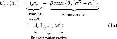
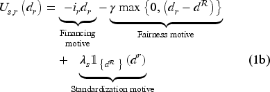
Second, we learned from those professionals that negotiators often refer to (un-)fairness, such as when buyers argue that short payment terms are unfair or suppliers complain about unfair long payment terms. Such a reference to fairness can help to shape negotiation outcomes (Voss and Raz, 2016). Fairness concerns are established in the economics literature (e.g., Fehr et al., 2002; Hoffman et al., 1996). Consistent with our discussions and those studies, we introduce the notion of fairness concerns (Banerjee et al., 2021; Cappelen et al., 2007; Cui et al., 2007) to bargaining over payment terms in the RF context. Buyers (suppliers) perceive disutility if their new payment terms fall below (exceed) a reference point, such as typical payment terms (e.g., 90 days). Therefore, it is not the extension per se that is deemed fair or unfair but the comparison of new payment terms and the reference point.
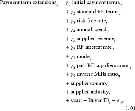
Third, we introduce standardization benefits, which professionals likewise mentioned. Those benefits arise when payment terms become identical among multiple firms, reducing differentiation, the administrative effort required for managing contracts, and the risks of errors. Standardized customer payment terms can further reduce cash flow volatility (Osadchiy et al., 2024). Therefore, we assume that buyers (suppliers) benefit when RF leads to standard payment terms among their suppliers (buyers).
Model
The status quo is the best alternative to a negotiated agreement. Consider buyer
Both players bargain over the RF payment terms,
To avoid extreme cases, we assume a reasonable reference point with
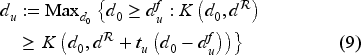
To study the effect of the fairness and standardization motives more explicitly, we first provide a hyper-rational benchmark where actors only care about the financing cost motive. Please find all proofs in the e-companion.
Hyper-rational benchmark
Suppose

If only the financing cost motive is present, payment terms under RF thus linearly increase in initial payment terms,
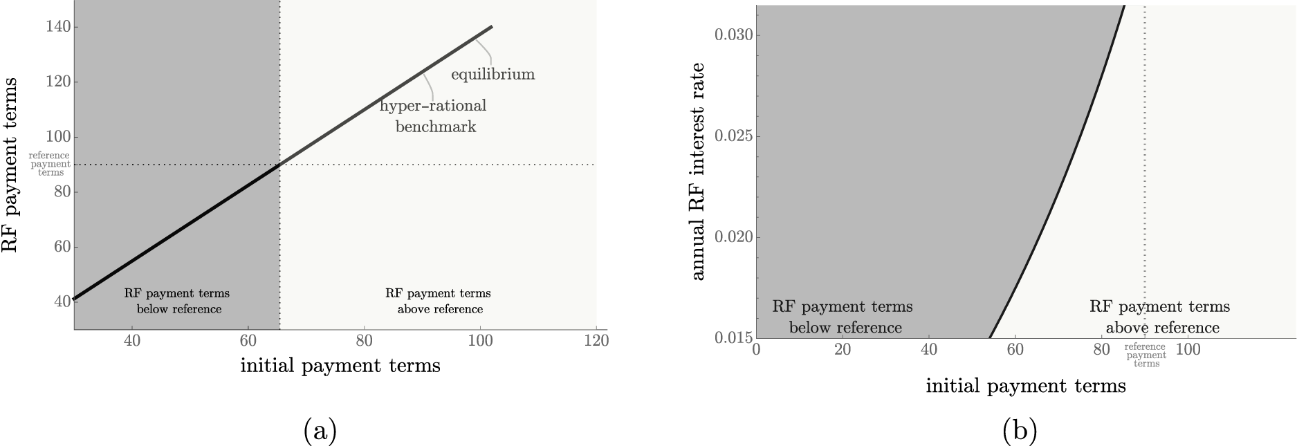
Financing cost motive (hyper-rational decision makers). (a) Reverse factoring (RF) payment terms. (b) RF equilibria.
Let us next turn to full model equilibrium with all three motives present.
(Full model)
Let

To explain the effect of the fairness and standardization motives on the bargaining outcome in this theorem, let us first consider the effect of the fairness motive while ignoring the standardization motive. Therefore, suppose

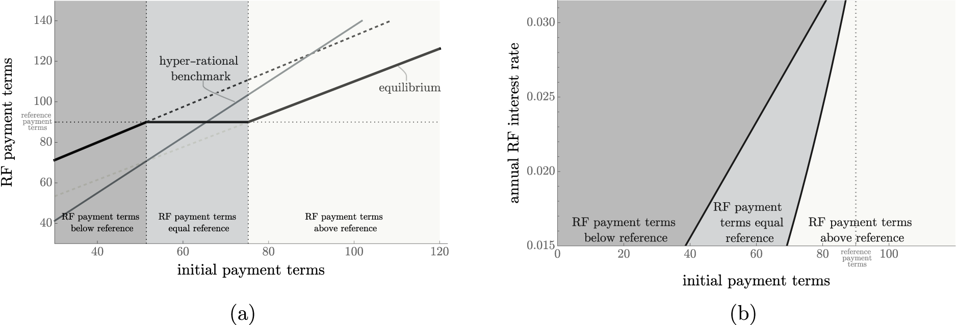
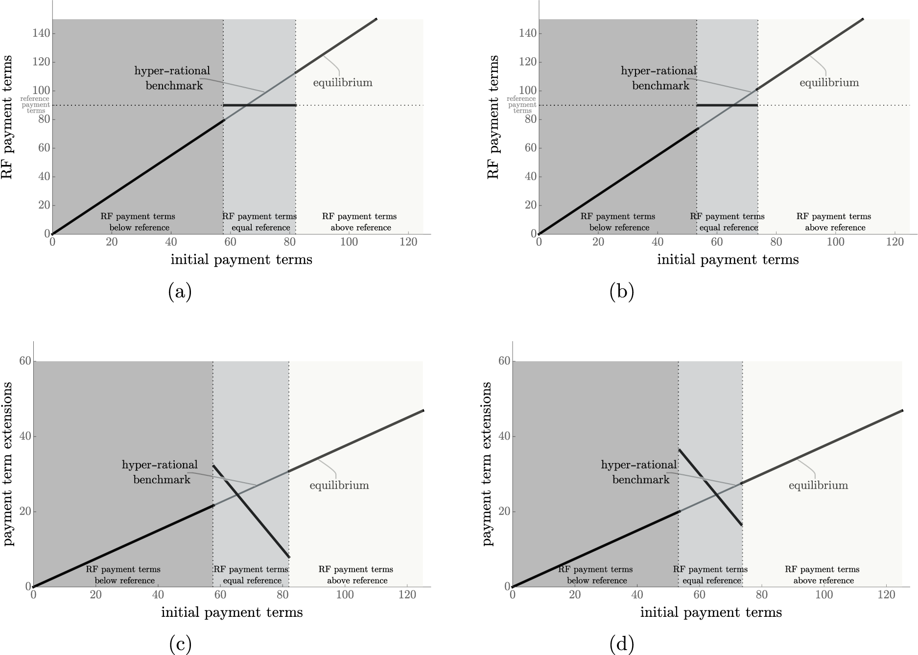
The fairness motive can lead to standardized payment terms. (a) Reverse factoring (RF) payment terms. (b) RF equilibria.
In Figure 2(a), the reference point, 90 days, is the outcome for all initial payment terms ranging from about 51 to 75 days, a range that depends on the RF interest rate (Figure 2(b)). Figure 2(a) further illustrates that, compared to the hyper-rational benchmark, the fairness motive can lead to larger RF payment terms (for
Defining payment term extensions as
Fairness motive. (a) No fairness motives (
Similarly, in Theorem 1, we can assume
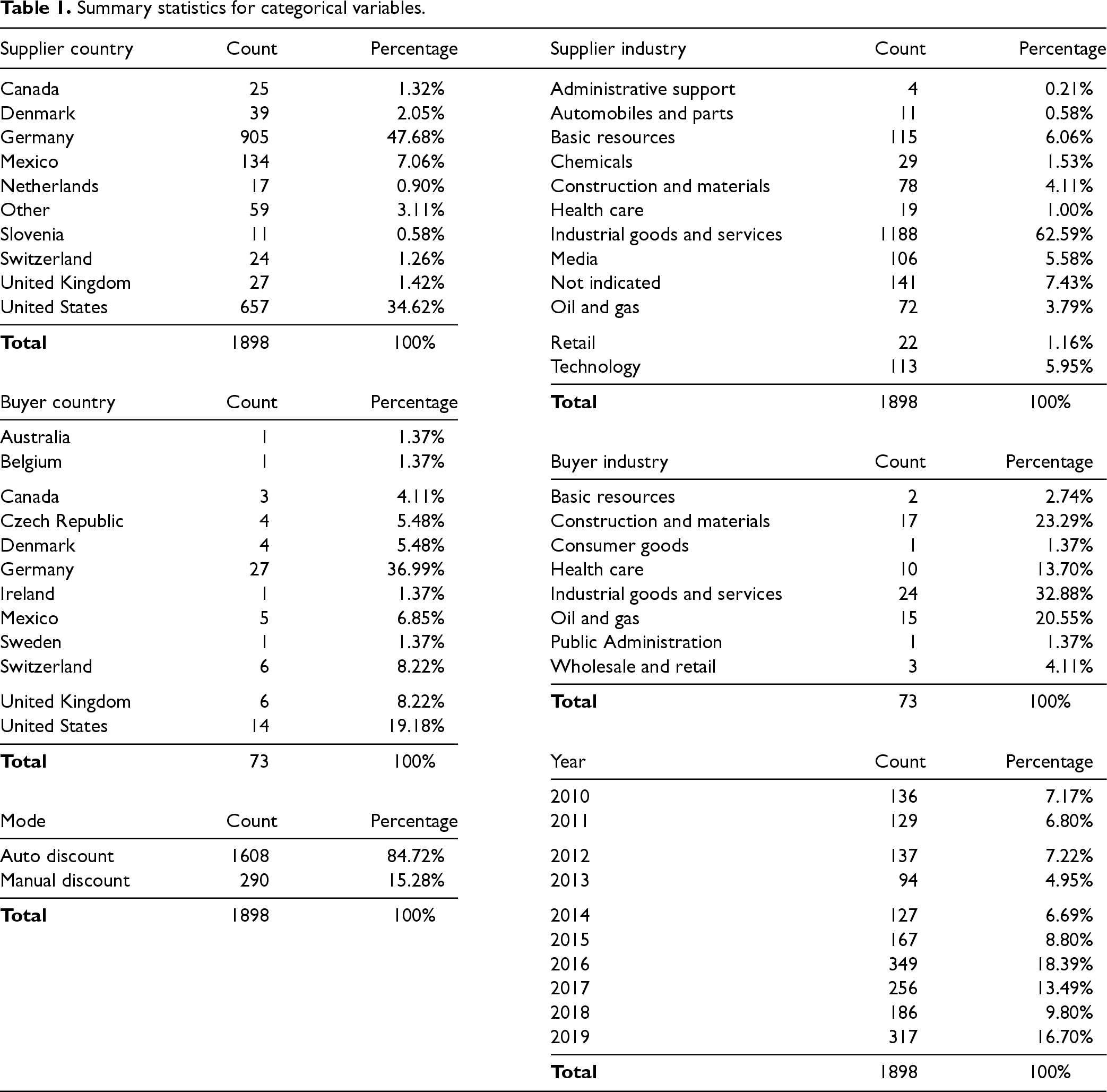
Standardization motive. (a) Reverse factoring (RF) payment terms (
We will present two corollaries on Theorem 1, which lead to testable hypotheses. We complement those with an hypothesis motivated by Theorem 1.
Initial payment terms will be extended due to RF unless they are in a specific interval. The extension is intuitive; after all, it is the buyer’s main intention when adopting RF. The buyer can benefit from standardization and accept shorter payment terms. However, this can happen only if the payment terms are just above the reference,
Hypothesis 1. The adoption of RF is associated with an extension of payment terms.
The next result examines the relationship between initial payment terms,
Suppose Suppose Suppose
Case (i) describes outcomes for relatively small initial payment terms (
Taken together, if
Hypothesis 2a. Longer initial payment terms are associated with longer extensions of payment terms under RF.
Conversely, if
Hypothesis 2b. Longer initial payment terms are associated with shorter extensions of payment terms under RF.
Theorem 1 in conjunction with Figure 4 predicts both a potentially positive and negative effect of standardization on payment term extensions. There are, however, some aspects that might favor a negative effect more. Buyers introduce an RF platform and can negotiate new payment terms with many suppliers. For them, striving for standardization can have strong effects. For instance, a buyer might be able to standardize payment terms for up to all suppliers. In contrast, the importance of standardization may be smaller for suppliers. They can only move terms to a new standard with one customer unless they are joining RF programs of other providers and other buyers. Therefore, we expect standardization benefits to be more important for buyers. When buyers benefit more from standardizing, we expect them to make stronger concessions regarding the extension of payment terms, resulting in
Hypothesis 3. Payment term standardization is negatively associated with payment term extension.
Our primary data source is a leading U.S.-based RF provider managing programs with large buyers. Each program includes multiple suppliers, but each supplier appears in only one program. This 1:n structure reflects buyers initiating RF programs and onboarding their suppliers. Buyers are geographically and industrially diverse, and suppliers, often small or medium-sized, do not overlap across programs. The RF provider charges no setup, operating, or consulting fees; instead, it embeds fees in the RF interest rate. Buyers and suppliers determine payment terms; the RF provider does not request specific terms. RF programs are long-term; no active supplier in our sample has left, with the earliest dyad lasting about ten years.
RF requires buyers to disclose a series of essential variables, such as buyer industry, buyer revenue, and buyer costs of goods sold. About 75% of the suppliers are private firms with no publicly available data; for RF, they do not need to inform the RF provider with the same level of details. Nevertheless, some supplier-level variables are still available in this dataset because each RF program features an RF platform. Buying firms can enter variables such as the initial payment terms and RF payment terms, as well as supplier industry, country, and revenue. The initial payment terms refer to the latest payment terms before adopting RF; the RF payment terms refer to the payment terms both parties agreed on when introducing RF. Buyers do not record the supplier’s interest rate outside RF. As we learned from the RF provider, suppliers are unwilling to disclose this information due to their concern that buyers or providers might use this sensitive information to their disadvantage in the long run. Few suppliers have a publicly documented credit rating, so the RF provider does not collect this variable.
The data refer to a period from 2010 to 2019, with 73 buyers and 1,898 buyer–supplier dyads with complete data. As the data collection ended in December 2019, none of the effects in our study were affected by the coronavirus disease 2019 (COVID-19) pandemic. All variables on the supplier level are recorded when the supplier adopts RF. All variables on the buyer level are time-invariant and capture the most recent date (December 2019). We used an earlier version of this dataset to investigate different research questions and hypotheses (Wuttke et al., 2019). In that former study, we investigated the speed at which suppliers adopt RF. In contrast, in this study, payment term extension is the dependent variable. The former research draws from theory on technology adoption, whereas this present study tests analytical predictions. For consistency, we followed the exclusion criteria of Wuttke et al. (2019) and removed extreme outliers (three interquartile ranges below (above) the first (third) quartile). The data still differs slightly since we use a more recent dataset. As one robustness check and for consistency, we examine our main model using the exact same dataset as in Wuttke et al. (2019).
When buyers and suppliers negotiate RF payment terms, they usually agree, and suppliers adopt RF. However, our dataset also encompasses data on 96 additional suppliers who ultimately decided against adopting RF. We include those 96 cases when estimating selection models.
We complemented this dataset with publicly available data. We used the London Interbank Offered Rate (LIBOR), a widely accepted reference rate for the short-term interest rate, to measure the risk-free rate. We use LIBOR data from the Federal Reserve Bank (St. Louis). The RF provider shared anonymous data without firm names for confidentiality reasons, which prevented us from collecting any further firm-level data.
Variables
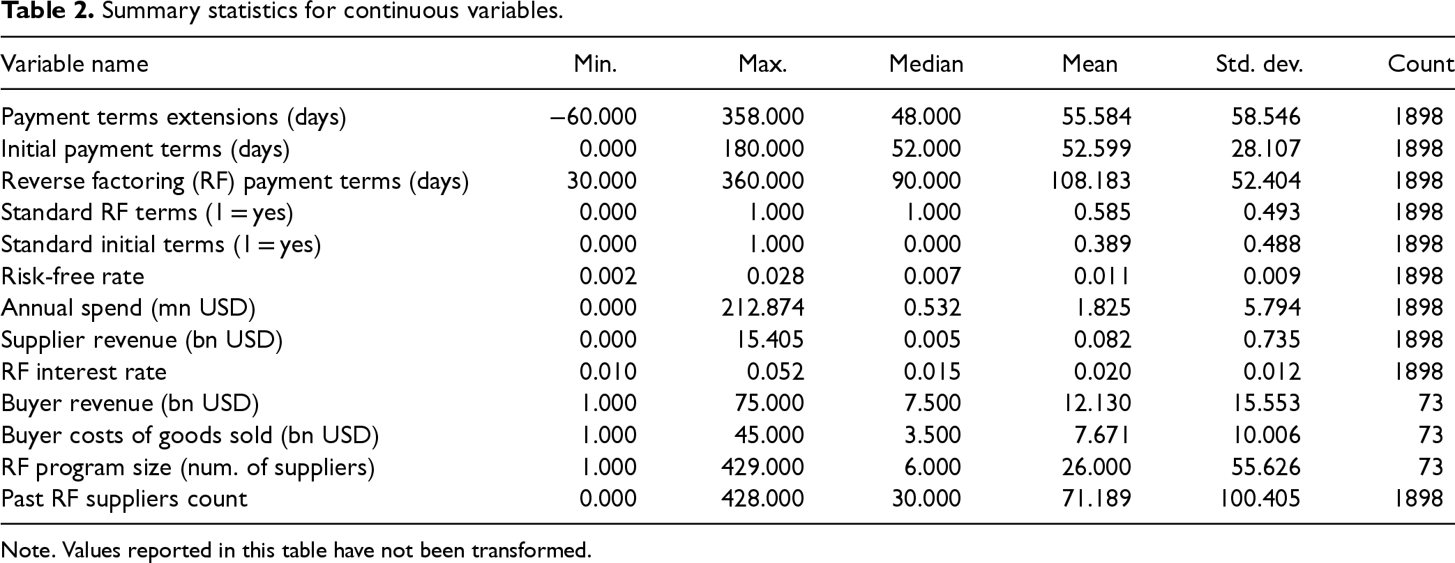
Table 1 provides an overview of the demographic variables of the suppliers that adopted RF (Table A1 in the appendix summarizes suppliers that did not adopt RF, suggesting no substantial differences). To obtain fairly balanced categories for supplier country and supplier industry, we decided to pool countries with less than ten suppliers into the category ‘other countries’; this category captures mostly small EU countries such as Belgium, Sweden, and Latvia. Table 1 also displays buyer country and buyer industry. These buyer-level demographic variables do not affect our primary analysis, so creating more balanced groups is unnecessary.
Summary statistics for categorical variables.
Summary statistics for categorical variables.
Suppliers can decide between two modes: Automatic or manual. Automatic refers to suppliers using RF for each invoice when the buyer approves it. Manual means that suppliers are informed whenever a buyer approves an invoice and then decide whether and when to use RF to convert the receivables into liquidity. By postponing this conversion, suppliers reduce the financing costs linearly. The factor variable mode is zero if the supplier uses RF automatically and one if it uses RF manually. About 85% of the suppliers in our sample use the automatic mode. The factor variable year captures when a supplier agrees to adopt RF.
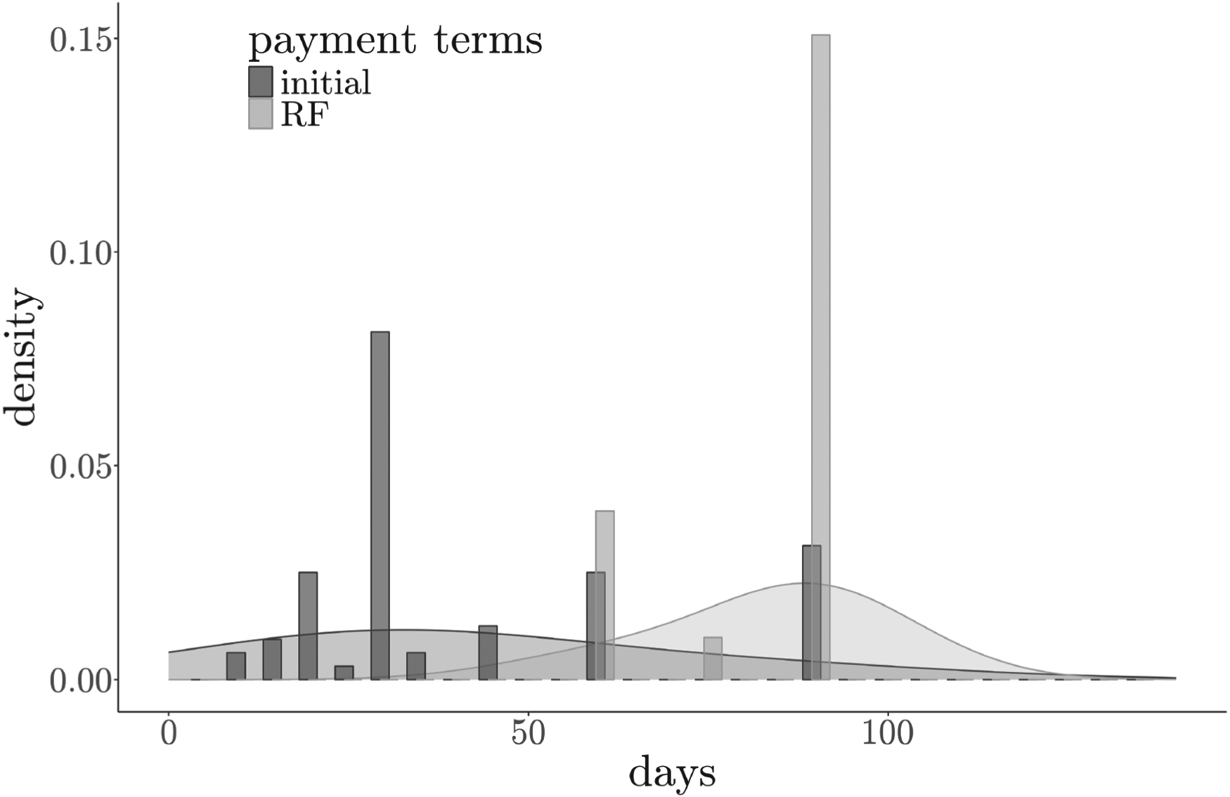
Table 2 provides summary statistics for the continuous variables (Table A2 in the Appendix provides demographic variables for the suppliers that did not adopt RF, suggesting no substantial differences). The variable payment term extensions captures the difference between RF payment terms and initial payment terms. In a few cases, buyers adopt RF even with shortening payment terms (i.e., negative extensions), but the mean is positive with
Summary statistics for continuous variables.
Note. Values reported in this table have not been transformed.
To operationalize standardization, we calculated each buyer’s most frequent RF payment term (e.g., 60 days). The variable standard RF terms assumes one for suppliers with RF payment terms equal to this value and zero otherwise. Its mean of 58.5% indicates that about one out of two suppliers obtained standard RF terms in our sample. For a robustness test, we also created a variable called standard initial terms that we define as “1” if the initial payment terms of a supplier and a buyer are equal to the mode of initial payment terms and “0” otherwise. Its mean of 38.9% describes that only about one of three suppliers had standard initial terms in our sample. Comparing both means is a crude indicator that adopting RF seems to lead to standardization, as we will test more carefully below.
The annualized risk-free rate averages 1.1%. Annual spend captures sales within the buyer–supplier dyad, whereas supplier revenue is a supplier’s entire revenue so that it may also originate from other buyers. These two variables are right-skewed, so we consider their logarithm in the subsequent analysis. RF interest rate averages about 2% and is an annualized value. Buyers tend to be larger than suppliers in our dataset, as reflected by a higher average buyer revenue. The variable buyer costs of goods sold indicates the importance of the buyers’ upstream supply chains. The RF program size variable reflects the number of suppliers in a buyer’s program, with an average size of 26 suppliers (=1,898/73). This variable is a snapshot at the end of the sample period and, thus, a proxy for the eventual importance of the RF program. Finally, the variable past RF suppliers count indicates the number of suppliers a buyer bargained with in the past. Although this variable is on the buyer level, there are 1,898 observations because it increases by 1 for each supplier. It is thus a dynamic value that differs from the RF program size. Because this count measure is right-skewed, we consider its logarithm.
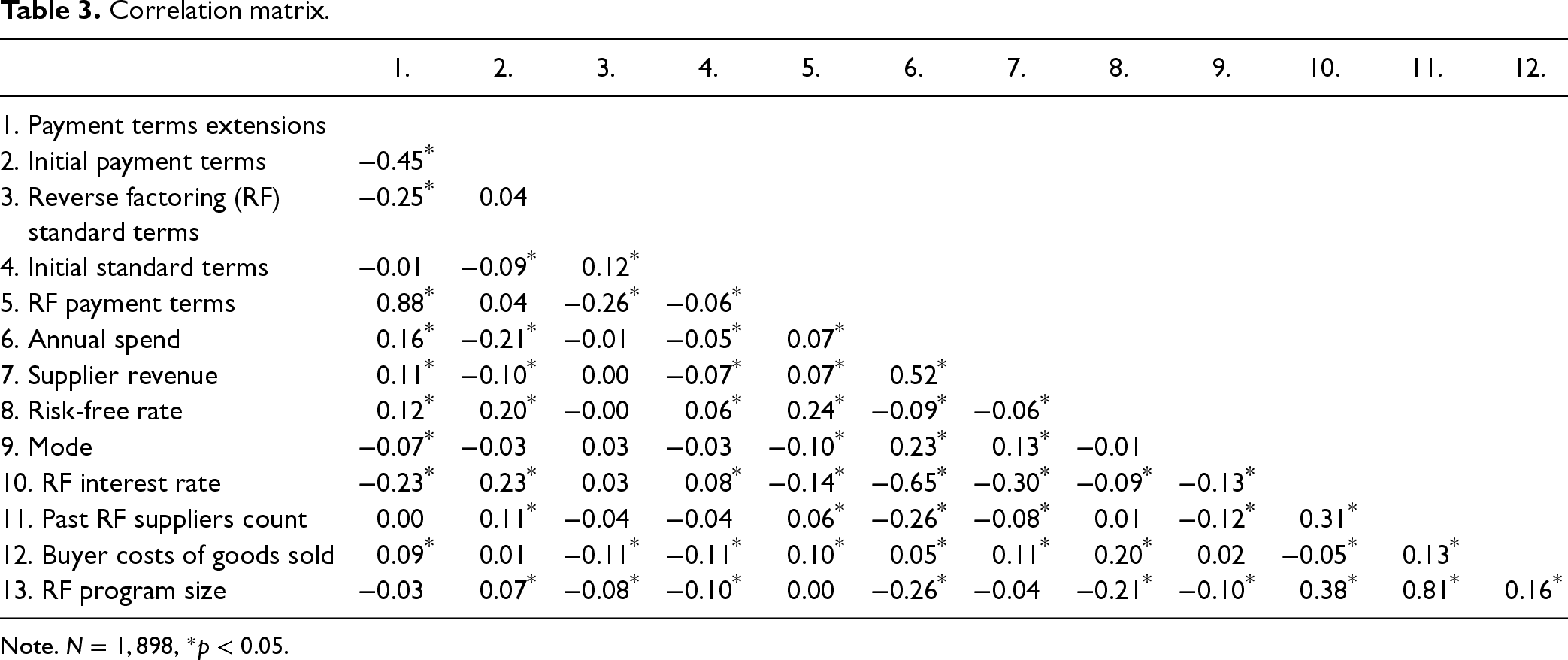
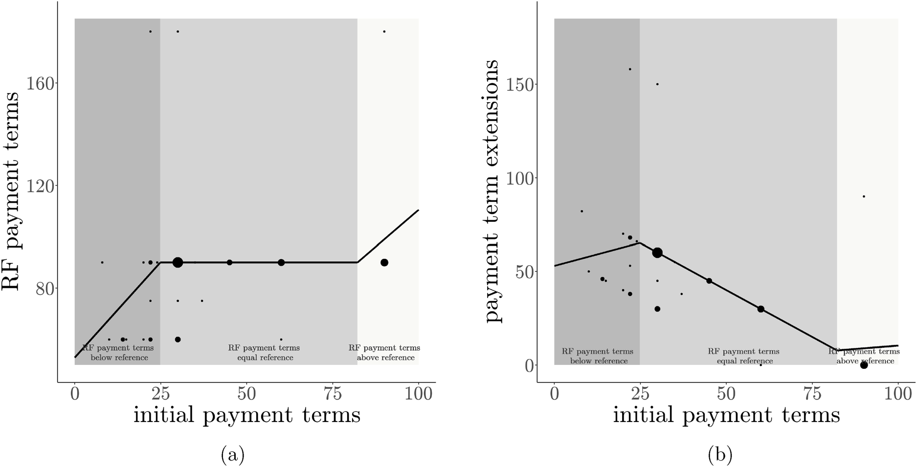
We scale all variables for the subsequent analysis (i.e., we mean-center each and divide it by its standard deviation) with two exceptions. We attain a more meaningful interpretation by keeping payment term extensions and initial payment terms untransformed. Because initial payment terms and RF payment terms are central in our analysis, we illustrate their distributions featuring one buyer that uses RF with 64 suppliers as an example. Figure 5 illustrates the distributions of initial payment terms and RF payment terms along with normal density plots.
Histogram and density of initial payment terms and reverse factoring (RF) payment terms for one example of a buyer with 64 suppliers.
Next, we describe our econometric strategy for testing our hypotheses. Section 5.3 provides complementary maximum likelihood estimates of a model that mimics the structure of the analytical model more closely. We test Hypothesis 1 using a paired 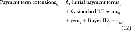
Several factors might affect both payment term extensions and initial payment terms. In a second linear model, we control for those,
Our dataset features data on 96 suppliers who decided against adopting RF. They give rise to selection bias concerns. We estimate a Heckman selection model to examine whether our estimates are biased because of selection effects. The following specification states the selection equation,
Correlation matrix.
Note.
Hypothesis 1 is supported
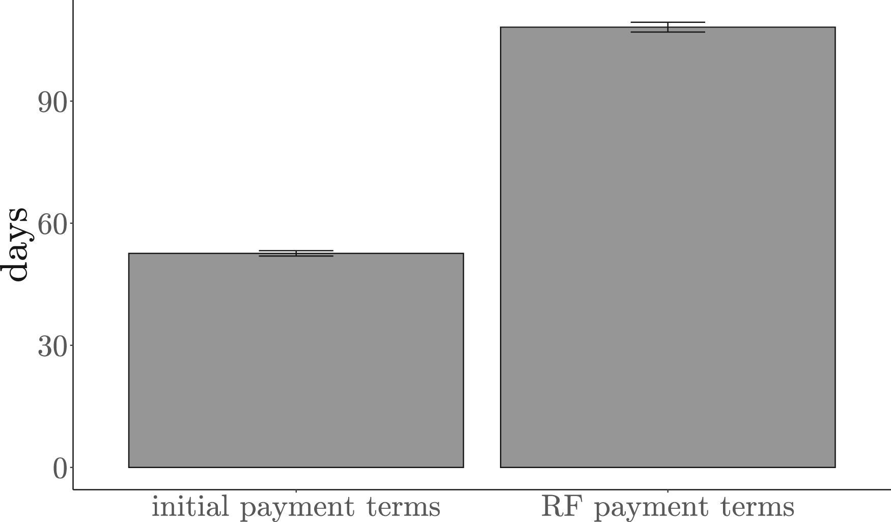
Bars indicate sample means, and whiskers indicate standard errors.
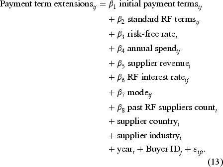
Turning to Hypotheses 2 and 3, Columns (1) and (2) in Table 4 provide the estimates for the specifications in equations (12) and (13), respectively. Adding the control variables in the second column increases the
OLS and Heckman selection estimation.
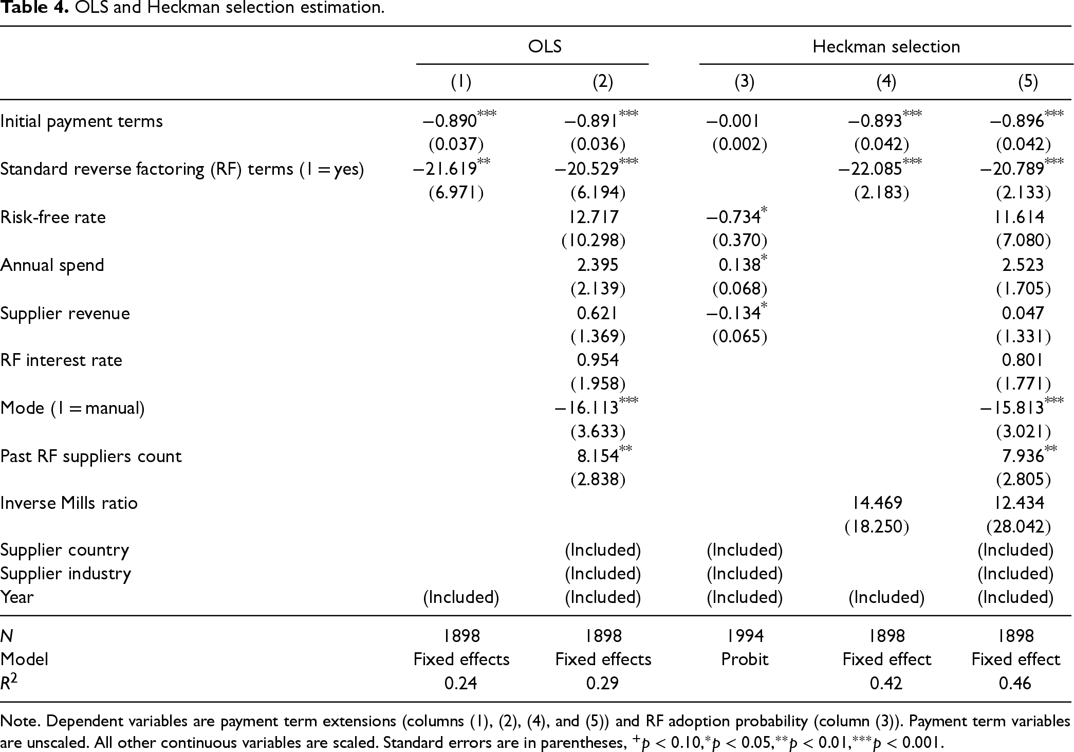
Note. Dependent variables are payment term extensions (columns (1), (2), (4), and (5)) and RF adoption probability (column (3)). Payment term variables are unscaled. All other continuous variables are scaled. Standard errors are in parentheses,
Hypothesis 2a is rejected, and Hypothesis 2b is supported, as seen by the significant and substantial negative effect of
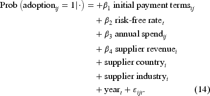
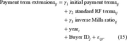
Column (3) estimates the selection equation, equation (14), while Columns (4) and (5) estimate the outcome equations equation (15) and equation (16), respectively. Column (3) suggests that suppliers are more likely to adopt RF when the risk-free rate is low
It is worthwhile to discuss some of the control variables. We will focus on the estimates in Column (2), noting that they, too, are consistent with their counterparts in Column (5). Recall that mode=1 indicates that suppliers use RF manually, that is, only on select invoices and convert their receivables into cash when needed, as opposed to mode=0, which refers to suppliers that use RF for all invoices immediately. As mode=1 provides more flexibility, suppliers should only use mode=0 if they need RF to a large extent and seek to avoid transaction costs that arise from managing each invoice individually. The estimates indicate 16 days shorter payment term extensions for manual suppliers (
Standardization is a central concept in our game theoretic analysis; it is a key complement to former RF studies. So, we studied it further through a series of hypotheses motivated by our analytical results. Figures 2(a), 4(a) and (b) suggest that initial payment terms should only result in standardized RF payment terms if they are within a specific interval (the medium gray-shaded area in those figures), which is not too broad. If true, this would imply that initial payment terms are more likely to become standardized if they are somewhere in the middle. To capture this idea more formally, take the subset of suppliers that obtain standard RF terms for each buyer. Then, consider the median initial payment terms of these suppliers. Centered on this median, consider intervals of varying width: The 0% interval only includes the median, the 10% interval comprises 10% of all initial payment terms symmetrically around the median, and so on, so that the 100% interval comprises all initial payment terms. We refer to these intervals as median-centered intervals. Now we can formulate the idea that initial payment terms more likely become standard terms if they are somewhere in the middle:
Hypothesis 4. The fraction of initial payment terms that become standard RF terms is negatively associated with the width of the median-centered interval that they are in.
To test this hypothesis, the first interval that we constructed has a width of 0%. In 69.4% of cases within this interval, payment terms became standard. Next, we examined the symmetric 5% interval to notice that still, in 67% of the cases, payment terms became standard. We continued this approach with intervals of increasing width as shown in Figure 7. The horizontal axis displays the interval width, and the vertical axis shows the percentage of initial payment terms that became standardized. The dashed line corresponds to the sample mean of 58.5%. When comparing smaller intervals with this overall average, we notice that observations in the 0% interval significantly more frequently led to standard terms (
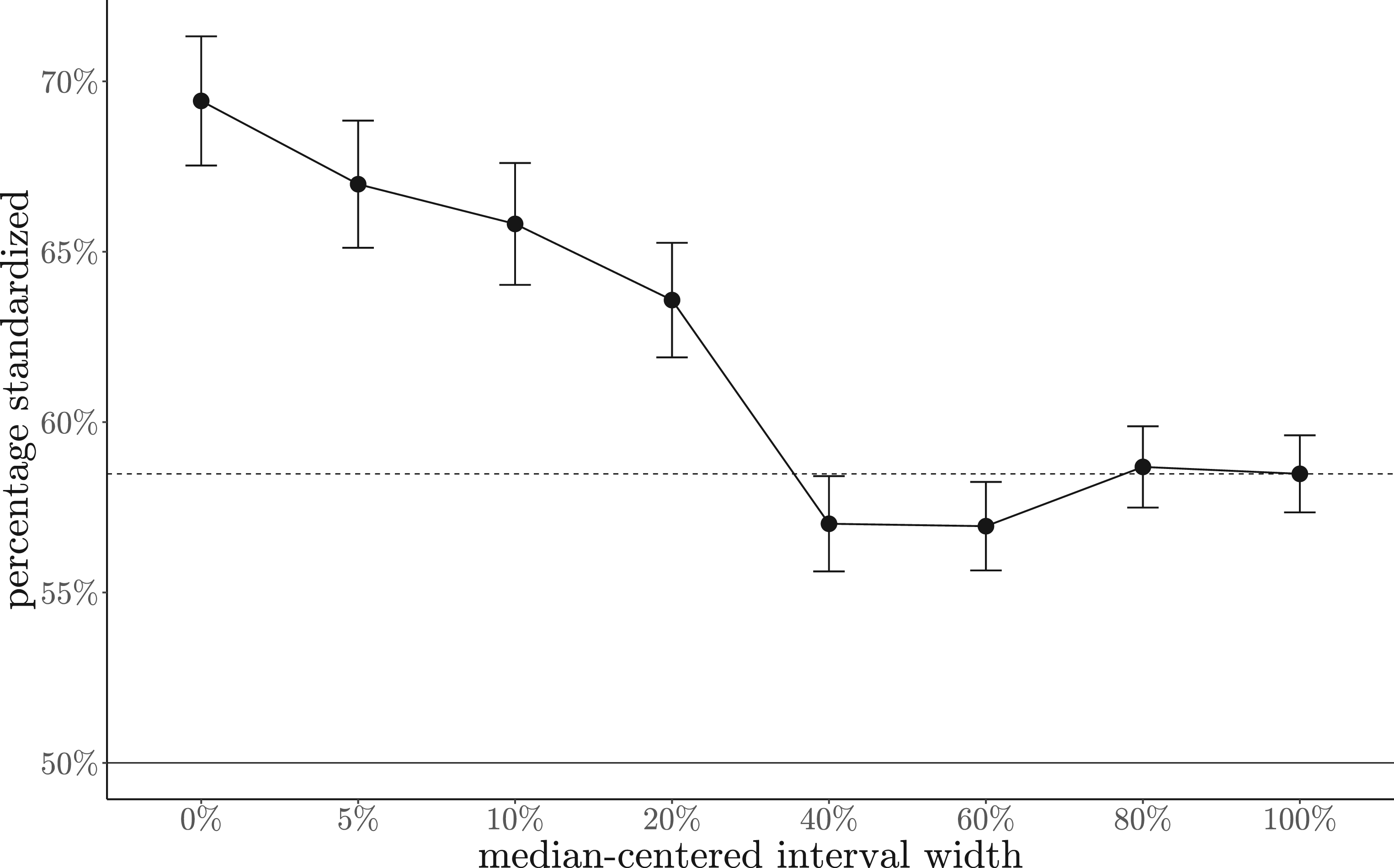
Standardization.
We conducted further analyses to examine the idea of standardization. To be consistent with our model, we would expect the payment terms to become more similar on the buyer level under RF. Formally,
Hypothesis 5a. The adoption of RF is negatively associated with the number of different values of payment terms on the buyer level.
To test Hypothesis 5a, we counted how many different terms each buyer had before adopting RF and after. Figure 8(a) provides the distribution and density of this count variable. Since this number is skewed, we took the logarithm. We tested whether this value was significantly reduced using a paired
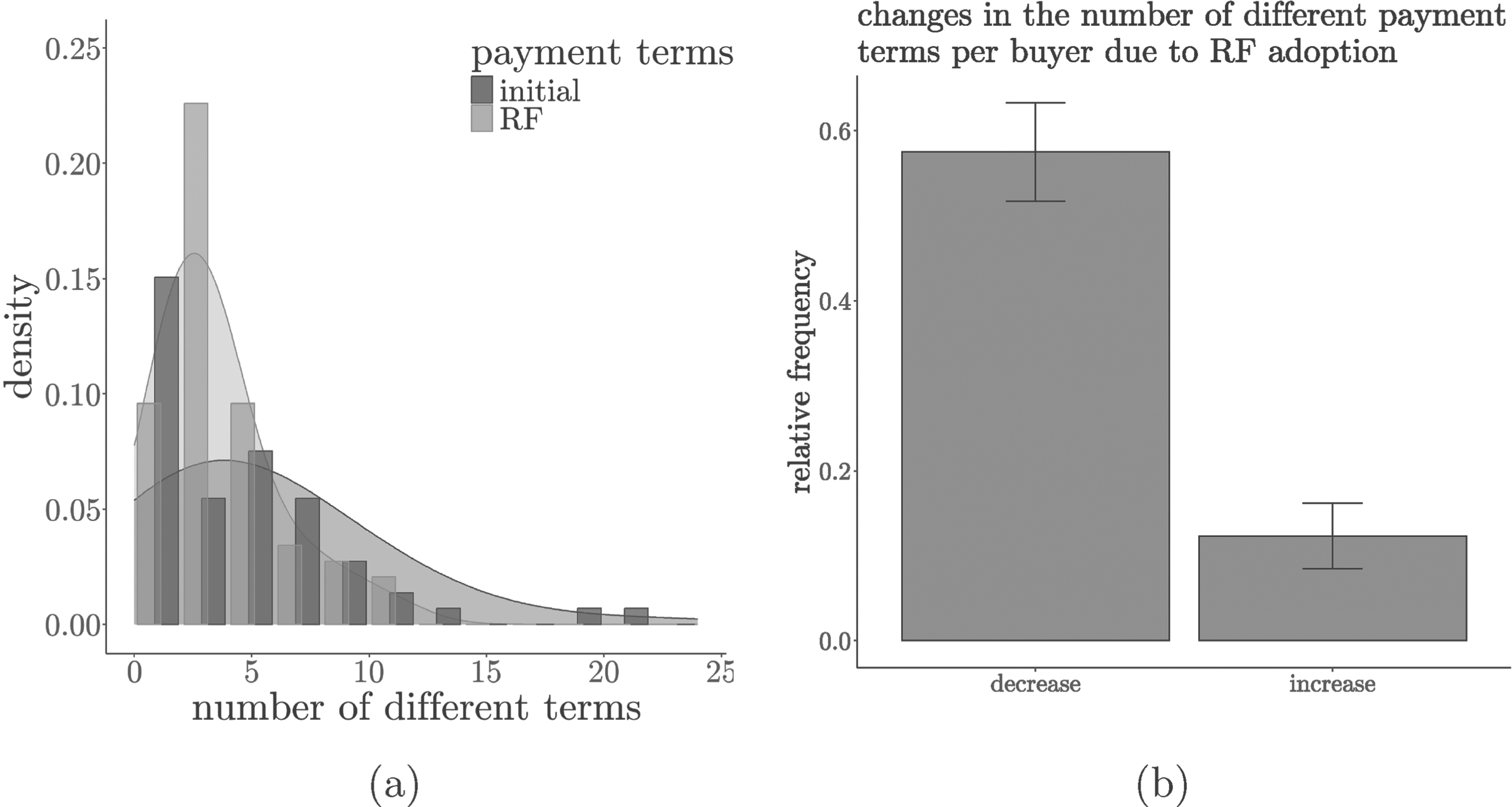
Standardization on the buyer-level,
Relatedly, we expect the standardization to be heterogenous across all buyers. Standard terms should be less salient in smaller programs. Buyers with larger RF programs might also have a stronger incentive to standardize terms. Formally,
Hypothesis 5b. RF program size is positively associated with payment terms standardization.
We created the binary variable reduction of different terms, which is one if the buyer reduced the number of different terms. We estimated probit models with the following specifications,
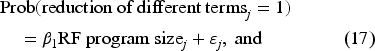
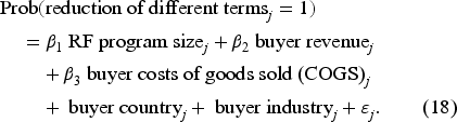
Probit regression on standardization.
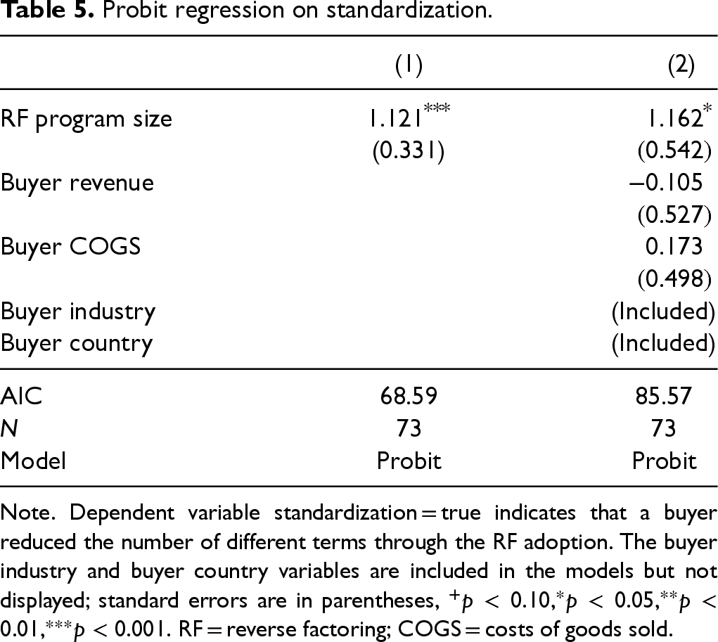
Note. Dependent variable standardization = true indicates that a buyer reduced the number of different terms through the RF adoption. The buyer industry and buyer country variables are included in the models but not displayed; standard errors are in parentheses,
One of our final tests examines the possibility of dynamic updates to standard terms. Buyers may start with a specific standard level (e.g., 90 days) and adjust it over time (e.g., to 120 days). If such adjustments occur, we would expect the number of different RF payment terms as a fraction of all newly added suppliers within a given year to be relatively small compared to the same fraction calculated across all years. We define the former as the mean fraction of different terms per year and the latter as the fraction of different terms overall. The value of 0 indicates that all terms in the same time frame are identical. Figure 9 visualizes this idea with a scatter plot where each dot represents one buyer. If dynamic updates were common, most points would lie above the 45-degree line, indicating higher standardization per year. However, this is not the case, suggesting that buyers generally do not adjust their standards dynamically.
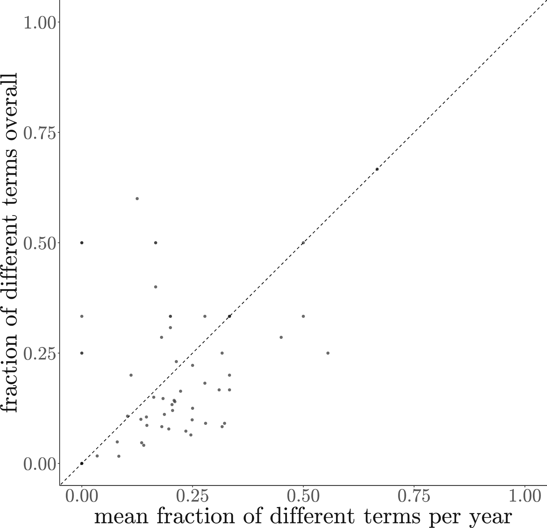
Scatter plot,
Although we do not seek to imply causality, we carried out a series of tests to examine whether endogeneity or modeling choices unduly affect the results.
The main finding of our analysis is the negative effect of initial payment terms on their extension. The variable initial payment terms might be endogenous. After all, initial payment terms might be affected by unobserved variables such as relationship type (strategic versus arms-length), mutual dependence, and power imbalance between a buyer and a supplier. Since we do not observe those variables, they are part of the error term,
We next constructed an instrumental variable. We created a set for each supplier that contains all other suppliers in the same country and industry and calculated their average initial payment terms. We called this variable country-industry average payment terms. This instrument is relevant because firms within the same country and industry tend to have similar payment terms. Further, the exclusion restriction applies to this instrument. As seen in equation (13), country-industry average payment terms does not appear in our model. In addition, country-industry average payment terms do not affect unobserved variables like relationship type, mutual dependence, and power imbalance. Vice versa, those variables do not affect the country-industry average payment terms. We then used an instrumental variable estimator with the following specifications.
In our dataset, there are 18 supplier-country-industry combinations that feature only one supplier. Since we could not calculate the variable country-industry average payment terms in those cases, we estimated the model on the remaining 1,880 observations (about 99% of the full sample). Column (1) in Table 6 shows the estimates of equation (19). The dependent variable is initial payment terms, and the effect of country-industry average payment terms is significantly positive, indicating relevance.
Robustness tests.
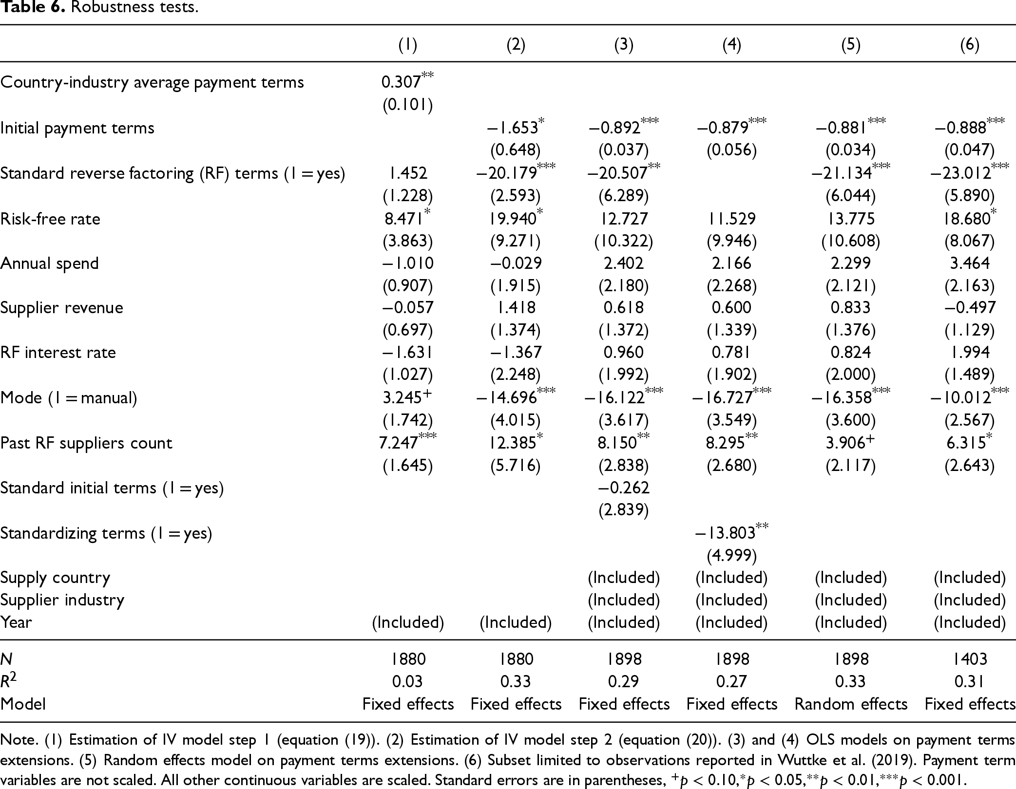
Note. (1) Estimation of IV model step 1 (equation (19)). (2) Estimation of IV model step 2 (equation (20)). (3) and (4) OLS models on payment terms extensions. (5) Random effects model on payment terms extensions. (6) Subset limited to observations reported in Wuttke et al. (2019). Payment term variables are not scaled. All other continuous variables are scaled. Standard errors are in parentheses,
Column (2) in Table 6 shows the IV estimates. Again, initial payment terms are negatively associated with payment term extensions (
Columns (3) and (4) present OLS estimates for models that depart from equation (13). In Column (3), we added the variable standard initial terms in the model. This variable captures whether payment terms have been standard before introducing RF. Neither is this variable significant nor does it substantially affect standard RF terms. As an alternative measure for the latter variable, we consider the variable standardizing terms, which is one if initial payment terms are not standard, but RF payment terms are. As Column (4) indicates, the results are robust with respect to this change
Finally, we examined whether there are non-linear effects of initial payment terms by considering second and third-order polynomials. When adding those terms to the main model and reestimating the model, those additional coefficients turned out to be insignificant. This is consistent with our theory, which does not predict polynomial relationships.
Our analytical model provides theoretical predictions (Section 3), which we translated into hypotheses and tested at the beginning of this section. This subsection complements the data analysis by estimating the unobserved fairness (
In this section, we use the hat symbol to indicate observed values. For observed initial payment terms,
We estimated the 5 parameters of each buyer. To maintain enough degrees of freedom, we included all buyers with at least 10 suppliers in their RF programs in this estimation procedure, corresponding to 32 buyers. Excluding buyers with relatively few suppliers, the sample still comprises 1,839 buyer–supplier dyads or 96.8% of all observations.
We then calibrated our model. Our dataset features the RF interest rate
Estimation Results
Figure 10 illustrates the estimates for one buyer (the same buyer as in Figure 5). Figure 10(a) shows the estimated slope for the equilibrium RF payment terms, Figure 10(b) shows the corresponding shape for the payment term extensions. In this example, standardization occurs for initial payment terms between
Empirical example of the same buyer with 64 suppliers as in Figure 5. Size indicates the number of suppliers. Solid lines indicate maximum likelihood equilibrium estimations. (a) The solid line is akin to the equilibrium curve in Figure 2(a). (b) the solid line is akin to the equilibrium curve in Figure 3.
In the case of the buyer in Figure 10, our model fits significantly better than the hyper-rational model (
Maximum likelihood estimation results for fixed power. (a)
The estimated value of fairness is notably high, being in the ballpark of interest rates. Economically, even this magnitude is plausible. For instance, a buyer extending payment terms from 90 to 100 days on a $100,000 annual spend at a typical 2% interest rate saves only $55 annually. Such savings may not justify the risk of perceived unfairness, which could harm buyer–supplier relationships. As one manager from a large manufacturing firm with a leading RF program noted, suppliers frequently cite fairness in negotiations. Experimental evidence, such as ultimatum games, further shows that fairness concerns often lead individuals to forgo significant value (Hoffman et al., 1996; Thaler, 1988). Further, the substantial effect of fairness aligns with our main linear model, which shows a strong negative relationship between initial payment terms and payment term extensions. At the same time, we also acknowledge these as point estimates, noting that true values may differ.
Subfigure 11(b) presents estimates for the standardization value for the buyer (
We focus our ensuing discussion on fairness (
Tests on estimated parameters,
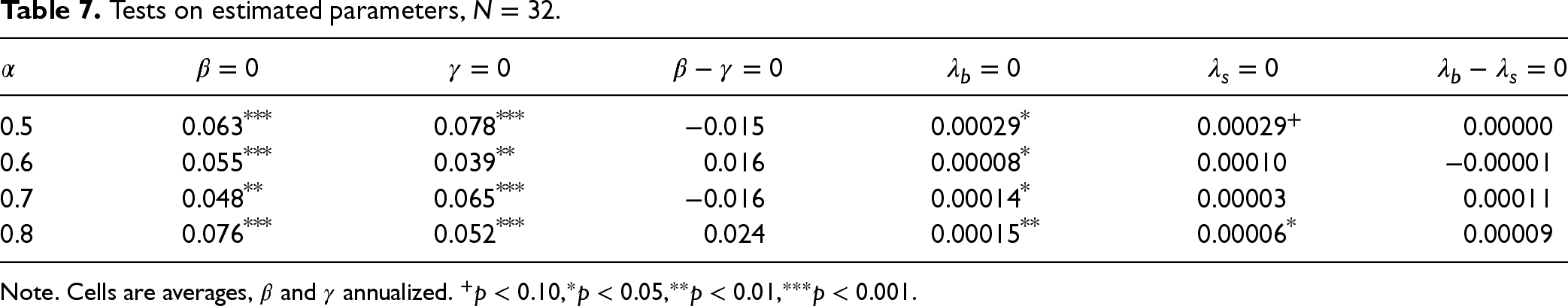
Note. Cells are averages,
We performed a counterfactual analysis to compare the relative importance of the three motives: Financing cost, fairness, and standardization. To that end, we consider an average RF program with an average buyer–supplier dyad. Consistent with our assumptions in this section and the sample averages, we thus assume
We began calculating the hyper-rational benchmark (see Proposition 1). For expositional clarity, we define profit functions for hyper-rational players, which are special cases of the utility functions in equation (1) for
We generated the counterfactual outcomes in two regards. First, we calculated hypothetical, hyper-rational profits
Counterfactual analysis.
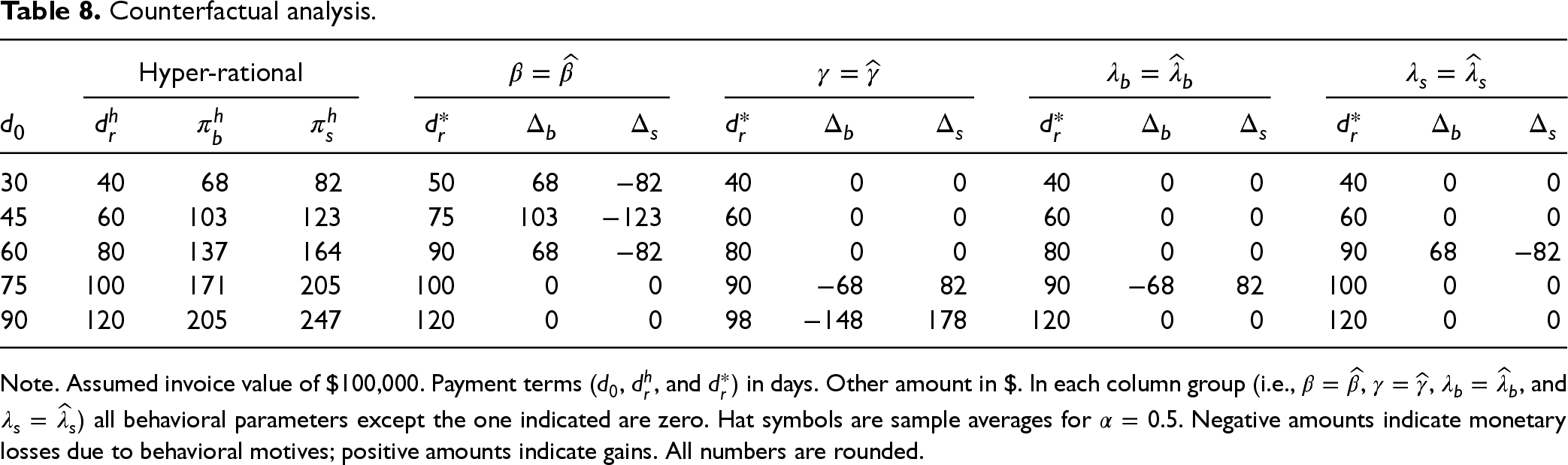
Counterfactual analysis.
Note. Assumed invoice value of $100,000. Payment terms (
Let us focus first on the effect of fairness and standardization on bargaining outcomes. As expected, the buyer’s fairness concerns,
Finally, we turn to the effect on hyper-rational profits. The buyer’s fairness concerns strengthen its bargaining position. Comparing columns
Our study’s key research question is how firms extend payment terms in the context of RF adoption. Our game-theoretical model features three motives and predicts how, if applicable, they would shape bargaining outcomes. We then derived and tested four hypotheses. So, are all motives present?
The rejection of Hypothesis 2a suggests that the financing cost motive is less dominant than expected. After all, buying firms mainly introduce RF to improve payment terms, and Hypothesis 2a is fairly consistent with extant models (e.g., Kouvelis and Xu, 2021; Lekkakos and Serrano, 2016; van der Vliet et al., 2015; Wuttke et al., 2016), so we would have expected longer payment term extensions for suppliers with longer initial payment terms; but this is not reflected in our sample. Support for Hypothesis 2b suggests the existence of the fairness motive. Accordingly, payment terms are not extended by more if they are already long, but by less—suppliers with long payment terms would find it unfair to extend them even more. Likewise, payment terms are extended by more for suppliers on shorter terms—buyers would find it unfair not to achieve an outcome comparable to other suppliers, given all suppliers obtain similar financing conditions with RF. In some cases, our model predicts standardization of payment terms, which happens more often than randomly (support for Hypothesis 5a). Further results, robustness tests, and structural estimation results lend additional support to the existence of all three motives.
Turning to managerial implications, we cannot say whether standardization is optimal, as witnessed in our dataset. Still, managers who ignore this facet seem ill-advised when crafting an RF and payment terms strategy. They are likely miscalculating their expected benefits. At the same time, managers who only focus on standardization might be underperforming as they deviate from profit-maximizing behavior, downplaying the financing cost motive. A careful assessment based on the buyer’s supply chain strategy can help. Our study also has implications for RF providers who often consult with (potential) clients before starting an RF program. Our results should be reflected in their work, and they should carefully differentiate between the potential effect on days payables outstanding (which is one of their top-sales arguments) and the supply chain effect (which requires a deeper understanding of standardization). Simple calculators anchored on financing costs can be misleading; fairness and standardization also matter.
Finally, as with all econometric studies, ours has some limitations. While we carefully address a series of potential endogeneity issues, it is always difficult to establish causality with secondary data. If future research could address three shortcomings, it would be valuable to treat selection biases thoroughly. Although we estimated a selection model, we only had information on 96 suppliers who declined an offer. Further selection biases can arise when RF providers do not offer RF programs to some buyers or buyers decide not to offer RF to some suppliers. Since all buyers and suppliers in our dataset use RF from the same RF provider, we cannot rule out idiosyncracies, and it is conceivable that buyers and suppliers might behave differently in other RF programs. Data from other RF providers could help to explore this. Second, we made simplified calibration assumptions in the maximum-likelihood estimation in Section 5.3 due to the lack of fine-grained data. Dyad-level and supplier-level data on further variables would strengthen the structural estimation. It might be possible for future research to collect such data for single RF programs, whereas we are not aware of any RF provider that collects such fine-grained data. Third, another aspect is the lack of causality in our tests. Our secondary dataset neither features direct fairness-related measures (
Supplemental Material
sj-pdf-1-pao-10.1177_10591478251319688 - Supplemental material for Empirical Evidence About Payment Term Extensions in the Reverse Factoring Context
Supplemental material, sj-pdf-1-pao-10.1177_10591478251319688 for Empirical Evidence About Payment Term Extensions in the Reverse Factoring Context by David Wuttke in Production and Operations Management
Footnotes
Summary statistics for continuous variables: Suppliers that did not adopt reverse factoring (RF).
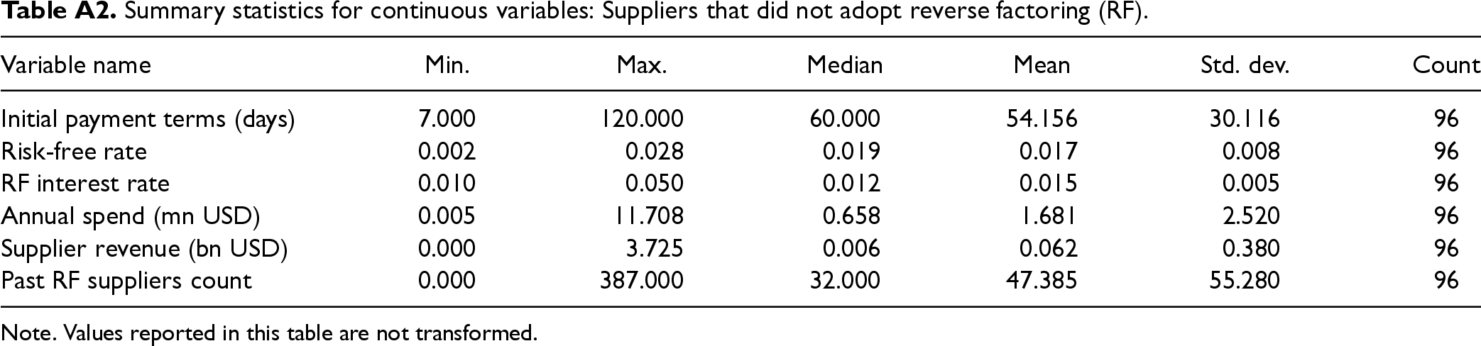
| Variable name | Min. | Max. | Median | Mean | Std. dev. | Count |
|---|---|---|---|---|---|---|
| Initial payment terms (days) | 7.000 | 120.000 | 60.000 | 54.156 | 30.116 | 96 |
| Risk-free rate | 0.002 | 0.028 | 0.019 | 0.017 | 0.008 | 96 |
| RF interest rate | 0.010 | 0.050 | 0.012 | 0.015 | 0.005 | 96 |
| Annual spend (mn USD) | 0.005 | 11.708 | 0.658 | 1.681 | 2.520 | 96 |
| Supplier revenue (bn USD) | 0.000 | 3.725 | 0.006 | 0.062 | 0.380 | 96 |
| Past RF suppliers count | 0.000 | 387.000 | 32.000 | 47.385 | 55.280 | 96 |
Note. Values reported in this table are not transformed.
Declaration of Conflicting Interests
The authors declared no potential conflicts of interest with respect to the research, authorship, and/or publication of this article.
Funding
The authors received no financial support for the research, authorship and/or publication of this article.
Notes
How to cite this article
Wuttke D (2025) Empirical Evidence About Payment Term Extensions in the Reverse Factoring Context. Production and Operations Management 34(9): 2579–2600.
References
Supplementary Material
Please find the following supplemental material available below.
For Open Access articles published under a Creative Commons License, all supplemental material carries the same license as the article it is associated with.
For non-Open Access articles published, all supplemental material carries a non-exclusive license, and permission requests for re-use of supplemental material or any part of supplemental material shall be sent directly to the copyright owner as specified in the copyright notice associated with the article.