
Abstract
Merchants use the rolling intrinsic policy to value commodity storage assets and monetize the values they attribute to these assets. A recent study ascribes to informational inconsistency two discrepancies between its partial monetization findings and the known excellent valuation performance of this method: (i) the rolling intrinsic policy can perform worse than the intrinsic policy and (ii) it appears to be far from optimal. This paper contends that this claim generally confounds informational inconsistency and the risk adjustment that underpins the common no-arbitrage valuation of this policy. In particular, lack of risk adjustment in that investigation explains at least the first difference and informational inconsistency cannot be associated with the second dissimilarity in about
Introduction
Merchant commodity trading companies acquire and operate commodity conversion assets to profit from commodity price differences in wholesale markets (see, e.g., Pirrong, 2014, 2015; Secomandi and Seppi, 2014, 2016; Secomandi, 2017; Lassander and Swindle, 2018; Trafigura, 2019). Gunvor, Mercuria, Trafigura, Vitol, and the trading units of major energy firms, such as British Petroleum, ExxonMobil, and Shell, are examples of such companies. Merchants need to (i) estimate the market values of commodity conversion assets when negotiating their acquisitions and (ii) make commodity trading and operating decisions when monetizing the values they ascribe to these assets after they have been acquired (see, e.g., Kaminski, 2012: Chapter 2; Secomandi, 2016). Because commodity prices are notoriously volatile, merchants often trade forward and other financial contracts to manage the risk of their profit and loss (P&L) profiles, that is, the payment of a commodity conversion asset acquisition cost and the stream of cash flows associated with trading around and operating this asset (see, e.g., Pirrong, 2014, 2015; Lassander and Swindle, 2018; Trafigura, 2019).
If one uses no-arbitrage valuation (see, e.g., Smith and McCardle, 1999; Bingham and Kiesel, 2004; Shreve, 2004; Guthrie, 2009, Luenberger, 2014: Chapters 14, 15, 19; Secomandi and Seppi, 2014: Sections 2 and 3; Babich and Birge, 2021: Section 3.3) to obtain a market value for a commodity storage asset and restricts attention to static policies then the intrinsic policy is optimal. Its no-arbitrage value is known as the intrinsic value of storage. The rolling intrinsic policy is a dynamic policy that sequentially reoptimizes the intrinsic policy. Merchants use it for both valuation and monetization purposes, in particular in the context of natural gas (see, e.g., Maragos, 2002; Gray and Khandelwal, 2004a, 2004b; Breslin et al., 2009; de Jong, 2016). This approach is part of commercial software (see, e.g., EnergyQuants, 2024; Lacima, 2024; Quantego, 2024), the subject of several studies (see, e.g., Lai et al., 2010; Secomandi, 2010, 2015; Secomandi and Seppi, 2014; de Jong, 2015; Mandl et al., 2022), and a benchmark for other methods (see, e.g., Nadarajah et al., 2015; Mandl et al., 2022). Other research on the rolling intrinsic policy develops a variant thereof to achieve improved performance (Wu et al., 2012) or broadens its applicability (e.g., to networks of transport and storage assets, Nadarajah and Secomandi, 2018, and virtual power plants, Biegler-König, 2020).
Lai et al. (2010), Secomandi (2010, 2015), and Mandl et al. (2022), hereafter LMS, S10, S15, and MNMG, investigate two different roles that the rolling intrinsic policy plays for merchant commodity trading firms: The support of commodity storage asset valuation decisions in LMS, S10, and S15 and commodity trading and inventory adjustment choices when monetizing the value of a storage asset in MNMG (LMS and S15 consider other policies in addition to the intrinsic and rolling intrinsic policies and MNMG also propose a data-driven method based on empirical risk minimization; see, e.g., Vapnik, 1998). LMS, S10, and S15 calibrate stochastic forward curve models to data and use them in conjunction with no-arbitrage valuation to both value the intrinsic and rolling intrinsic policies and compute the optimal value of storage or estimates of upper bounds on it. MNMG employ observed forward curves for multiple nonoverlapping years to estimate both the expected values of these policies and an upper bound on the optimal expected value of storage. The values that LMS, S10, and S15 obtain embed an adjustment for market price risk, wheres the ones that MNMG determine do not. LMS, S10, S15, and MNMG restrict attention to spot trades.
LMS, S10, and S15 find that the rolling intrinsic policy is (i) considerably more valuable than the intrinsic policy and (ii) near optimal. Moreover, S15 establishes that the rolling intrinsic policy cannot have a no-arbitrage value that is smaller than the intrinsic one. MNMG reports that the rolling intrinsic policy (i) performs worse than the intrinsic policy in 37% of the instances that they consider and (ii) has an expected value that on average is 11% of the upper bound on the expected value of an optimal policy that they estimate. MNMG attribute these discrepancies to informational inconsistency between the true model of the data and the assumed ones that LMS, S10, and S15 calibrate to data.
This paper argues that the MNMG’s attribution to informational inconsistency of the two stated discrepancies generally confounds two aspects: (i) The errors associated with assuming a model of the data and calibrating it to a finite set of observations and (ii) the risk adjustment that ensues when applying no-arbitrage valuation. Whereas the steps in (i) lead to bona fide mistakes, the one in (ii) is a property of this valuation approach. As shown herein, both differences can arise when there is no informational inconsistency, in which case they are solely due to the absence of risk adjustment in the true model of the data and the presence thereof in the one used for no-arbitrage valuation. If the MNMG’s backtest featured risk adjustment in a way congruous with what no-arbitrage valuation assumes then at least the first deviation would not occur, even if informational inaccuracy existed. Moreover, the second discrepancy cannot be due to informational inconsistency in roughly
MNMG suggest extending their backtest of the intrinsic and rolling intrinsic policies by considering the versions of these policies that also trade forward contracts. This paper shows that in this case the first discrepancy can never occur, a result that ensues from the following improvement property established here: the rolling intrinsic policy cannot perform worse than the intrinsic policy on any forward curve trajectory when both of these policies are augmented with forward trading. This finding is known in practice (Gray and Khandelwal, 2004a: 1) but there is no formal proof of its validity in the literature. Moreover, it subsumes Proposition 2 of S15, which is restricted to no-arbitrage valuation and is not a sample path result. In general, as this paper illustrates, the second discrepancy can happen when the rolling intrinsic policy also trades forward contracts. Additional research could investigate if considering forward trading affects it in the context of the MNMG’s backtest (it cannot change the results of LMS, S10, and S15).
The backtest of MNMG implies that monetizing the value of a storage asset by operating it according to the rolling intrinsic policy without forward trading can yield monetization losses on average even if this asset were acquired at its intrinsic value or for free. In contrast, the improvement property shown herein implies that executing the forward trades of this policy provably eliminates these losses irrespective of the forward curve realizations if a storage asset can be purchased at no more than its intrinsic value, which is, however, unlikely to be the case. An investigation of the literature indicates that if the cost of such an asset is instead the assessed no-arbitrage value of the rolling intrinsic policy then this risk management approach leads to small monetization losses on average when applied to realistic instances. It also points to alternative and potentially better monetization techniques. This analysis encourages future research in this area.
Section 2 introduces background material. The discussions of informational inconsistency and risk adjustment in the context of the two discrepancies, the impact of forward trading on these differences, and the P&L risk management role of this activity are in Sections 3, 4, and 5, respectively. Section 6 summarizes this work and outlines future research, also considering both a third discrepancy and a notion of generalization error that MNMG associate with the rolling intrinsic policy.
Background Material
This section describes the commodity storage and trading setting in Section 2.1, introduces the intrinsic and rolling intrinsic policies in Section 2.2, and discusses the objective functions that LMS, S10, S15, and MNMG use in Section 2.3. The presentation relies on the notation of MNMG for the various quantities, with a minor modification of the definition of the set of dates, and adds the notion of risk-free discount factors with corresponding notation.
Storage and Trading
Consider a commodity storage asset managed on a merchant basis during a finite and discrete time horizon. This asset features minimal and maximal inventory restrictions, as well as limits, inefficiencies, and marginal costs for periodic inventory adjustments.
The time horizon includes the
Increasing or decreasing the inventory level by an amount
For date
Intrinsic and Rolling Intrinsic Policies
The intrinsic and rolling intrinsic policies prescribe commodity trading and inventory adjustment decisions based on optimal solutions to the intrinsic linear program (ILP), which is now specified.
Consider formulating ILP at time
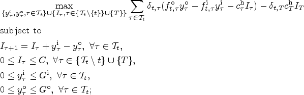
here the objective function to be maximized uses the forward curve and the operational costs to assign monetary values to the inventory adjustment decisions, which are associated with trading the commodity, and the resulting inventory levels; the first constraint set defines the dynamics of the inventory level; and the remaining sets of constraints ensure feasibility of both this level and its modification over time. The intrinsic value of storage for a given time and fixed inventory level and forward curve is the optimal value of the corresponding ILP objective function. The intrinsic value of storage without reference to a time corresponds to this value on the initial date (typically with zero inventory in storage). The name of this value derives from the fact that the model on which it is based ignores uncertainty.
The intrinsic policy uses an optimal inventory adjustment solution of ILP formulated on the initial date for the given inventory level and forward curve. Let this solution be
Similar to the intrinsic policy, one can implement the rolling intrinsic policy by making solely spot trades or supplementing them with forward transactions. Let
Objective Functions
LMS, S10, and S15 consider the intrinsic and rolling intrinsic policies as feasible ones for Markov decision processes (MDPs) that optimize the no-arbitrage value of storage. No-arbitrage valuation is also known as risk-neutral valuation because it amounts to taking the expectation of total cash flows discounted based on the risk-free interest rate under probability distributions modified so that the prices of futures are martingales that converge to the spot prices at their respective maturities. Notwithstanding the alternative name of this methodology, this martingale condition imposes an adjustment for market risk in the resulting valuations (see, e.g., Smith and McCardle, 1999). That is, although the probability distributions that no-arbitrage valuation uses are known as risk neutral, they are risk-adjusted versions of the ones employed to describe the actual dynamics of market prices. In the absence of arbitrage in financial markets, no-arbitrage values are unique if markets are complete, which means that every stream of cash flows can be replicated by dynamically trading financial securities, but otherwise they may not be so, because there is a single risk-adjusted probability distribution in the former case and infinite ones in the latter case.
MNMG employ an MDP that maximizes the expected value of the total storage and trading cash flows. This approach does not embed any adjustment for market risk because the interest rate is set to zero. One can thus proceed by assuming that in the MNMG’s procedure discounting is done using the risk-free interest rate.
The Two Discrepancies: Informational Inconsistency and Risk Adjustment
Informational inconsistency between the true model and an assumed model of the data can affect the magnitudes of the optimality gaps of the intrinsic and rolling intrinsic policies obtained with the former model under discounted expectation and the latter model under discounted risk-adjusted expectation (no-arbitrage valuation). However, if informational inconsistency were the only reason for the two discrepancies then they should disappear if this inconsistency were absent. Example 1 shows that this assertion is false for a perfectly efficient storage asset (
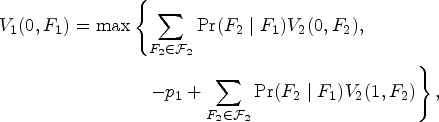
Consider an instance with three decision dates (
Figure 1 illustrates the evolution of the forward curve as a trinomial lattice. The starting forward curve ( Forward curve evolution for Example 1.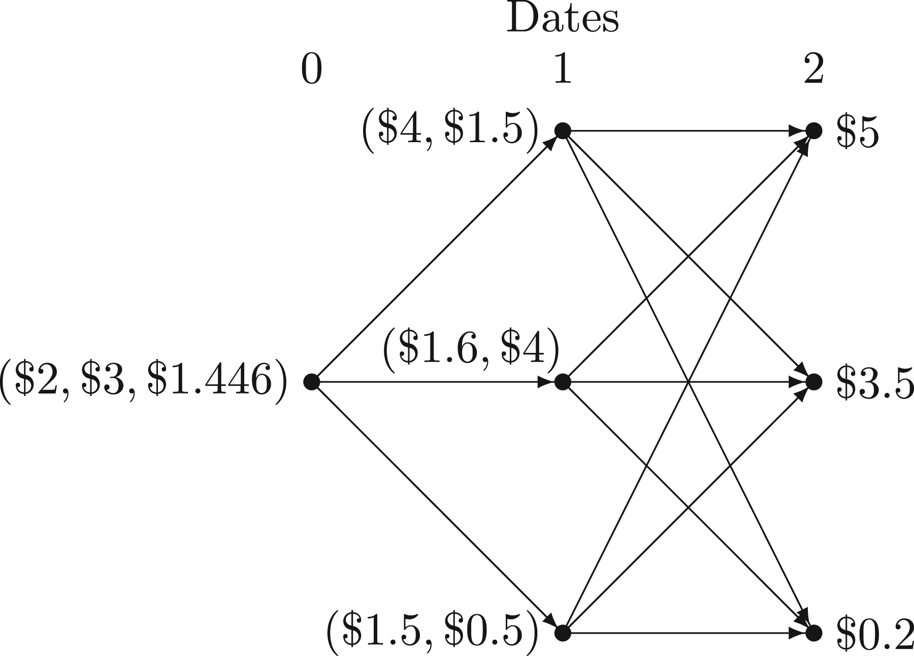
Consider implementing the intrinsic and rolling intrinsic policies by trading only in the spot market. The intrinsic policy buys one unit of commodity on the first date and sells it on the second date. The rolling intrinsic policy initially behaves as the intrinsic policy. If the realized forward curve on the second date is
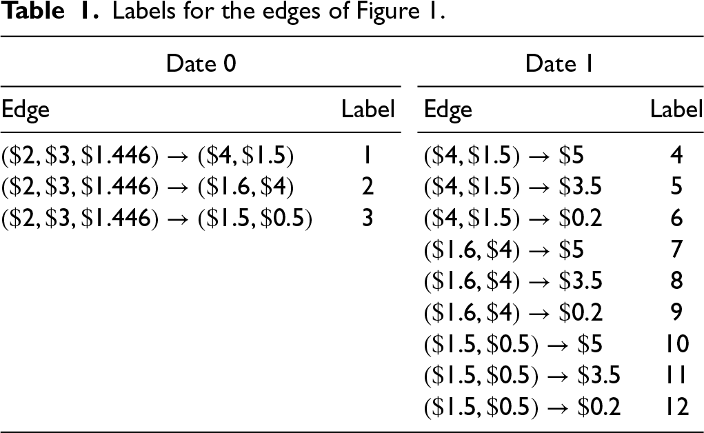
Labels for the edges of Figure 1.
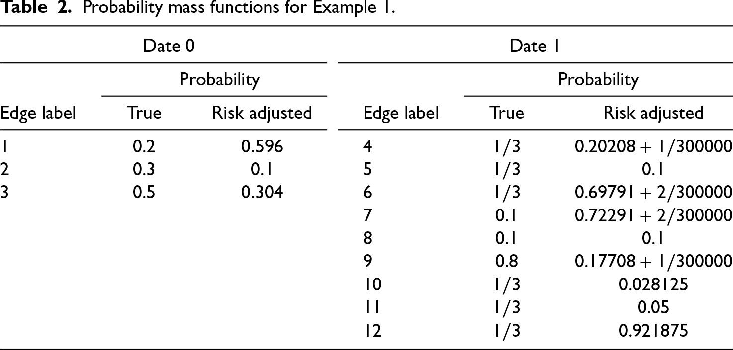
Probability mass functions for Example 1.
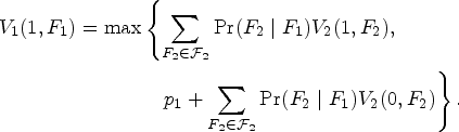
Expected and no-arbitrage values of the intrinsic, rolling intrinsic, and optimal policies restricted to spot trading for Example 1.
Example 1 recreates the two differences in the absence of informational inconsistency. Thus, in attributing them to this inconsistency MNMG include in it both modeling inaccuracies and risk adjustment, even if the latter element is a defining characteristic of no-arbitrage valuation. Put differently, although this methodology does distort the probability distribution associated with an assumed model to enact risk adjustment, this distortion is not inherently wrong. What can be erroneous (informationally inconsistent) is instead the model to which this change is applied, in which case a risk-adjusted probability distribution would reflect the model inaccuracies.
Proposition 2 of S15 states that under any risk-adjusted probability distribution, the no-arbitrage value of the rolling intrinsic policy cannot be lower than the intrinsic value of storage. If the risk-free interest rate is deterministic, which is the case in S15, the initial forward prices are the corresponding risk-adjusted expectations of the spot prices for the various maturities for any risk-adjusted stochastic model of the forward curve evolution. Thus, Proposition 2 of S15 continues to hold if the intrinsic value is replaced by the no-arbitrage value of the intrinsic policy, because in this case these two values coincide. In other words, the lack of risk adjustment in the true model of the data is a necessary condition for the existence of the first discrepancy irrespective of whether the model used for no-arbitrage valuation exhibits informational inconsistency. Therefore, the forward curves of the MNMG’s instances that give rise to the first discrepancy do not exhibit risk adjustment, an aspect that MNMG would label as informational inconsistency between this data and the models used by LMS, S10, and S15.
Example 1 in Online Appendix A of S15 illustrates a pathological case in which under no-arbitrage valuation the optimality gap of the rolling intrinsic policy is 100%. Thus, the lack of risk adjustment in the true model of the data is not a necessary condition for the occurrence of the second discrepancy in general. However, the discussion of informational inconsistency that MNMG provide, p. 2444, suggests that lack of risk adjustment in their backtest may play an active role in the occurrence of the second discrepancy. Moreover, informational inconsistency cannot be relevant in the one-twenty-fourth (around 4%) of their instances that feature a fast and frictionless asset (recall from the opening paragraph of this section that in this case the rolling intrinsic policy is optimal in the context of no-arbitrage valuation no matter which risk-adjusted probability distribution one uses).
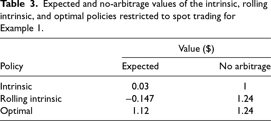
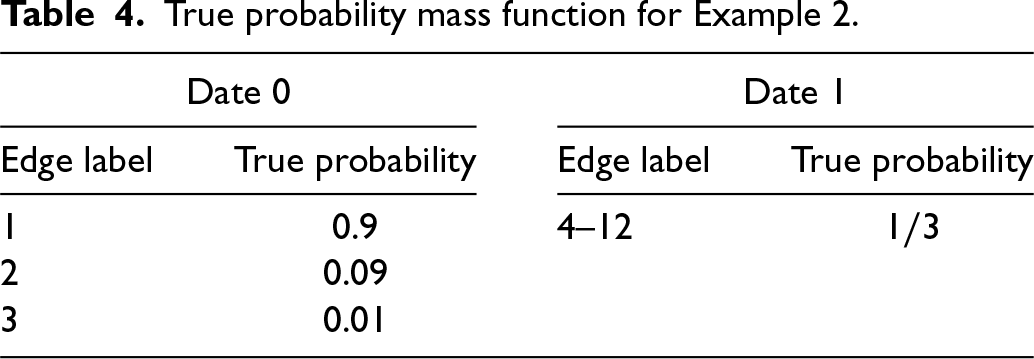
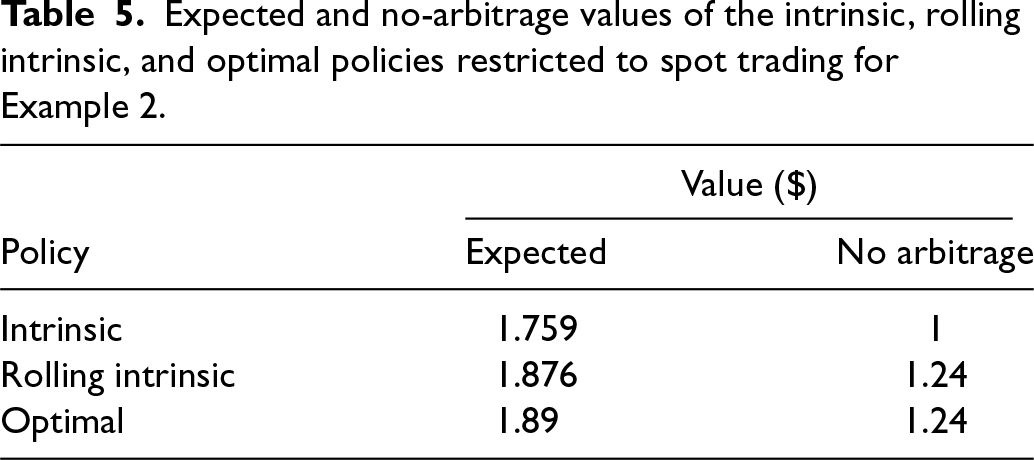
In general, the absence of risk adjustment in the true model of the data is not a sufficient condition for any one of the two discrepancies. Example 2 illustrates this statement when there is no informational inconsistency by modifying the true probability distribution that Example 1 employs.
True probability mass function for Example 2.
Expected and no-arbitrage values of the intrinsic, rolling intrinsic, and optimal policies restricted to spot trading for Example 2.
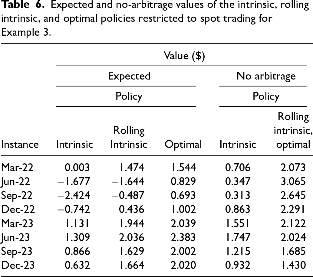
Example 3 deals with a more realistic setting than Examples 1 and 2 do. As these examples, it considers a fast and frictionless storage asset and does not feature informational inconsistency, but it uses eight instances that are partially based on prices of natural gas, an energy commodity that is part of the MNMG’s backtest, observed at Henry Hub, Louisiana during 2022–2023. Henry Hub is the main location for natural gas trading in North America. It is the delivery point of the natural gas futures traded on the New York Mercantile Exchange (NYMEX), which is part of the Chicago Mercantile Exchange. Henry Hub thus features a vibrant wholesale market. The findings of Example 3 largely reproduce in three and the remaining five of the considered instances the performance that the rolling intrinsic policy exhibits in Examples 1 and 2, respectively, when compared to optimal expected values (by construction it is optimal under no-arbitrage valuation). Further, with the exception of one statistic, they are broadly consistent with the ones that MNMG obtain for this policy in the natural gas component of their backtest.
This example encompasses instances based on both Henry Hub natural gas price data and a stochastic model of spot price changes calibrated to part of this data.
A mean-reverting model is commonly employed to describe the stochastic evolution of natural gas spot prices (see, e.g., Jaillet et al., 2004; S10), as well as the prices of other commodities (see, e.g., Schwartz, 1997). In the single factor formulation of Schwartz (1997), this model features three parameters: the (natural logarithm of the) mean reversion level, the speed of mean reversion, and the volatility, which amplifies random Gaussian shocks for the changes of the natural logarithm of the price (see Gambaro and Secomandi, 2021 and references therein for versions of this model with more realistic shock specifications than this one). This example makes the same assumption. Further, it calibrates the parameters of this model to Henry Hub spot prices observed from 1 January 2022 through 31 December 2023 by applying the approach described in Guthrie (2009: Section 12.1.2) with time increment set to 1 divided by 365.
Focus on a fast and frictionless natural gas storage asset situated at Henry Hub. The considered instances correspond to eight versions of this asset with 12 monthly decision dates and start dates corresponding to the first day of March, June, September, and December in both 2022 and 2023 (the choice of these dates is consistent with the ones of LMS and S15). The first three letters of these months combined with either 22 or 23 using a dash are the labels for the instances, for example the label of the March 2022 instance is Mar-22.
For each instance, the forward curve includes the Henry Hub spot price and the closing prices of the first 11 NYMEX natural gas futures for the instance initial date. Moreover, the risk-free interest rate is the United States Treasury Bill spot rate for this time. Commodity trading and inventory adjustment decisions are made at the beginning of each month.
The dynamics of the spot prices are represented as binomial lattices with true probabilities computed as explained in Guthrie (2009: Section 12.1.2) setting the time increment equal to 1 divided by 12. Scaling these probabilities using date-dependent factors without altering the support of the spot price distributions to match the forward curve observed on the start date of each instance yields the risk-adjusted probabilities (in contrast Jaillet et al., 2004 fix the risk-adjusted probabilities and scale the spot prices based on analogous factors). If a scaled true probability exceeds 1 then the corresponding risk-adjusted probability is set equal to the true probability. Further, the scale factor is recomputed. This process is repeated until all the scaled true probabilities are valid. This procedure yields legitimate risk-adjusted probability distributions for all eight instances.
Applying the stochastic dynamic program introduced in Example 1 to the setting of the present example yields the optimal policies and their values. The rolling intrinsic policy coincides with the resulting optimal policy in the no-arbitrage valuation case, because the storage asset is fast and frictionless. The intrinsic policy and value can be obtained using a deterministic version of the stochastic dynamic program discussed in Example 1 in which the initial prices of the forwards with maturities corresponding to the different dates take the place of the spot prices at these times. In particular, the chosen risk-adjusted probabilities ensure that evaluating the intrinsic policy on the constructed binomial lattices yields the intrinsic value determined using only the forward curve. Hence, comparing the computed values of the intrinsic and rolling intrinsic policies is meaningful. (An alternative approach to obtain an optimal policy under no-arbitrage valuation, and hence the rolling intrinsic policy, is to use the optimal decision rules that Proposition 1 in S15 states. Further, a straightforward modification of these decision rules yields the intrinsic policy, because it is an optimal static policy in this case.)
Expected and no-arbitrage values of the intrinsic, rolling intrinsic, and optimal policies restricted to spot trading for Example 3.
MNMG, p. 2446, assert that supplementing the rolling intrinsic policy with forward trades eliminates negative expected (discounted) values. Proposition 1 states that augmenting this policy with the trading of forward contracts as described in Section 2.2 has an additional benefit: It ensures that the sum of the resulting discounted cash flows exceeds the corresponding sum for the intrinsic policy also implemented with forward trading irrespective of the forward curve realizations. This result assumes that the discount factors are based on the risk-free interest rate, which can be relaxed to assume that the intrinsic and rolling intrinsic policies use the same discounting approach.
On any given trajectory of the forward curve the sum of the total cash flows of the rolling intrinsic policy that also trades forward contracts discounted using the risk-free interest rate cannot be lower than the one of the analogous version of the intrinsic policy.
Recall from Section 2.2 that the suffix 
The time 0 discounted optimal value of the objective function of ILP solved on date 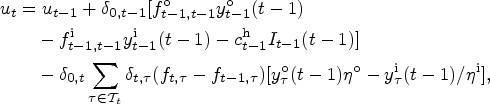
At time 
that is, 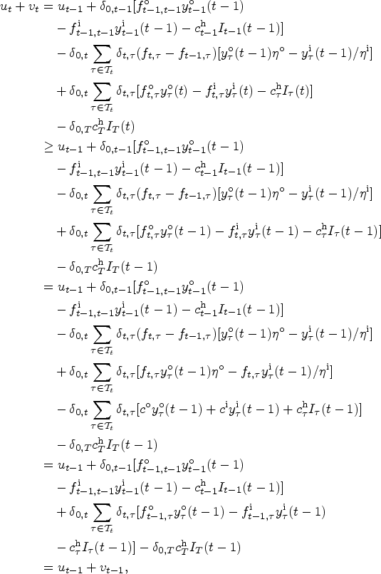


Proposition 1 stated with the sum of the total discounted cash flows of the intrinsic policy augmented by forward trading replaced with the intrinsic value of storage is familiar to practitioners and its proof formalizes the typical argument that they use to support it (Gray and Khandelwal, 2004a: 1). To gain some intuition on the rationale behind this result, pick a feasible inventory level and a forward curve pair (a state) on an arbitrary date excluding the initial and the last decision ones. Executing the inventory adjustment action corresponding to the forward contract that matures at this time and committing to keep all the other forward positions until their respective maturities is equivalent to unwinding all the forward positions, performing the same operating decision on the spot market, and both taking identical forward positions for all the remaining maturities at the new forward prices and pledging to hold them until their associated maturities. Thus, if the new intrinsic value exceeds the current value of the corresponding parts of the ILP optimal solution obtained on the earlier date and state then it is beneficial to (i) unwind the previous forward positions and (ii) both adjust the inventory in the spot market and update the forward positions for the outstanding maturities according to the new ILP optimal solution rather than to adhere to the relevant part of the incumbent ILP optimal solution. Applying the same logic along an entire trajectory of the forward curve results in a sum of total discounted cash flows that is at least as large as the intrinsic value, because on each date a weak improvement occurs.
The property that Proposition 1 states holds with probability 1. Thus, it is true in expectation under any stochastic model of the evolution of the forward curve. Corollary 1 gives this result under the same assumption that distinguishes Proposition 1 (it can be relaxed in a fashion analogous to what is indicated for this proposition).
Under discounting based on the risk-free interest rate, the mean of the sum of the total discounted cash flows of the rolling intrinsic policy augmented with forward trading cannot be lower than the intrinsic value of storage.
Corollary 1 subsumes Proposition 2 of S15 despite the fact that S15 does not consider forward trading, because S15 uses no-arbitrage valuation under which this activity has zero value. Example 1 includes an illustration of this statement.
It follows from Corollary 1 that the first discrepancy cannot occur when the intrinsic and rolling intrinsic policies also trade forward contracts. Example 4 illustrates this conclusion. It also shows that in general the second discrepancy can happen when the rolling intrinsic policy trades forwards. For ease of exposition, hereon
Consider the setting of Example 1.
The intrinsic policy that also trades forward contracts buys one unit of commodity spot on the first date, increases the inventory accordingly, sells this unit forward for delivery on the second date, and commits to using this inventory amount to deliver against this forward position at this time. The corresponding cash flows are −$2 initially and $3 on the second date no matter what the forward curve realization is. The sum of these cash flows is $1 with probability 1. The intrinsic value of the asset is thus
On the initial date the rolling intrinsic policy augmented with forward trades makes the same choices as the analogous version of the intrinsic policy. For the remaining dates three cases need to be considered.
Case 1. If the realized forward curve on the second date is
Case 2. If the forward curve observed on the second date is
Case 3. If the observed forward curve that occurs on the second date is
Expected and no-arbitrage values of the intrinsic and rolling intrinsic policies with forward trading, optimal expected and no-arbitrage values with spot trading, and upper bounds on the extended Markov decision process (MDP) optimal policy expected value for Example 4.
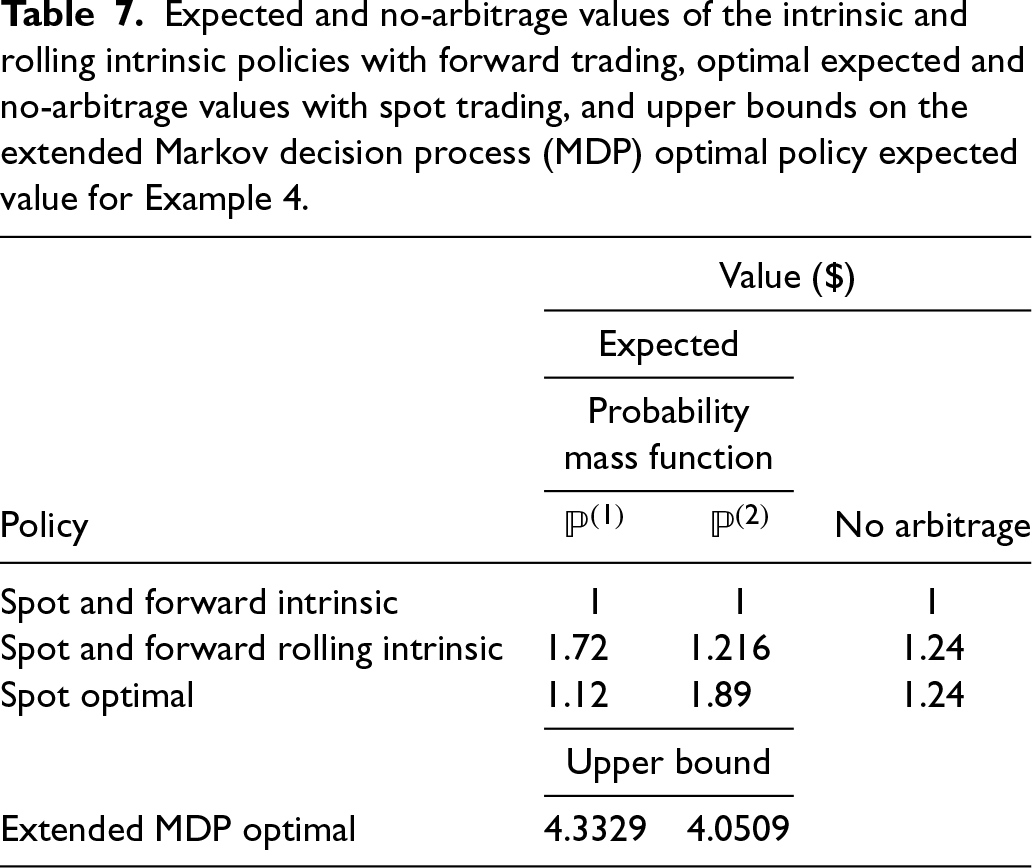
In Example 3 the extent of the second discrepancy at a minimum substantially reduces when the rolling intrinsic policy trades forward contracts (this statement hinges on comparing the fourth and fifth columns of Table 6 for the Jun-22, Sep-22, and Dec-22 instances in light of Corollary 1). Regarding how the inclusion of forward trading may affect the second discrepancy in the context of the LMS, S10, S15, and MNMG studies, the results of LMS, S10, and S15 remain the same, because trading forwards has zero no-arbitrage value, whereas the findings of MNMG will change at least for the instances associated with the first discrepancy. Moreover, a proper assessment of the optimality gaps of the rolling intrinsic policy requires considering the extended MDP, as done in Example 4.
The P&L associated with managing a storage asset on a merchant basis includes the initial outflow for purchasing the asset and the sum of the discounted stream of subsequent commodity trading and inventory adjustment cash flows. If a merchant commodity trading company engages in financial trading then this P&L is modified to include the resulting total discounted cash flows from this risk management activity. The backtest of MNMG provides evidence that relying on the rolling intrinsic policy that only makes spot trades for monetization can lead to disappointing average P&Ls even if the storage assets were purchased at their intrinsic values or for free. Thus, implementing the rolling intrinsic policy with forward trading is potentially useful for hedging P&L risk. For example, in reference to a different policy but also in the context of a natural gas storage backtest, de Jong (2015: 371) emphatically states that “[i]n practice, no sensible trader will just trade in the spot market and be fully exposed to spot market conditions.”
Consistent with Proposition 1, Gray and Khandelwal (2004a: 1) ascribe the beneficial P&L effect of rolling the intrinsic policy augmented with forward trades relative to the intrinsic value of storage regardless of the forward curve realizations as a reason why this approach is widespread in practice. However, in competitive markets one expects that merchants must pay more than this value to secure a storage asset, for example a no-arbitrage value based on the rolling intrinsic policy, which LMS, S10, and S15 observe to be near-optimal in realistic cases. Monetizing a storage asset by purchasing it at this value and using this policy for spot and forward trading entails negative P&L risk. Example 5 illustrates this hedged monetization approach and compares it to the case in which, consistent with what MNMG do, no hedging is performed.
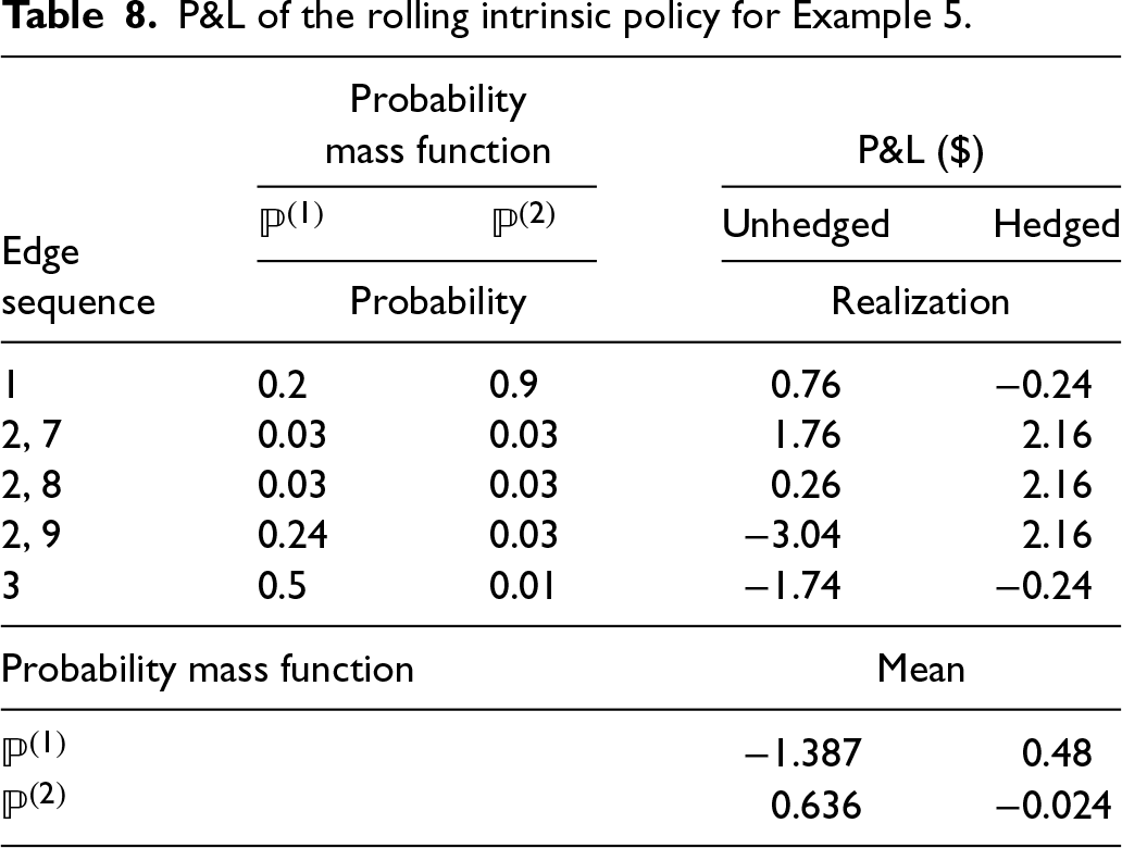
Continuing Examples 1, 2, and 4, suppose that a merchant purchases the storage asset at the no-arbitrage value of the rolling intrinsic policy, $1.24, which is optimal in this case, and monetizes it using this policy. Table 8 reports the resulting P&L realizations for the possible edge sequences in the lattice of Figure 1 along with their likelihoods and means for the probability mass functions
and
, both without and with hedging, that is, forward trading according to this policy. The unhedged P&L varies between −$3.04 and $1.76. It is negative with probability 0.74 and 0.04 and has a mean of −$1.387 and $0.636 for the probability mass functions
and
, respectively. The hedged P&L equals either −$0.24, which by Proposition 1 is the maximal loss one can incur, that is, the difference between the no-arbitrage value of the rolling intrinsic policy and the intrinsic value, or $2.16. For the probability mass functions
and
, the chances that this P&L is negative are 0.7 and 0.91 and its means are $0.48 and −$0.024. Forward trading according to the rolling intrinsic policy shrinks the negative P&L exposure and enhances the positive P&L profile, but can reduce or increase the probability of incurring a P&L loss. On average it turns a large P&L loss into a moderate P&L gain and a modest P&L gain into a small P&L loss for the probability mass functions
and
, respectively.
P&L of the rolling intrinsic policy for Example 5.
P&L of the rolling intrinsic policy for Example 5.
The literature offers some insights into the monetization effectiveness of the rolling intrinsic policy augmented with forward trading in realistic settings. By Proposition 1 the maximal loss of this approach is the difference between the assessed no-arbitrage value of this policy and the intrinsic value of storage. For the natural gas storage settings that de Jong (2015) and Löhndorf and Wozabal (2021) consider this respective loss is about 18% and 21% of the former value on average (the results of de Jong, 2015 here and below pertain to the instances with out of sample parameter estimates; for comparison, the analogous figure is close to 56% for the instances of Example 3). In both cases the average monetization loss is about 3% of the appraised no-arbitrage value of the rolling intrinsic policy. Take as reference the type of forward curve evolution model used by Löhndorf and Wozabal (2021). Secomandi et al. (2015) calibrate to natural gas data both this model and other plausible ones. In their instances the no-arbitrage values of the rolling intrinsic policy that ensue from using the alternative models are on average roughly 2.5% smaller than the analogous values obtained with the reference model. By applying this figure to the results of Löhndorf and Wozabal (2021) that pertain to the rolling intrinsic policy, one can extrapolate that if the other models that Secomandi et al. (2015) examine were used to determine the no-arbitrage value of this policy then on average the corresponding monetization loss would be around 1% of this value (the no-arbitrage values that Löhndorf and Wozabal, 2021 compute, which are analogous to the ones of LMS, are relevant also when markets are incomplete, which is the setting that Secomandi et al., 2015 study).
Forward trading according to the rolling intrinsic policy is not the only way to hedge the P&L of storage assets valued and monetized accordingly. Delta hedging (see, e.g., Hull, 2010: Chapter 6; Luenberger, 2014: Section 12.5) is a common approach based on exact cash flow replication that aims at completely eliminating P&L risk, that is, achieving what is known as a perfect hedge. In other words, in theory the so-hedged P&L equals zero irrespective of the forward curve realizations (in contrast, a merchant would make money for sure provided it secured the storage asset at a price that falls below the no-arbitrage value of the rolling intrinsic policy). In Example 5 the analogue of delta hedging initially sells
Indifference pricing (see, e.g., Smith and Nau, 1995; Carmona, 2009) jointly optimizes the physical trading, operating, and financial trading policies considering risk aversion. Callegaro et al. (2017) and Löhndorf and Wozabal (2021) apply it to electricity swing options and natural gas storage, respectively. In particular, Löhndorf and Wozabal (2021) find that the risk and reward profile of the rolling intrinsic policy differs from the optimal one. If one wishes to use the rolling intrinsic policy to make physical trading and operating decisions, it may be possible to modify these methods so that they take these choices as given and optimize only the financial trades.
Common liquidity concerns (see, e.g., Swindle, 2016; Lassander and Swindle, 2018: Chapter 7) may prevent traders from taking positions in forward contracts for all the maturities that span the term of a storage asset, especially ones with long horizons. The rolling intrinsic policy can be correspondingly adapted by considering bid-ask spreads (Gray and Khandelwal, 2004a), but its performance may degrade. Perfect hedging techniques that indirectly take limited liquidity into account include the ones of Secomandi et al. (2015) and Secomandi and Yang (2022), who apply them to natural gas storage using the rolling intrinsic policy and a least squares Monte Carlo policy, respectively. They report substantial P&L variability reduction compared to no hedging. In particular, the method of Secomandi and Yang (2022), who extend the one of Secomandi (2022), effectively concentrates the hedged P&L around the assessed no-arbitrage value of the asset.
The rolling intrinsic policy is used in practice to manage commodity storage assets on a merchant basis. MNMG emphasize that their partial monetization findings deviate in two substantial ways from what is known about the valuation performance of this policy: (i) The rolling intrinsic policy can perform worse than the intrinsic policy and (ii) it seems to be highly suboptimal. Whereas they ascribe these disparities to informational inconsistency, this paper contends that this argument generally entangles this imprecision with the risk adjustment that distinguishes no-arbitrage valuation. This work argues that at least the first discrepancy arises from the lack of risk adjustment in the MNMG’s study and informational inconsistency is unable to cause the second discordance in approximately 4% of the MNMG’s instances. Further, it shows that the first difference disappears if one executes both the spot and the forward trades of the rolling intrinsic policy, whereas in general doing so does not remove the second dissimilarity. Lastly, it summarizes findings from the literature that suggest that in practical situations this augmented variant of the rolling intrinsic policy yields limited average P&L losses if a storage asset is acquired at the assessed no-arbitrage value of this policy and discusses alternative risk management techniques that may outperform this approach. Additional research could study both the role that risk adjustment may play in the second discrepancy and the impact of forward trading on the expected value of the rolling intrinsic policy and the P&L risk when monetizing commodity storage assets.
MNMG discuss a third discrepancy. They find that in their backtest truncating the ILP horizon can be beneficial for the average value of the resulting rolling intrinsic policy. MNMG state that this observation contradicts what is known about this policy under no-arbitrage valuation (although MNMG cite Cruise et al., 2019, who use deterministic prices and conduct their numerical analysis on data, Nadarajah and Secomandi, 2013 report findings for no-arbitrage valuation consistent with the claimed existing ones; the paper of Nadarajah and Secomandi, 2018 subsumes this work but does not include these results). One may investigate the roles that informational inconsistency and risk adjustment may play in the third disparity.
Generalization error is the loss relative to the optimal objective function value of an MDP, or a valid bound on it, incurred by a policy distinguished by tunable parameters the values of which are estimated with access to a misspecified model of the MDP uncertain data or a sample of such data (see, e.g., Murphy, 2005). MNMG interpret the second discrepancy as evidence that informational inconsistency burdens the rolling intrinsic policy with this error. This view is hard to justify in this setting because this policy does not depend on any adjustable parameters, that is, it works directly on data in a model-free fashion. It would be appropriate if one showed that the rolling intrinsic policy is the output of a calibration process that features risk adjustment (but it would be unclear why such tuning was done with risk adjustment if the goal is to maximize the expected discounted value of this policy without it). More broadly, generalization error is relevant to versions of the rolling intrinsic policy that require calibration, for example ones with truncated horizons (see, e.g., MNMG) or other adjustable parameters (for instance prices in the spirit of the method of Wu et al., 2012, which, however, does not involve tuning; see also work on cost function approximations in reinforcement learning, Powell, 2022: Chapter 13). Further work in this area, also going beyond the rolling intrinsic policy (see, e.g., the technique that MNMG propose), would be valuable.
Footnotes
Acknowledgments
The author thanks Sridhar Seshadri (the department editor), the senior editor, two reviewers, and Selvaprabu Nadarajah for their comments on earlier drafts of this paper.
Declaration of Conflicting Interests
The authors declared no potential conflicts of interest with respect to the research, authorship, and/or publication of this article.
Funding
The authors received no financial support for the research, authorship and/or publication of this article.
How to cite this article
Secomandi N (2024) On the Valuation and Monetization Roles of the Rolling Intrinsic Policy for Merchant Commodity Storage. Production and Operations Management 34(6): 1426–1439.