Sage Journals: Discover world-class research

Abstract

Demand forecasting for seasonal products becomes especially challenging in the case of fast innovations, where the product portfolio is upgraded every season. In addition to the problem of forecasting demand without any historical data, companies also have to deal with frequent stockouts, which bias past sales and provide an unreliable anchor for making new forecasts. We show how one can use machine learning models to leverage information on comparable products from the past together with experts’ forecasts to improve forecasting accuracy. A machine learning forecast using only statistical features results in a forecast error reduction of 24%, measured by weighted mean absolute percentage error, compared to a purely judgmental prediction on data from Canyon Bicycles. Better yet, an integrated human-machine forecast leads to a further 14% reduction in forecast error, indicating that experts’ predictions remain essential for forecasting demand for rapidly innovating seasonal products. The combination of the experts’ knowledge of the future and the machine learning algorithms’ ability to leverage historical information works best in this setting.

Keywords

Judgmental demand forecasting machine learning e-commerce clickstream data Google Trends

1. Introduction

Traditional demand forecasting methods typically rely on historical data. For new products, however, no historical information is available. This is a big challenge companies face in forecasting demand, especially for seasonal products with short life cycles. The demand for highly innovative products driven by the latest technology in the market is even more unpredictable than functional products with long life cycles (Lee, 2002). While product innovation is vital to any company’s sales growth strategy, erroneous forecasts for such products could severely impact the firm. Moreover, companies often face long supplier lead times and therefore have to place orders months before the start of the season. A survey of forecasters by Fildes and Goodwin (2007) shows that most companies make forecasts with a lead time of 3–18 months. In addition, frequent product stockouts during the season give an inaccurate measure of the past demand and therefore provide an unreliable anchor for future forecasts (Jain et al., 2015). Empirical evidence suggests that bias in demand estimation due to the ignorance of stockouts can harm the company’s profitability (Conlon and Mortimer, 2013) and lead to incorrect assumptions about customer preferences toward their products. Furthermore, such stockouts can be attributed to the Key Performance Indicator of zero end-of-period coverage (ECR Australia, 2010).

A common approach to predicting demand for such innovative products is judgmental demand forecasting. Studies show that internal expert judgment is often preferred for new product forecasting (Kahn, 2002; Kahn and Chase, 2018). Experts have access to soft information such as special events, changes in government regulations, competitor’s activities, unforeseen crises, and many more. This type of information is difficult for any statistical model to capture. A survey of practitioners by Fildes and Goodwin (2007) lists the main reasons for using judgment, the most important ones being promotional activities and price changes. An alternative to judgmental demand forecasting is applying machine learning (ML) algorithms to historical data. Since new products do not have any historical data, the data of comparable products from the previous season can be used instead. The sophistication of ML algorithms allows companies to include other types of information, such as clickstream data, in addition to their operational data.

Given these two different forecasting methods, we investigate whether the experts’ judgment is still valuable in the era of big data analytics and advanced ML tools and whether it is beneficial to integrate the two methods. The comparison of the out-of-sample errors from (i) a judgmental forecast, (ii) a ML forecast, and (iii) an integrated human-machine forecast allows us to quantify the value added by expert judgment in improving the demand forecasts. Our results show that an integrated human-machine forecast has the highest accuracy (i.e., 33% weighted mean absolute percentage error (WMAPE) on our example dataset from practice) and therefore is recommended to predict the demand for innovative products in the new season. Additionally, we present a general framework for companies to forecast the demand for the whole selling season several months in advance for a portfolio of innovative products with high demand uncertainty and long supplier lead times in addition to historical data subject to stockouts.

In the next section, we present a review of the literature related to our research. We discuss the integrated forecasting approach for the new season in Section 3, followed by the demand prediction models for the past seasons that serve as important inputs to the new season’s forecasts in Section 4. In Section 5, we present an empirical study using company data. The results of our study are discussed in Section 6, and Section 7 concludes the paper with key insights and potential avenues for future research.

2. Literature Review

Lawrence et al. (2006) provide a comprehensive review of research in the domain of judgmental forecasting. The accuracy of judgmental forecasts is known to increase when the individual forecasts are aggregated, known as the “wisdom of crowds” approach (Ho and Chen, 2007; Cowgill and Zitzewitz, 2015; Bansal and Gutierrez, 2020; Soule et al., 2023). The most notable example of this approach is presented in the Sport Obermeyer case study by Fisher et al. (1994). The authors use the average of the experts’ forecasts to represent the mean of the demand distribution and establish a relationship between demand uncertainty and dispersion among the individual forecasts. These findings are supplemented by Gaur et al. (2007). In addition to previous studies, they find a positive correlation between the variance in demand and the mean forecast. In another study on O’Neill, Cachon and Terwiesch (2013) adjust the new season’s mean demand and estimate demand uncertainty using the previous season’s A/F ratios (actual/demand forecast). They eliminate systematic bias in the forecasts by multiplying the new mean forecast with the average of the last season’s A/F ratio. Furthermore, demand uncertainty is obtained by multiplying the standard deviation of the past A/F ratios with the current season’s mean forecast. Diermann and Huchzermeier (2016a, 2016b, 2017) apply this methodology of A/F ratios in their application on Canyon Bicycles’ data. In addition, they identify at which level of aggregation of products should the A/F ratios be calculated to adjust the bias of expert forecasts in order to avoid both over-fitting and over-aggregation.

Researchers agree that a combination of judgmental and quantitative forecasts performs better than the individual forecasting methods (Blattberg and Hoch, 1990; Goodwin, 2002; Sanders and Ritzman, 2004). Sanders and Ritzman (2004) categorize the integration methodologies into four types: (i) Judgmental adjustment of the quantitative forecast, (ii) quantitative correction of the judgmental forecast, (iii) combining judgmental and quantitative forecast, for example, using a weighted average, and (iv) judgment as an input to model building. Blattberg and Hoch (1990) show that a 50% model + 50% human approach outperforms either of the individual methods. Goodwin (2002) reviews the effectiveness of different integration methods in improving short-term forecasts. Fildes et al. (2009) analyze the effectiveness of different expert adjustment procedures on improving forecast accuracy. Trapero et al. (2013) examine the accuracy of judgmental adjustments to sales forecasts in the presence of promotions and find that experts still add value to their model. Seifert et al. (2015) study the impact of contextual and historical anchors for expert forecasts through a field experiment in the music industry. They analyze the conditions under which contextual and historical information should be provided to the forecasters and show that restricting the information to contextual anchors is better when judgmental forecasts are integrated with statistical methods. A recent literature review by Arvan et al. (2019) reveals that the majority of the papers in this domain focus on lab experiments, with only 15% of the papers showcasing a real-world setting in the form of case studies and field experiments. Furthermore, the literature presents contrasting findings regarding the value added by experts (see, e.g., Griffin and Brenner, 2004). Our paper adds to the empirical literature with a numerical analysis of company data investigating whether experts play a critical role in the company’s demand forecasting process.

New product forecasting methods based on leveraging comparable product information serve as an alternative to judgmental demand forecasting. This area has gained increasing attention in recent years with a focus on data-driven models. The availability of big data allows e-commerce firms to gain meaningful insights from their customer’s browsing behavior in addition to Point-of-Sales data (Fisher and Raman, 2018; Aouad et al., 2019). ML models are becoming increasingly popular for demand forecasting as they are more accurate at making predictions on high-dimensional datasets by overcoming the shortcomings of traditional linear regression models. Ferreira et al. (2016) apply regression trees to predict the demand for new styles sold in flash sales for an online fashion retailer. Baardman et al. (2018) develop an algorithm that combines clustering and penalized linear regression for forecasting the demand for new products and benchmark their model against several widely used forecasting methods on two retailer datasets. Hu et al. (2019) present an empirical analysis using clustering methods to forecast life cycle curves for new products that are similar to past launches. However, current literature applications are limited to time series predictions and/or short-term forecasts. In contrast, in our study, we derive a point forecast for the complete season before the season begins, a common approach used by companies selling products with short life cycles and long lead times (Fisher and Raman, 1996; Cachon and Terwiesch, 2013). Another popular approach for new product forecasting is the application of diffusion models. However, our study does not consider them as they are best suited for new-to-the-world technologies and not product improvements (Kahn, 2002).

Our work lies at the intersection of literature related to judgmental forecasting and data-driven models. Previous research on judgmental forecasting is limited to basic statistical models, and the incorporation of ML algorithms in this area has not yet been explored. Our paper aims to expand the literature on empirical studies in this area by exploring the potential advantages of combining the strengths of the two streams for forecasting demand for rapidly innovating products.

3. The Integrated Demand Forecast for the New Season $τ + 1$

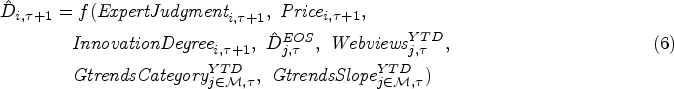
Our objective is to evaluate the value of integrating the experts’ judgment with statistical features in a machine learning model to forecast the demand ${\hat{D}}_{i, τ + 1}$ for product $i$ in the new season $τ + 1$ . We formulate this as a general supervised learning problem, as shown in Equation 1 (All model notations can be found in Table A2 in the Appendix.) The function $f (.)$ can take various forms, depending on the ML model applied.

\begin{aligned} {\hat{D}}_{i, τ + 1} & = f ({ExpertJudgment}_{i, τ + 1}, \\ {NewProductStatisticalFeatures}_{i, τ + 1}, \\ {PastProductStatisticalFeatures}_{j, τ}) \end{aligned}

(1)

E x p e r t J u d g m e n t_{i, τ + 1}

refers to the mean of the expert forecasts for the new product

i

in the new season

τ + 1

N e w P r o d u c t S t a t i s t i c a l F e a t u r e s_{i, τ + 1}

represents statistical features for the new season

τ + 1

that are already known at the time of forecasting, such as the price of the new product. Additionally,

P a s t P r o d u c t S t a t i s t i c a l F e a t u r e s_{j, τ}

constitutes statistical features of product

j

in the current season

τ

. Product

j

is comparable in features to the new product

i

. This can include operational features such as the sales history of comparable products, online data such as web traffic and Google Trends data, and market and competitor data, to name a few.

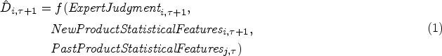
To forecast the demand for products in the new season using Equation 1 and to assess the weights given to the experts and the statistical features, we evaluate the following ML regression models: (1) ordinary least squares (OLS) regression, (2) penalized regression—Lasso and Ridge, (3) Random forests, and (4) Extreme Gradient Boosting. The OLS regression is the simplest form of regression and, therefore, commonly applied for simple prediction tasks. However, this method relies on many assumptions that are often not met in practical applications. For example, the presence of collinearity amongst the variables can result in inaccurate estimates of the regression coefficients. The drawbacks of the OLS regression can be overcome by using penalized regression that allows shrinkage (or regularization) of the model coefficients to reduce variance at the cost of slightly higher bias. This can prevent the model from over-fitting on the training data and lead to more accurate predictions on new data. The first type of penalized regression, the Ridge regression, is a variation of the OLS regression with an additional penalty term in the loss function, given by $R S S + λ \sum_{l = 1}^{p} β_{l}^{2}$ , where $R S S$ is the residual sum of squares (i.e., the OLS loss function) and $β_{l}$ denotes the coefficients of the $l = 1, \dots, p$ parameters in the model. The tuning parameter $λ$ shrinks the coefficients $β_{l}$ toward zero (but never equal to zero). The second type of penalized regression, the Lasso regression, shrinks some of the coefficients to zero and can therefore perform variable selection. This is advantageous in problems with a large number of features. The loss function for the Lasso regression is given by $R S S + λ \sum_{l = 1}^{p} | β_{l} |$ . Both types of penalized regression provide the advantage of reduced over-fitting compared to the OLS model and can also handle multicollinearity within the dataset.

We also analyze tree-based ensemble methods, Random Forests, and Extreme Gradient Boosting, that combine the predictions from multiple decision trees. Tree-based models split the predictor space into regions and derive outcomes based on the mean values of these regions in case of a regression problem. These models are easy to interpret and can identify the most important predictor variables. However, the intuitiveness is reduced when aggregation such as Random Forests is applied, although they substantially improve accuracy over a single decision tree. Hastie et al. (2009) provide a detailed description of all the models discussed here. We can also apply Neural Networks to regression problems. However, we do not include this method in this study as it is better suited for very large datasets. Moreover, it is a “black-box” approach, which makes it difficult to interpret the model mechanism, especially in our context where we wish to identify the significance of judgmental forecasts. Each of the aforementioned ML algorithms has advantages and disadvantages, and there is no single “best” model. The best-performing model varies based on the problem at hand. Therefore, we compare different methods on our empirical dataset, both in terms of accuracy and complexity, to arrive at the most suitable model for our setting.

To check how well the ML models are able to forecast the demand for the new season, we compare the demand forecasts ${\hat{D}}_{i, τ + 1}$ with the “true” demand $D_{i, τ + 1}$ for product $i$ in that season. For a given product category $M$ with no stockouts in a given season, the demand for all products $i \in M$ is equal to the observed sales ( $D_{i} = S_{i}$ ). However, in the presence of stockouts in any of the products in product category $M$ , substitution among the products may occur. Hence, on the one hand, the demand for the out-of-stock product may be underestimated ( $D_{i} \geq S_{i}$ ). On the other hand, the demand for a possible substitute product may be overestimated ( $D_{i} \leq S_{i}$ ). The true demand for a product with stockouts is the estimated demand potential during the periods with stockouts, in addition to the observed sales $S_{i}$ . It is calculated ex-post, i.e., after the selling season is over (for more details, see Section 4.1).

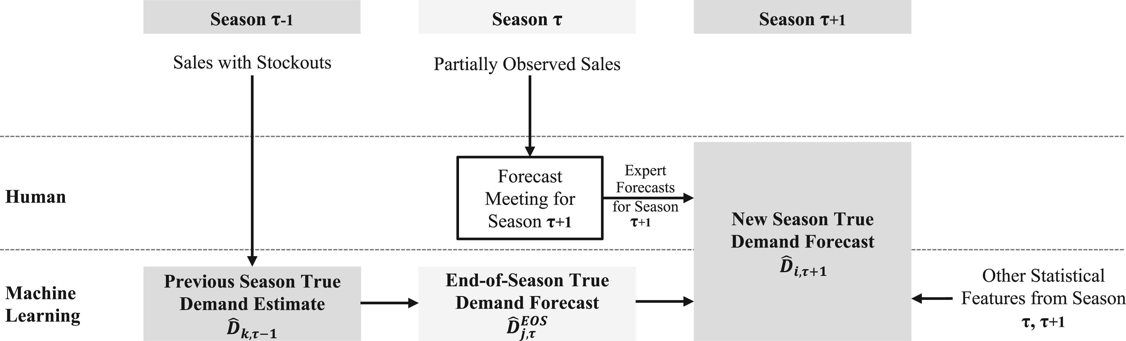
Figure 1 illustrates the demand forecasting process over three seasons. The forecast for product $i$ in the new season $τ + 1$ is developed in season $τ$ . At this point in time, we have data on product $k$ from the previous season $τ - 1$ and on product $j$ from the first half of the current season $τ$ . Product $j$ from the current season is comparable to product $i$ of the new season and product $k$ of the previous season is comparable to product $j$ of the current season. We first calculate the true demand for comparable products $k$ and $j$ from the seasons $τ - 1$ and $τ$ before forecasting the demand for new product $i$ in season $τ + 1$ . The figure highlights how human judgment and ML elements are combined to develop the integrated demand forecasts for season $τ + 1$ .

Figure 1.

Overview of the demand forecasting process over three seasons.

4. Estimation of True Demand in the Past Seasons

τ - 1

and

τ

The true demand models for seasons $τ - 1$ and $τ$ estimate the demand potential during weeks of stockouts in the past season $τ - 1$ , and the demand for the remaining weeks of the current season $τ$ . The key difference between the development of the two true demand prediction models stems from the type of data available to estimate the demand. To calculate the true demand in the previous season $τ - 1$ , complete data is available over all weeks since the season is over (for example, web traffic data), whereas for the current season $τ$ , only partial data is available since the season is not yet over. Therefore, we use two different formulations for calculating the demand for these two seasons. As shown in Figure 1, the true demand estimates from the previous and current seasons are important in forecasting the new season’s demand.

4.1. Estimation of True Demand during Stockouts (previous season $τ - 1$ )

Several studies in revenue management have shown applications of discrete choice models for demand estimation under stockouts (see Ratliff et al., 2008). Some of these approaches need specific information, such as the exact time of customer arrivals (Kök and Fisher, 2007) or market share estimates (Vulcano et al., 2012; Abdallah and Vulcano, 2021). This type of information is often imprecise or not available to the company, for example, due to market expansion or contraction. In contrast, we show the application of ML models using data that is easily available at most companies, for example, web traffic data, to calculate the true demand estimate.

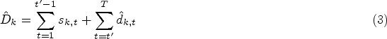
For a given product category $M$ , we first identify the week $t^{'}$ when product $k$ (a previous season product comparable to product $j$ of the current season) starts to stock out. We truncate the sales curve $S_{k}$ for all $k \in M$ at this week $t = t^{'}$ and estimate the true demand ${\hat{D}}_{k}$ from week $t^{'}$ when stockouts occur using $P r o d u c t F e a t u r e s_{k, t}$ available for product $k$ in week $t$ , as shown in Equations 2 and 3. These product features can be selected based on the company’s application. Some examples of such features that can be used in estimating the true demand of the product include the average number of website views for product $k$ in week $t$ or the interest in online search using Google Trends for the product $k$ in week $t$ . The reason for considering all products in the category and not only the out-of-stock products is to account for possible substitution behavior (refer to the E-Companion section EC.1.1 for substitution behavior analysis).

{\hat{d}}_{k, t} = \dot{f} (P r o d u c t F e a t u r e s_{k, t})

(2)

The true demand

{\hat{D}}_{k}

for product

k

can be calculated by summing over the weekly sales

s_{k, t}

or the observed demand until the point of stockout

t = t^{'}

and the estimated demand potential

{\hat{d}}_{k, t}

(from Equation 2) for the remaining weeks till the end of the season

t = T

{\hat{D}}_{k} = \sum_{t = 1}^{t^{'} - 1} s_{k, t} + \sum_{t = t^{'}}^{T} {\hat{d}}_{k, t}

(3)

4.2. End-of-season True Demand Prediction (current season

τ

)

As illustrated in Figure 1, we also forecast the true demand ${\hat{D}}_{j, τ}^{E O S}$ for product $j$ in the current season $τ$ using data available until the point of forecast. This provides an estimate of how many products will be sold in total by the end of the current season and can be used in production and promotion planning before the current season ends. We also show that the total end-of-season demand prediction can be an important predictor for the new season’s demand forecast in our empirical study in Section 5.

We can add the current season’s true demand prediction as a feature in the new season’s demand forecasting model. This allows us to include the most up-to-date information in our ML model.

The end-of-season true demand estimate ${\hat{D}}_{j, τ}^{E O S}$ for product $j$ in the current season $τ$ can be estimated if we know the trajectory of that product’s demand curve. We assume that this trajectory remains consistent from one season to another and therefore we can use the trajectory of the demand curves from the previous season $τ - 1$ to estimate the end-of-season true demand in the current season $τ$ . The trajectory of the demand curve for each product $k$ in the previous season $τ - 1$ is obtained from the total normalized true demand ${\tilde{d}}_{k, m}$ for product $k$ until week $m$ , as shown in Equation 4.

{\tilde{d}}_{k, m} = \frac{\sum_{t = 1}^{m} d_{k, t}}{D_{k}}, 1 \leq m \leq T

(4)

where

D_{k}

is the total true demand for product

k

for the complete season.

D_{k} = S_{k}

(where

S_{k}

is the total observed sales for product

k

) if there are no stockouts, and

D_{k} = {\hat{D}}_{k}

(where

{\hat{D}}_{k}

is the total true demand for product

k

as calculated in Equation 3) if there are stockouts.

{\hat{d}}_{k, t}

is the demand for product

k

in week

t

of the season (

d_{k, t} = s_{k, t}

if there are no stockouts, and

d_{k} = {\hat{d}}_{k}

if there are stockouts).

The products from the previous season $τ - 1$ are clustered by applying unsupervised learning algorithms to these trajectories of demand curves. In the next step, we determine the cluster $c$ to which the products from the current season $τ$ belong using only its initial data until the observed week $m < T$ . This is a multiclass classification problem. Therefore, we apply different ML classification algorithms to assign the products to the different clusters. We can then use the mean value of the cluster members to predict the total demand for the current season, as shown in Equation 5.

{\hat{D}}_{j, τ}^{E O S} = \frac{\sum_{t = 1}^{m} d_{j, t, τ}}{\frac{\sum_{k = 1}^{n_{c}} {\tilde{d}}_{k, m, τ - 1}}{n_{c}}}

(5)

where

\sum_{t = 1}^{m} d_{j, t, τ}

is the cumulative demand for product

j

until week

m

of season

τ

, i.e., until the most recent week of available data in the current season.

\sum_{k = 1}^{n_{c}} {\tilde{d}}_{k, m, τ - 1} / n_{c}

is the mean proportion of fulfilled demand for products,

k = 1, \dots, n_{c}

in cluster

c

(where

n_{c}

is the number of products in cluster

c

) by week

m

in the previous season

τ - 1

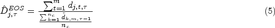
For example, if a product has a demand of 650 units in the first 6 months of the season with approximately 25 units sold each week. In that case, we can classify the product in one of the clusters using a multiclass classification algorithm that has been trained on the demand clusters of all products in the previous season. If for this assigned cluster, 49% of the total season’s demand is fulfilled in the first 6 months, then from Equation 5 we can estimate the total end-of-season true demand for the product as 1,327 units (i.e., $650 / 49 %$ ). Similarly, we can predict the total end-of-season true demand for every product during the season on a rolling basis based on the weeks of sales observed.

5. Empirical Study

We look at companies that grow fast. Fast growth indicates innovation making it difficult to predict demand in a turbulent market. We use data from one such firm, Canyon Bicycles, a German direct-to-consumer brand for premium bicycles, to predict the demand for their bikes in the new season and to quantify the contribution of the company’s experts to the forecasting accuracy. As part of the research, we got direct access to Canyon Bicycles’ data with cooperation from the Business Intelligence team. The company operates in a fiercely competitive innovation-driven market with high demand uncertainty and has exhibited exponential revenue growth in the last five years (see Figure 2). Figure 3 illustrates the current product tree at the company. At the top-most level, the bikes are categorized into Road, Mountain, Gravity (downhill bikes), and Urban/Fitness. As we go down the product hierarchy, the bikes are further classified by function into bike families, the material of the frame, platform, gender, and finally, at the SKU level by size and color. Five years ago, only a “pruned” version of the current product tree existed with just two categories—Road bike and MTB and up to level 3 in the given figure (Diermann and Huchzermeier, 2017). Since then, the number of bikes has nearly doubled, with new bike designs, catering to the latest customer preferences being added to the product portfolio. Furthermore, forecasts are made at a very disaggregated level (i.e., at the Product Group level, as shown in Figure 3), adding further complexity to the forecasting task.

Figure 2.

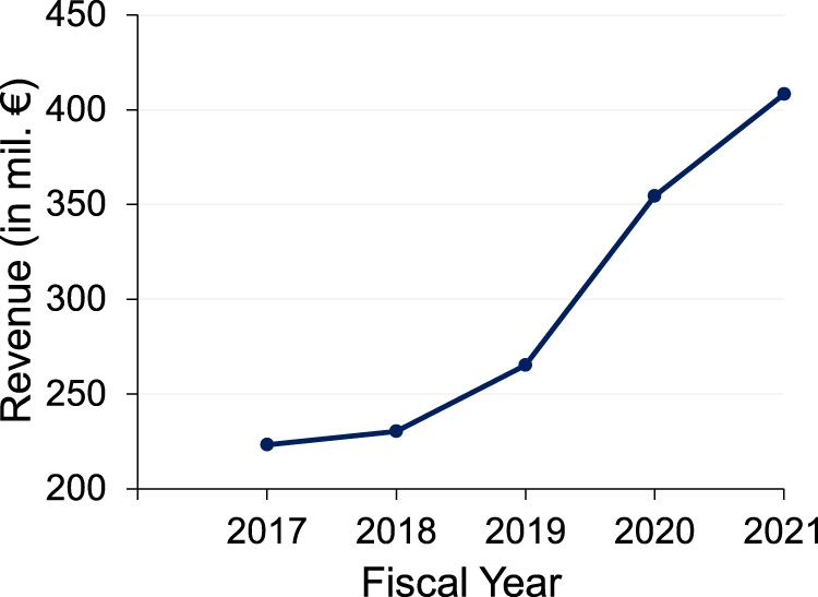
Revenue growth of Canyon Bicycles over the last five years.

Figure 3.

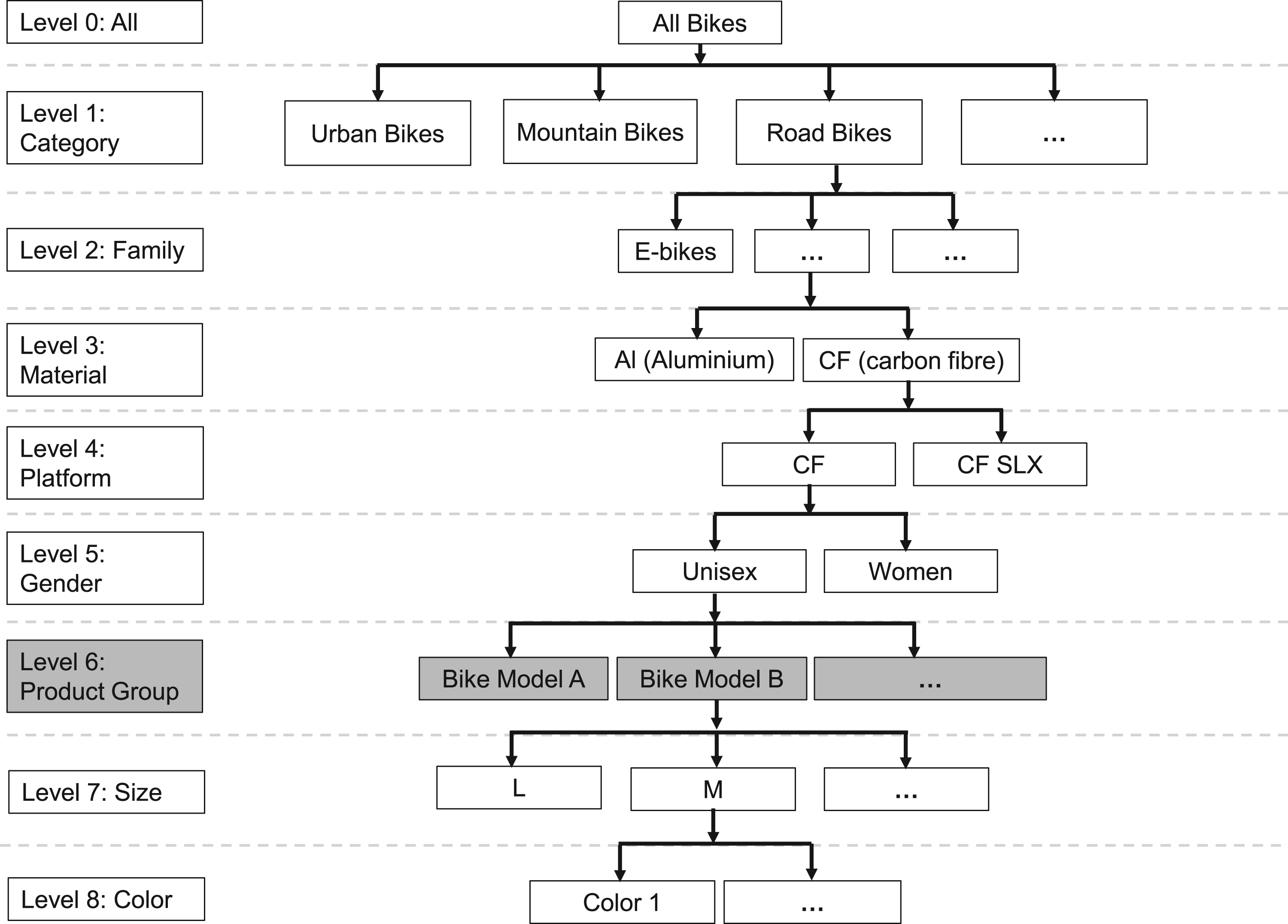
Current product tree at Canyon Bicycles.

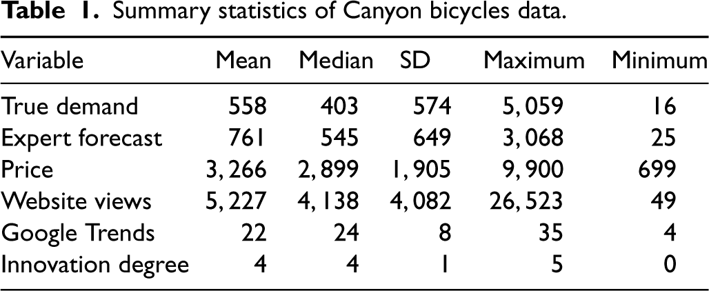
We collected data from 2017 to 2020 for Road bike and MTB. Road bike and MTB collectively account for 74% of the company’s revenue. Every season has close to 100 bike models and more than 40,000 bikes are sold each season. Some summary statistics of the data are presented in Table 1. The selling season at Canyon Bicycles starts in October and ends in September of the following year¹ and consists of 52 weeks. All operational data, such as sales, promotions, and company forecasts, are available at the bike model or Product Group level, aggregated on all sizes and colors (see Figure 3). Sales data in the form of order entries before cancelations were taken as this provides a true indication of the demand.

For every bike model, we also have information on comparable bikes from the previous seasons, including the degree of innovation. The degree of innovation measures how innovative the new product is on a scale from 0 to 5, where 0 implies no change in the product features from the previous season, whereas 5 indicates a completely new development. Figure 4 shows that around 90% of the products, on average, are upgraded every season, out of which approximately 31% are completely new developments (innovation degree of 5), 60% are specification changes, e.g., modified bike components such as brakes (innovation degree between 3 and 4), 2% are artwork changes (innovation degree of 2), and the remaining are carry over bikes with no changes or minor changes only in the packaging (innovation degree between 0 and 1).

Additionally, we collected online data from Google Analytics, such as product views on the website. We also extracted Google Trends data which is publicly available. We retrieved this data for all the bike families since the bike model level was too granular to return any results. Furthermore, we obtained data on the coronavirus disease 2019 (COVID-19) pandemic, which is freely accessible at https://ourworldindata.org/coronavirusourworldindata.org (see Ritchie et al., 2020). We also obtained approximate market shares for all bike families. A brief description of the dataset can be found in Table A1 in the Appendix.

Most of Canyon Bicycles’ bike parts suppliers are located in Asia and require capacity reservations in advance. Therefore, the demand forecast for the complete season needs to be finalized several months before the start of sales to ensure sufficient product availability (Note that for this reason, the push-pull supply chain segmentation approach recommended by Simchi-Levi and Timmermans (2021) is not an option in our case.) Furthermore, we need to account for the demand potential during stockouts in the previous season when forecasting demand for the new season (see Figure 5).

5.1. New Season True Demand Forecast

Based on the data collected from Canyon Bicycles, the following features are included in the demand forecasting model shown in Equation 1. This set of features aligns with our application’s needs but can be tailored to specific requirements of the company.

\begin{aligned} {\hat{D}}_{i, τ + 1} & = f ({ExpertJudgment}_{i, τ + 1}, {Price}_{i, τ + 1}, \\ {InnovationDegree}_{i, τ + 1}, {\hat{D}}_{j, τ}^{E O S}, {Webviews}_{j, τ}^{Y T D}, \\ {GtrendsCategory}_{j \in M, τ}^{Y T D}, {GtrendsSlope}_{j \in M, τ}^{Y T D}) \end{aligned}

(6)

E x p e r t J u d g m e n t_{i, τ + 1}

represents the expert forecasts for product

i

in the new season

τ + 1

P r i c e_{i, τ + 1}

and

I n n o v a t i o n D e g r e e_{i, τ + 1}

are

N e w P r o d u c t S t a t i s t i c a l F e a t u r e s_{i, τ + 1}

from Equation 1.

P r i c e_{i, τ + 1}

indicates the price of product

i

in the new season

τ + 1

, and

I n n o v a t i o n D e g r e e_{i, τ + 1}

is the degree of innovation of the new product

i

from the previous version of the product in the current season.

{\hat{D}}_{j, τ}^{E O S}

W e b v i e w s_{j, τ}^{Y T D}

G t r e n d s C a t e g o r y_{j \in M, τ}^{Y T D}

and

G t r e n d s S l o p e_{j \in M, τ}^{Y T D}

are

P a s t P r o d u c t S t a t i s t i c a l F e a t u r e s_{j, τ}

from Equation 1.

{\hat{D}}_{j, τ}^{E O S}

represents the true demand for product

j

, that is comparable to the new product

i

, at the end of the current season

τ

W e b v i e w s_{j, τ}^{Y T D}

represents the average website views for product

j

till the date of forecasting in the current season

τ

. The equation further includes two features based on the Google Trends data for every product

j

in the product category

M

in the current season

τ

, given by

\begin{aligned} {GtrendsCategory}_{j \in M, τ}^{Y T D} & = \frac{G t r e n d s C o m p a n y_{M, τ}^{Y T D}}{G t r e n d s C a t e g o r y_{M, τ}^{Y T D}} \end{aligned}

(7)

\begin{aligned} {GtrendsSlope}_{j \in M, τ}^{Y T D} & = | \frac{Δ G t r e n d s C o m p a n y_{M, τ}^{Y T D}}{Δ G t r e n d s C a t e g o r y_{M, τ}^{Y T D}} | \end{aligned}

(8)

Table 1.

Summary statistics of Canyon bicycles data.

Variable	Mean	Median	SD	Maximum	Minimum
True demand	558	403	574	5,059	16
Expert forecast	761	545	649	3,068	25
Price	3,266	2,899	1,905	9,900	699
Website views	5,227	4,138	4,082	26,523	49
Google Trends	22	24	8	35	4
Innovation degree	4	4	1	5	0

Google Trends indicates the popularity of keywords on Google search on a scale of 1 to 100 based on search volume. Equation 7 represents the ratio of average interest on Google Trends for the company product category to the overall product category. Equation 8 depicts the absolute ratio of the change in Google Trends within the season for the company product category to the change in Google Trends for the overall product category. These features allow us to capture the relative interest for the companies’ products to the general interest in different product categories based on internet search volume.

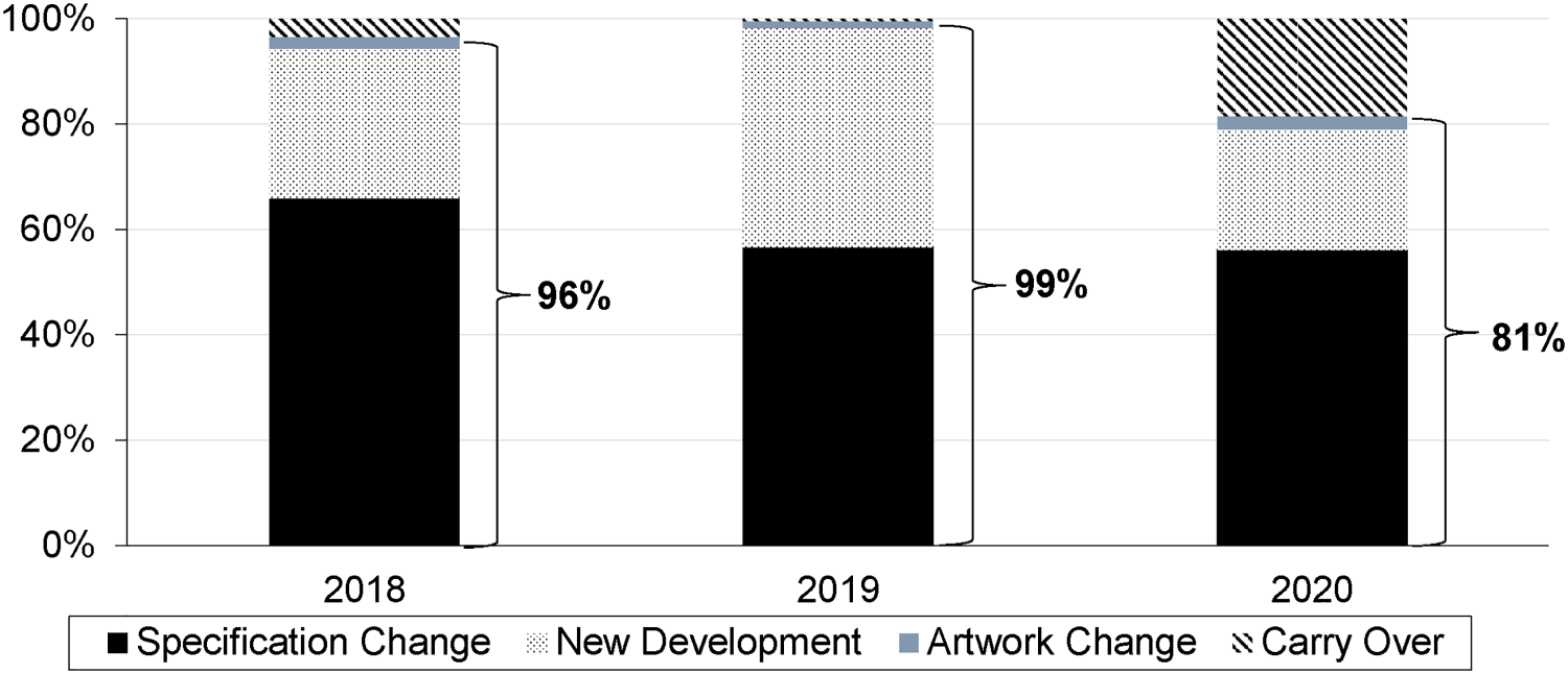
Following the direction of our research question, we wish to evaluate the value of adding expert forecasts ( $E x p e r t J u d g m e n t_{i, τ + 1}$ ) to our model. A team of experts within the company convenes to make a forecast three times before a new season begins. The first meeting takes place one year before the season, the next meeting takes place half a year before the season, and the final meeting happens a month before the season. These meetings are internally referred to as “Obermeyer” meetings after the famous Sport Obermeyer case study by Fisher et al. (1994). The aim of these meetings is to gather experts from marketing, sales, finance, design and production, including the top management, to discuss the strategy for the new season. Country managers from abroad also join the meetings to provide insights from their respective markets.

Figure 4.

Percentage of bike models in the different product innovation categories at Canyon Bicycles.

Figure 5.

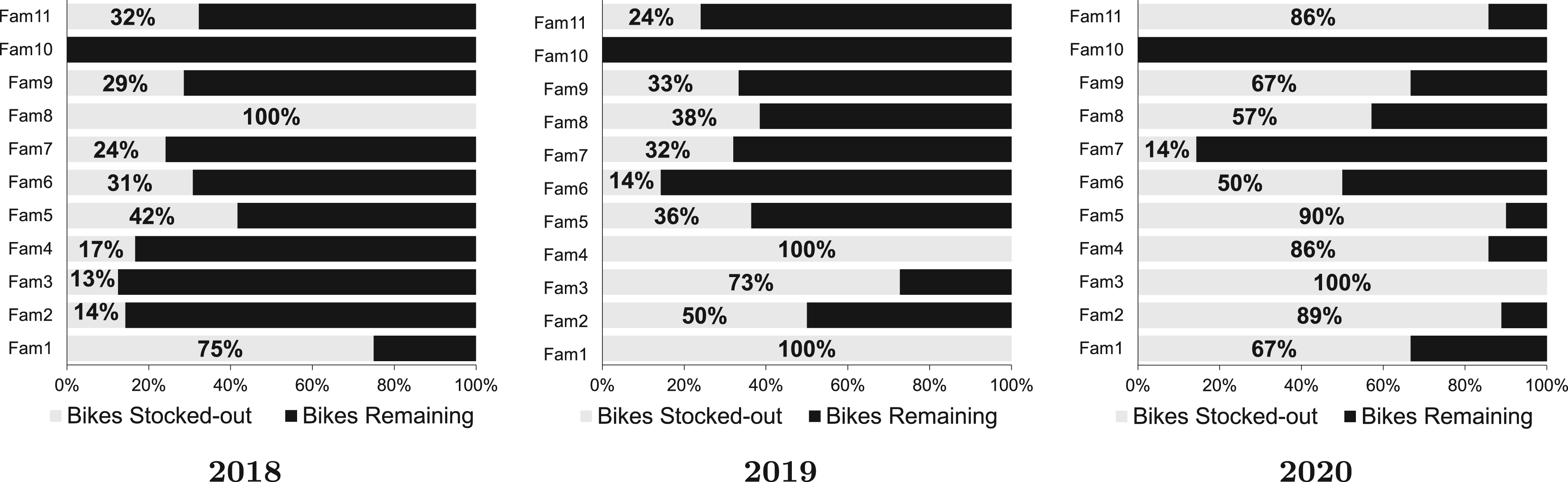
Percentage of bike models in a bike family that stocked out by the end of the season.

Typically, a meeting begins with a review of the past sales season, followed by the introduction of the new season’s product line-up. The category and brand managers describe the new bike designs and their positioning in the market. All presentations follow a standard format to provide the same information across all products to the forecasters. Once the experts have all the information, they individually derive an estimate of the demand for every bike in the upcoming season. After the meeting, the average of the individual forecasts is calculated and treated as the final demand forecast. These forecasts are used as inputs for ordering decisions and production planning. Although all three meetings occur before the start of the new season, the second forecast meeting, which takes place around 6 months before the beginning of the season, is regarded as the most crucial one. This is because 80% of the orders are firmly placed by this date, after which there is only 20% room for any changes in the order quantities. Furthermore, any orders placed after this period risk a delay in availability as bike components can be expected to arrive only after half of the new season is over due to long lead times at the supply end. Therefore, we center our study around the expert forecasts obtained from the second meeting.

Mr. Roman Arnold, the co-founder and former CEO of Canyon Bicycles, realized early on the gap between the expert forecasts and demand and adjusted the aggregate bike forecasts by a constant factor each year. A case study by Diermann and Huchzermeier (2017) built upon this approach by searching for the optimal aggregation level of the bikes to apply the bias correction based on past ratios of actual versus forecasted demand (A/F ratios). However, this method is unsuitable when the bias changes over time (Goodwin, 1997). Additionally, as category managers change from time to time and team sizes shrink due to product proliferation, these A/F ratios can become less stable from one season to another. Further analysis of the A/F ratios at varying levels of the product hierarchy and model results can be found in the E-Companion section EC.3.

We use the observed sales until the most recent week in the current season $τ$ to predict the current season’s true demand ${\hat{D}}_{j, τ}^{E O S}$ to include as a feature in our model. Our results show that including this term leads to more accurate forecasts as compared to including only observed sales from the initial weeks of the current season in the model. Using the methodology from Section 4.1 we first calculate the true demand ${\hat{D}}_{k}$ for all bikes in the previous season $τ - 1$ (the true demand calculation for our particular dataset using web traffic and other features can be found in the E-Companion section EC.1.2 and then cluster the bikes based on the trajectory of their normalized true demand curves as shown in Section 4.2. On applying the clustering algorithms on the normalized true demand curves of all bikes from 2017 to 2019, we find that three distinct shapes of demand curves emerge every year (as shown in Figure 6). The first cluster represents an S-shaped demand curve for bikes with a consistent demand throughout the season with little fluctuations. The majority of bikes fall under this cluster. The second cluster represents an inverted U-shaped demand curve and comprises bikes that start with a high demand that gradually decreases by the end of the season. Some of these bikes are new product launches, generating consumer interest in the initial weeks. Some bikes in this cluster are also released later in the season, close to New Year, and therefore have higher sales in the beginning. The last cluster represents a J-shaped demand curve and includes bikes that experience higher demand in the second half of the season. Most of these bikes are “classic” Road and Triathlon bikes that have increased demand during spring/summer. For further details on the clustering algorithms applied and metrics for the optimal number of clusters selection, refer to the E-Companion section EC.2.1. Then from Equation 5 we can estimate the total end-of-season true demand ${\hat{D}}_{j, τ}^{E O S}$ for all bikes in the current season $τ$ for our forecasting model. E-Companion sections EC.1.5 and EC.2.2 compare the accuracy of different ML models on out-of-sample data for the previous season and current season true demand prediction models.

Figure 6.

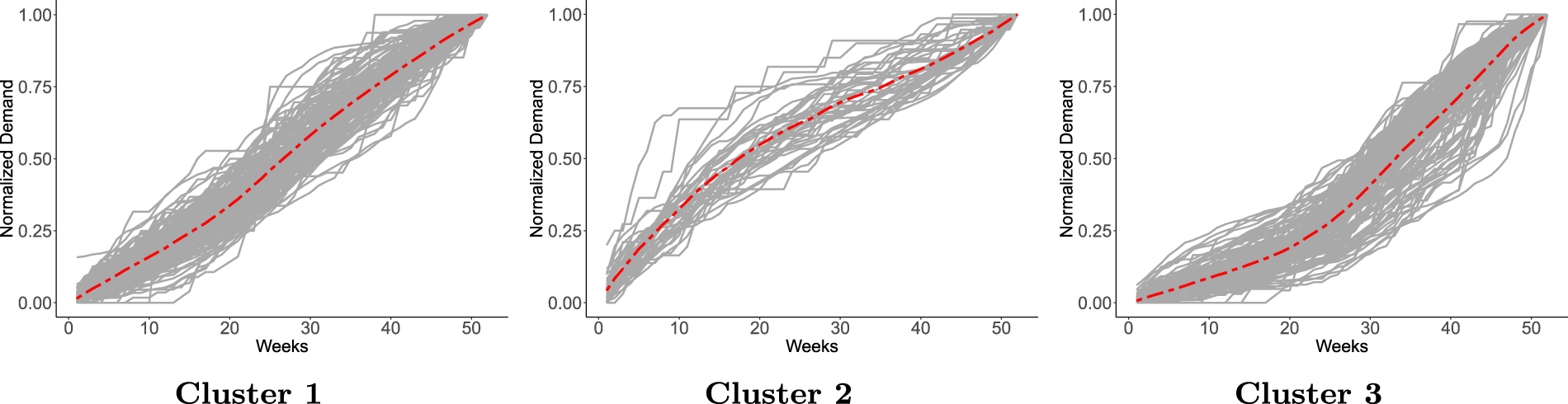
Clusters based on true demand curves for all bike models from 2017 to 2019.

5.2. Training and Testing Procedure

We develop forecasts for the new season $τ + 1$ half a year before the start of the season, as shown in Figure 1. This means we have 6 months of data from the current season $τ$ and a full year of data from the previous season $τ - 1$ . We need historical data on comparable bikes from the past for our demand forecasting model. We find that using data from two years ago significantly reduces the size of our training data as fewer comparable products for the new product are available as the product portfolio is rapidly changing every season. Therefore, we use a combination of observed sales till the forecast meeting and demand forecasts for the second half of the current season to train our ML model with the most recent information. We find that this method results in more accurate forecasts than using only the previous season’s complete demand to train the model.

We apply log transformation to both the independent and dependent variables in Equation 1. This formulation is common in demand forecasting (Cohen et al., 2017; Wolters and Huchzermeier, 2021). It allows us to model non-linear relationships; more specifically, we can analyze the elasticity between two variables, such as demand and price. To obtain the final demand forecasts in the original scale, we re-transform the log values of demand using the Duan smearing estimate (see Duan, 1983). This correction factor overcomes the problem of re-transformation bias by multiplying the final predictions with $\frac{1}{n} \sum_{i = 1}^{n} \exp (E r r o r_{i, τ + 1})$ where $E r r o r_{i, τ + 1}$ refers to the residuals from the regression. The smearing estimate is calculated by averaging the exponential of the residuals over all products $i = 1, \dots, n$ (where n is the total number of products) in the dataset.

We also apply a 10-fold cross-validation on the training data for parameter tuning and to avoid over-fitting (Hastie et al., 2009; Hyndman and Athanasopoulos, 2018). A 10-fold cross-validation randomly splits the dataset into 10 equally sized subsets. The algorithm is then trained on 9 subsets, and the remaining subset is used as the hold-out sample to test the model’s accuracy. This process is repeated 10 times, and the performance over all hold-out samples is averaged to obtain the cross-validation error for that algorithm. The model parameters that give the best performance during cross-validation are chosen to develop predictions for the test dataset. Cross-validation also ensures that the model is exposed to different subsets of data in order to avoid over-fitting to the training data.

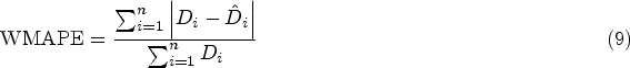
We use WMAPE as our metric for training the models and to measure the model’s performance on test data. WMAPE is a variation of the mean absolute percentage error (MAPE). MAPE is one of the most commonly used metrics for measuring forecasting accuracy as it is scale-independent and interpretable. Although MAPE has many advantages, it also has the disadvantage of excessively enlarging errors for small sales units. For datasets with a vast range of sales volumes, relying on MAPE as a measure of accuracy can be misleading. Therefore, we calculate the WMAPE by weighing the MAPE on sales volume, as shown in Equation 9.

WMAPE = \frac{\sum_{i = 1}^{n} | D_{i} - {\hat{D}}_{i} |}{\sum_{i = 1}^{n} D_{i}}

(9)

where

{\hat{D}}_{i}

is the forecasted demand for product

i

and

D_{i}

is the true demand for product

i

\sum_{i = 1}^{n} D_{i}

is the sum of true demand over products

i = 1, \dots n

As an example, we illustrate the steps to test the accuracy of the demand forecasts for 2019 after training the model on data from 2017 and 2018, as shown below.

(1)

True demand estimation in the presence of stockouts for 2017: ${\hat{D}}_{k, 2017}$

Input: Observed sales, product availability, price and discount, and online data² from 2017

Output: True demand for the weeks with stockouts in 2017 (I)

Pre-process the data to identify weeks with stockouts and discounts

(II)

Handle discount peaks to obtain base demand from sales if needed (see E-Companion section EC.1.3)

(III)

Truncate the sales curve at the week of stockout to train the ML model (with cross-validation) on weekly online data (or other features) (see Equation 2 and E-Companion section EC.1.2)

(IV)

Predict the true demand for periods with stockouts using the trained ML model

(V)

The observed sales until the point of stockout plus the predicted demand after the point of stockout gives us the true demand for 2017, ${\hat{D}}_{k, 2017}$ (see Equation 3)

(2)

End-of-season true demand forecast for 2018: ${\hat{D}}_{j, 2018}^{E O S}$

Input: ${\hat{D}}_{k, 2017}$ (from Part 5.2.), first half of observed sales in 2018

Output: Rolling demand forecast for the remaining season in 2018 (I)

Apply unsupervised learning algorithms to cluster the true demand curves from 2017 and choose the optimum number of clusters (see E-Companion section EC.2.1)

(II)

Train a multiclass classification model (with cross-validation) on the true demand curves from 2017 based on the generated cluster labels

(III)

Apply the classification model on sales data from the first half of 2018 to assign the product to one of the clusters

(IV)

Forecast the demand for the remaining weeks of 2018 based on the mean demand trajectory of the particular cluster (see Equation 5)

(V)

The sales from the first half of the season plus the predicted demand from the second half of the season gives us the end-of-season true demand estimate for 2018, ${\hat{D}}_{j, 2018}^{E O S}$

(3)

New season true demand forecast for 2019: ${\hat{D}}_{i, 2019}$

Input: ${\hat{D}}_{j, 2018}^{E O S}$ and ${\hat{D}}_{k, 2017}^{E O S}$ (from Part 5.2., where $j$ and $k$ are past bike models), online data until point of forecasting for 2017 and 2018, expert judgment, price and innovation degree for 2018 and 2019

Output: Demand forecast for the new season 2019, forecast accuracy (WMAPE) (I)

Train the ML model (with cross-validation) to predict the demand for 2018 (using ${\hat{D}}_{j, 2018}^{E O S}$ as the dependent variable since incomplete data is available from 2018 at the time of forecasting) using expert judgment, price and innovation degree for 2018, and online data and ${\hat{D}}_{k, 2017}^{E O S}$ (applying Equation 6)

(II)

Use the trained model to predict the demand for 2019 using expert judgment, price and innovation degree for 2019, and online data and ${\hat{D}}_{j, 2018}^{E O S}$ from 2018

(III)

Compare the forecasted demand for 2019, ${\hat{D}}_{i, 2019}$ , against the true demand for 2019, $D_{i, 2019}$ ³, to test the performance of the different models (using WMAPE as calculated in Equation 9)

(IV)

Analyse the weights given to expert judgment vs. other statistical features in the ML model

6. Results

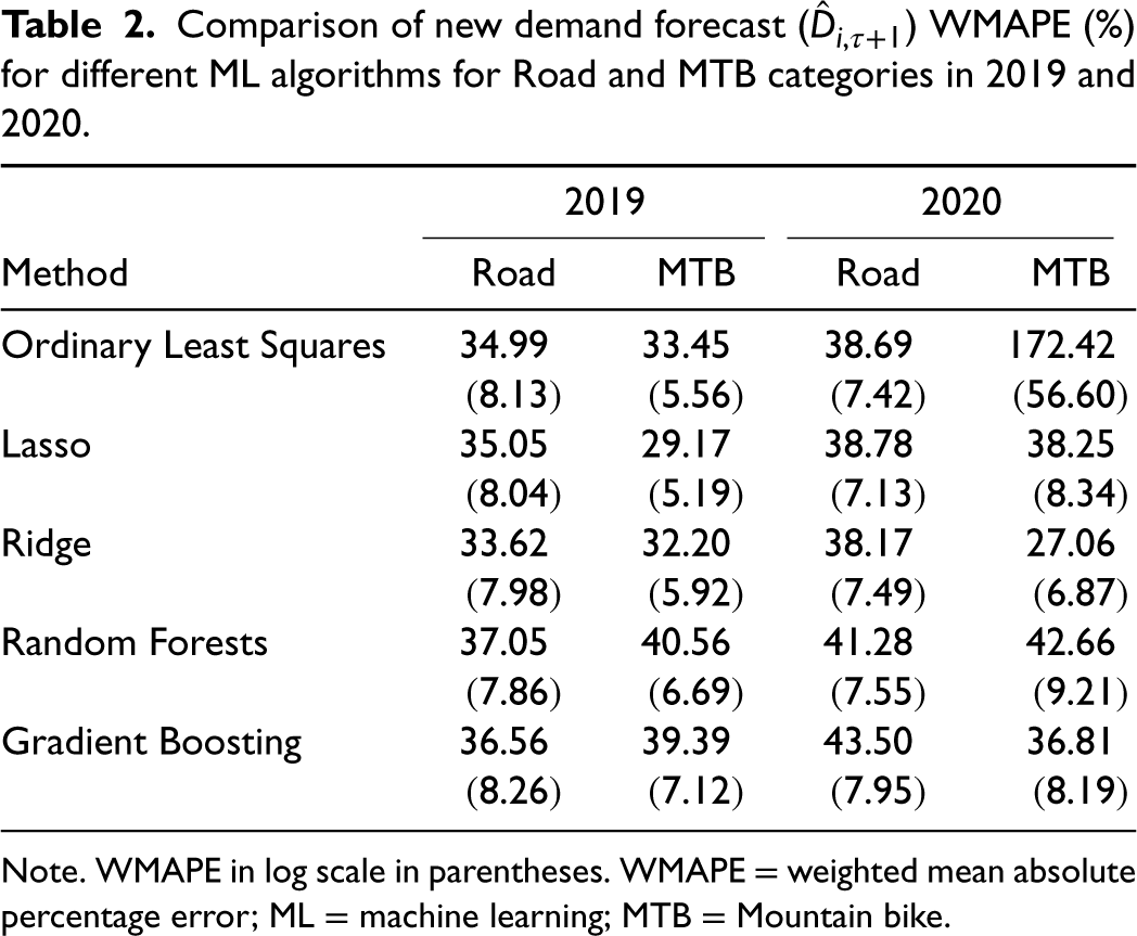
We validate the robustness of our integrated approach by forecasting the demand for Road and Mountain bike (MTB) categories for two consecutive seasons, 2019 and 2020, using the steps shown in the previous section. Table 2 compares the different ML models in terms of WMAPE.

Table 2.
Comparison of new demand forecast ( ${\hat{D}}_{i, τ + 1}$ ) WMAPE (%) for different ML algorithms for Road and MTB categories in 2019 and 2020.

2019 2020

Method Road MTB Road MTB

Ordinary Least Squares 34.99 33.45 38.69 172.42

(8.13) (5.56) (7.42) (56.60)

Lasso 35.05 29.17 38.78 38.25

(8.04) (5.19) (7.13) (8.34)

Ridge 33.62 32.20 38.17 27.06

(7.98) (5.92) (7.49) (6.87)

Random Forests 37.05 40.56 41.28 42.66

(7.86) (6.69) (7.55) (9.21)

Gradient Boosting 36.56 39.39 43.50 36.81

(8.26) (7.12) (7.95) (8.19)

	2019	2020
Ordinary Least Squares	34.99	33.45	38.69	172.42
	(8.13)	(5.56)	(7.42)	(56.60)
Lasso	35.05	29.17	38.78	38.25
	(8.04)	(5.19)	(7.13)	(8.34)
Ridge	33.62	32.20	38.17	27.06
	(7.98)	(5.92)	(7.49)	(6.87)
Random Forests	37.05	40.56	41.28	42.66
	(7.86)	(6.69)	(7.55)	(9.21)
Gradient Boosting	36.56	39.39	43.50	36.81
	(8.26)	(7.12)	(7.95)	(8.19)

Note. WMAPE in log scale in parentheses. WMAPE = weighted mean absolute percentage error; ML = machine learning; MTB = Mountain bike.

The Ridge regression model performs the best overall with a WMAPE of 7%, on average, on the log scale, which on re-transforming to the original scale of demand, gives us a WMAPE of 33% (WMAPE is 30% for products without stockouts and 34% for products with stockouts). The Ridge regression model is suitable in practical settings due to low computation effort and ease of interpretation. It also allows us to examine the relationship between demand and other variables from the model coefficients. The coefficients of the Ridge regression model are shrunk toward zero to achieve a lower variance at the cost of a slight increase in bias, thus ensuring the model generalizes well on new data. The final values of the tuning parameter $λ$ , obtained from cross-validation on the training data, that controls the shrinkage of the coefficients are reported in Table 3. More complex models, such as Random Forests or Gradient Boosting, do not lead to a further reduction in forecast errors.

Table 3.

Selected Ridge regression tuning parameter $λ$ with smallest cross-validation WMAPE for training data from 2018 to 2019.

	2018		2019
Tuning parameter	Road	MTB	Road	MTB
$λ$	0.148	0.215	0.260	0.285

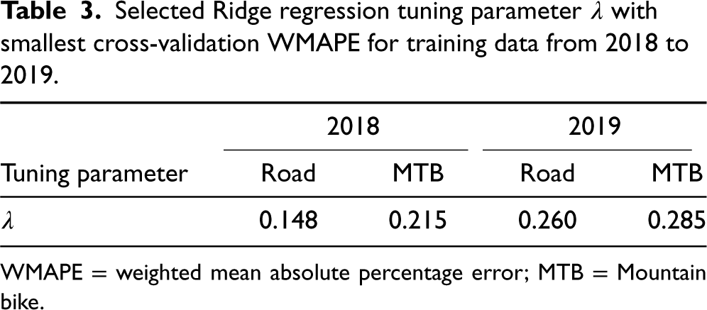
WMAPE = weighted mean absolute percentage error; MTB = Mountain bike.

We also calculate 95% prediction intervals to indicate confidence in the forecasts for the new season in order to enable inventory management decisions by the company. Assuming that the demand distribution is normal, a two-sided $100 (1 - α)$ prediction interval can be obtained as $F o r e c a s t \pm z_{α / 2} \times σ$ . In reality, the standard deviation $σ$ is typically unknown, and therefore RMSE values can be used instead (Ord et al., 2017). Figure 7 compares the mean demand forecasts and 95% prediction intervals with the true demand in 2019 and 2020. Additionally, in Table 4 we report the “coverage” resulting from the 95% interval on new data, i.e., the proportion of new observations that actually lie within the 95% interval. On average, we obtain 89% coverage across Road and MTB bikes in 2019 and 2020. We go a step further to analyze whether the coverage varies across quantiles of demand. We divide the demand forecast into four equal parts or quartiles and calculate the coverage for each quartile, as shown in Figure 8.

Figure 7.

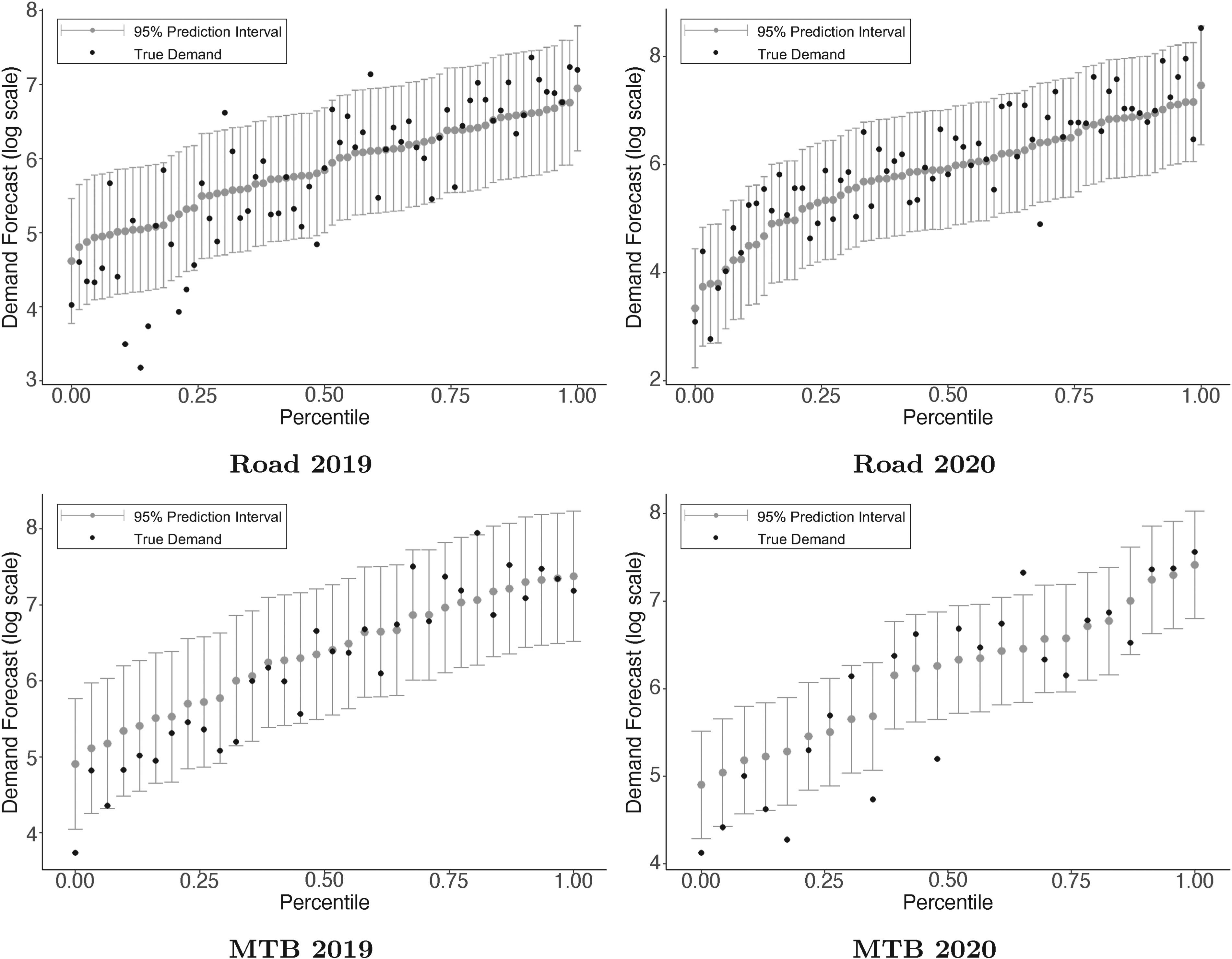
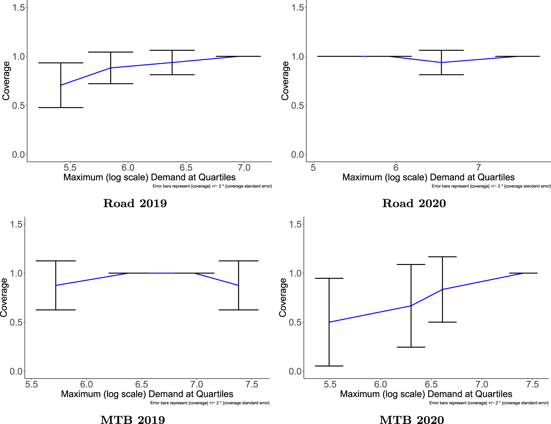
Prediction intervals for demand forecasts ${\hat{D}}_{i, τ + 1}$ and true demand $D_{i, τ + 1}$ for Road and Mountain bike (MTB) categories in 2019 and 2020.

Figure 8.

Coverage by quartiles for demand forecasts for Road and Mountain bike (MTB) categories in 2019 and 2020.

Table 4.

Demand coverage for Road and Mountain bike (MTB) categories in 2019 and 2020.

	2019		2020
Metric	Road	MTB	Road	MTB
Coverage (%)	88.06	93.75	98.51	75.00
$p$ -value for quantile differences	0.052	0.545	0.357	0.217

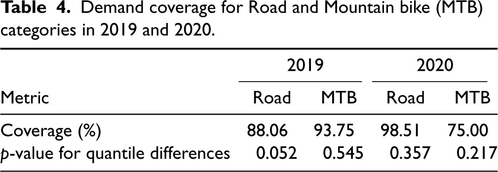
We can see that the coverage does not vary much by quantiles. For the Road category in 2020, the coverage is especially good across all quantiles. However, in 2019, the coverage is slightly lower for low-volume bikes, which is also observed in the case of the MTB category in 2020. A chi-squared test reveals whether the demand for the bike being covered by the prediction interval depends on which quantile it falls in. 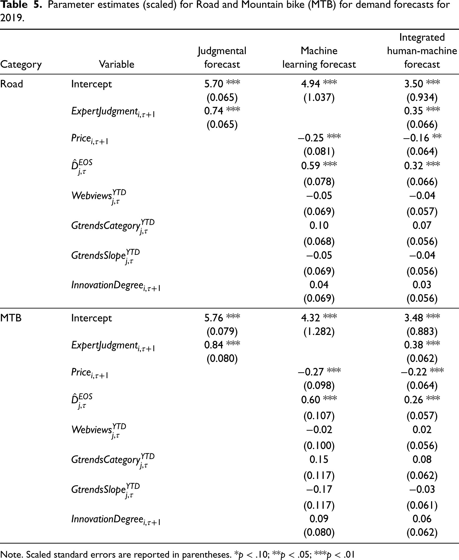The $p$ -values obtained from the test in Table 4 show that the coverage does not depend on the quantile.

6.1. The Value of Expert Judgment

Tables 5 - 6 summarize the scaled parameter estimates of (i) judgmental forecast, (ii) ML forecast, and (iii) integrated human-machine forecast, trained on data from 2018 (to forecast for 2019), and 2019 (to forecast for 2020). We can see that experts’ input is significant both in the single variable model and the integrated model. The coefficient estimates for the expert forecast lie between 0 and 1 in all cases, which indicates that the relation between the expert forecast and demand is not linear (due to the log-log formulation), but experts are more optimistic about high-volume bikes and tend to forecast higher than the actual demand for these bikes. For this reason, we also test the model performance after including the sales volume as a feature but do not see a significant improvement in forecast accuracy (refer to E-Companion section EC.4 for more details).

Table 5.
Parameter estimates (scaled) for Road and Mountain bike (MTB) for demand forecasts for 2019.

Category Variable Judgmental forecast Machine learning forecast Integrated human-machine forecast

Road Intercept 5.70 * 4.94 * 3.50 *

(0.065) (1.037) (0.934)

$E x p e r t J u d g m e n t_{i, τ + 1}$ 0.74 * 0.35 *

(0.065) (0.066)

$P r i c e_{i, τ + 1}$ $-$ 0.25 * $-$ 0.16

(0.081) (0.064)

${\hat{D}}_{j, τ}^{E O S}$ 0.59 * 0.32 *

(0.078) (0.066)

$W e b v i e w s_{j, τ}^{Y T D}$ $-$ 0.05 $-$ 0.04

(0.069) (0.057)

$G t r e n d s C a t e g o r y_{j, τ}^{Y T D}$ 0.10 0.07

(0.068) (0.056)

$G t r e n d s S l o p e_{j, τ}^{Y T D}$ $-$ 0.05 $-$ 0.04

(0.069) (0.056)

$I n n o v a t i o n D e g r e e_{i, τ + 1}$ 0.04 0.03

(0.069) (0.056)

MTB Intercept 5.76 * 4.32 * 3.48 *

(0.079) (1.282) (0.883)

$E x p e r t J u d g m e n t_{i, τ + 1}$ 0.84 * 0.38 *

(0.080) (0.062)

$P r i c e_{i, τ + 1}$ $-$ 0.27 * $-$ 0.22 *

(0.098) (0.064)

${\hat{D}}_{j, τ}^{E O S}$ 0.60 * 0.26 *

(0.107) (0.057)

$W e b v i e w s_{j, τ}^{Y T D}$ $-$ 0.02 0.02

(0.100) (0.056)

$G t r e n d s C a t e g o r y_{j, τ}^{Y T D}$ 0.15 0.08

(0.117) (0.062)

$G t r e n d s S l o p e_{j, τ}^{Y T D}$ $-$ 0.17 $-$ 0.03

(0.117) (0.061)

$I n n o v a t i o n D e g r e e_{i, τ + 1}$ 0.09 0.06

(0.080) (0.062)

Category	Variable	Judgmental forecast	Machine learning forecast	Integrated human-machine forecast
Road	Intercept	5.70 ***	4.94 ***	3.50 ***
		(0.065)	(1.037)	(0.934)
	$E x p e r t J u d g m e n t_{i, τ + 1}$	0.74 ***		0.35 ***
		(0.065)		(0.066)
	$P r i c e_{i, τ + 1}$		$-$ 0.25 ***	$-$ 0.16 **
			(0.081)	(0.064)
	${\hat{D}}_{j, τ}^{E O S}$		0.59 ***	0.32 ***
			(0.078)	(0.066)
	$W e b v i e w s_{j, τ}^{Y T D}$		$-$ 0.05	$-$ 0.04
			(0.069)	(0.057)
	$G t r e n d s C a t e g o r y_{j, τ}^{Y T D}$		0.10	0.07
			(0.068)	(0.056)
	$G t r e n d s S l o p e_{j, τ}^{Y T D}$		$-$ 0.05	$-$ 0.04
			(0.069)	(0.056)
	$I n n o v a t i o n D e g r e e_{i, τ + 1}$		0.04	0.03
			(0.069)	(0.056)
MTB	Intercept	5.76 ***	4.32 ***	3.48 ***
		(0.079)	(1.282)	(0.883)
	$E x p e r t J u d g m e n t_{i, τ + 1}$	0.84 ***		0.38 ***
		(0.080)		(0.062)
	$P r i c e_{i, τ + 1}$		$-$ 0.27 ***	$-$ 0.22 ***
			(0.098)	(0.064)
	${\hat{D}}_{j, τ}^{E O S}$		0.60 ***	0.26 ***
			(0.107)	(0.057)
	$W e b v i e w s_{j, τ}^{Y T D}$		$-$ 0.02	0.02
			(0.100)	(0.056)
	$G t r e n d s C a t e g o r y_{j, τ}^{Y T D}$		0.15	0.08
			(0.117)	(0.062)
	$G t r e n d s S l o p e_{j, τ}^{Y T D}$		$-$ 0.17	$-$ 0.03
			(0.117)	(0.061)
	$I n n o v a t i o n D e g r e e_{i, τ + 1}$		0.09	0.06
			(0.080)	(0.062)

Note. Scaled standard errors are reported in parentheses. * $p < .10$ ; ** $p < .05$ ; *** $p < .01$

Table 6.

Parameter estimates (scaled) for Road and Mountain bike (MTB) category for demand forecasts for 2020.

Category	Variable	Judgmental forecast	Machine learning forecast	Integrated human-machine forecast
Road	Intercept	5.71 ***	1.69 *	1.21
		(0.078)	(0.929)	(0.906)
	$E x p e r t J u d g m e n t_{i, τ + 1}$	0.82 ***		0.26 ***
		(0.079)		(0.060)
	$P r i c e_{i, τ + 1}$		$-$ 0.18 **	$-$ 0.12 **
			(0.068)	(0.061)
	${\hat{D}}_{j, τ}^{E O S}$		0.39 ***	0.27 ***
			(0.072)	(0.062)
	$W e b v i e w s_{j, τ}^{Y T D}$		0.38 ***	0.27 ***
			(0.069)	(0.061)
	$G t r e n d s C a t e g o r y_{j, τ}^{Y T D}$		0.01	$-$ 0.01
			(0.065)	(0.059)
	$G t r e n d s S l o p e_{j, τ}^{Y T D}$		0.07	0.04
			(0.066)	(0.059)
	$I n n o v a t i o n D e g r e e_{i, τ + 1}$		0.04	0.03
			(0.064)	(0.058)
MTB	Intercept	5.93 ***	2.58 ***	2.02 **
		(0.076)	(0.892)	(0.844)
	$E x p e r t J u d g m e n t_{i, τ + 1}$	0.95 ***		0.33 ***
		(0.078)		(0.046)
	$P r i c e_{i, τ + 1}$		$-$ 0.21 ***	$-$ 0.16 **
			(0.065)	(0.058)
	${\hat{D}}_{j, τ}^{E O S}$		0.36 ***	0.26 ***
			(0.066)	(0.061)
	$W e b v i e w s_{j, τ}^{Y T D}$		0.33 ***	0.20 ***
			(0.066)	(0.056)
	$G t r e n d s C a t e g o r y_{j, τ}^{Y T D}$		$-$ 0.21 ***	$-$ 0.17 ***
			(0.055)	(0.049)
	$G t r e n d s S l o p e_{j, τ}^{Y T D}$		$-$ 0.12 **	$-$ 0.06
			(0.042)	(0.038)
	$I n n o v a t i o n D e g r e e_{i, τ + 1}$		0.04	0.02
			(0.051)	(0.047)

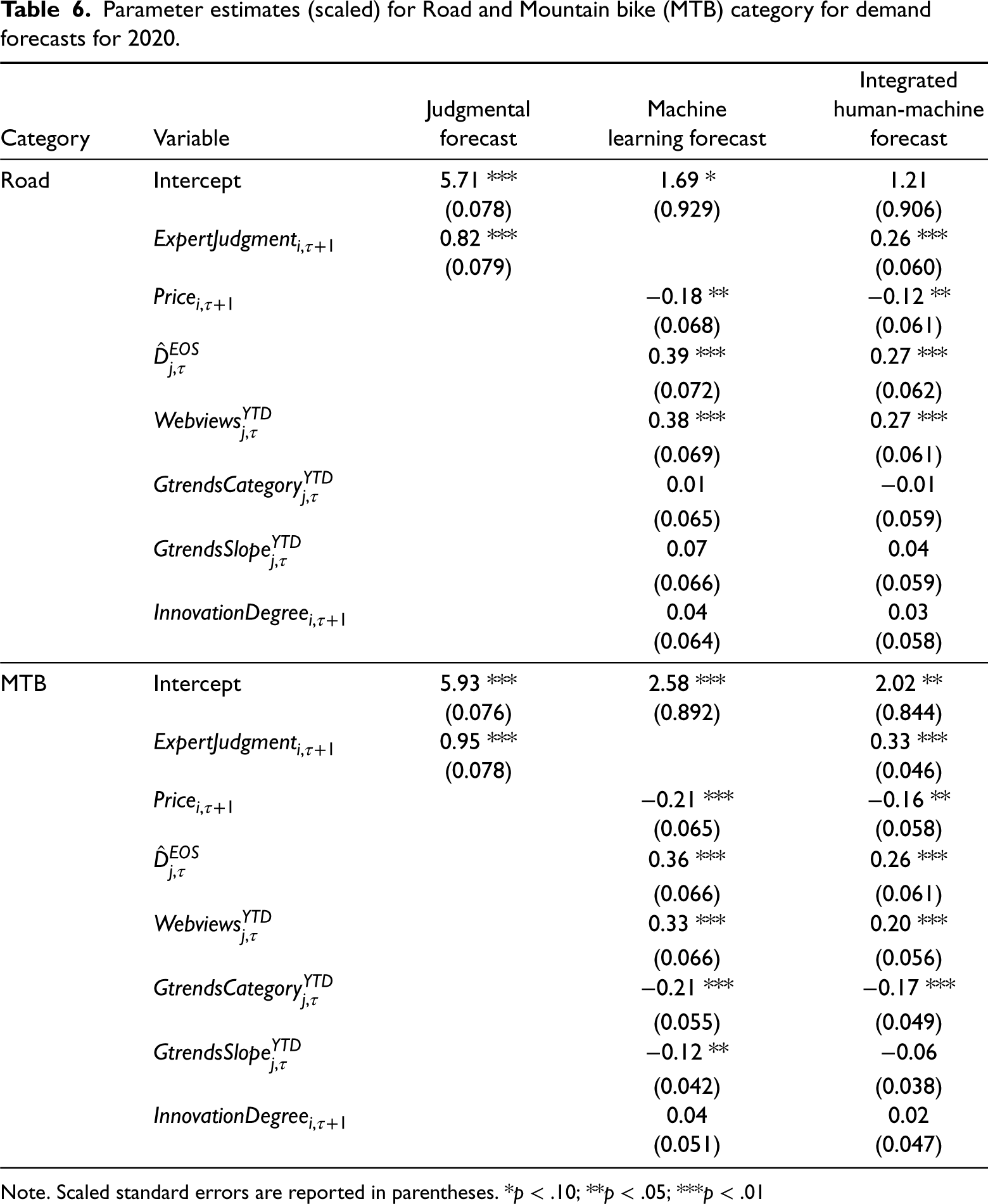
Note. Scaled standard errors are reported in parentheses. * $p < .10$ ; ** $p < .05$ ; *** $p < .01$

The price and end-of-season true demand estimate are significant variables across all datasets. The price of the bike in the new season is an important feature as price fluctuations are common for innovative products and even in cases where the products are not completely new, any change in the price of the product has a big impact on the demand. Additionally, our study shows that leveraging the most recent information available in terms of the end-of-the-current season demand forecast is advantageous. We find that using this estimate as a feature in our model results in a 5% improvement in WMAPE as compared to including only the sales of the bikes until the point of forecasting. We also note that web traffic data is significant in the case of models trained on 2019 data but not on 2018 data.

In addition to the coefficients, we calculate the permutation feature importance for the integrated human-machine forecast and the ML forecast in Figure 9. Permutation feature importance is model-agnostic and an intuitive way to identify which features are most important in the model. They are obtained by shuffling the column containing the particular feature and making predictions using the model on the shuffled data. A higher value of feature importance indicates that the feature is very important for the model to make predictions and to generalize to unseen data. From Figure 9, we observe that expert judgment and the total end-of-season demand are the two most important features for all categories and the expert judgment is the most valuable in the integrated human-machine forecast model for all cases except one. We also calculate feature importance based on SHAP values which is shown to be more robust in the presence of correlated features. We obtain the same results using this approach as well (E-Companion section EC.5 illustrates the SHAP values for features from the different forecasting methods.)

Figure 9.

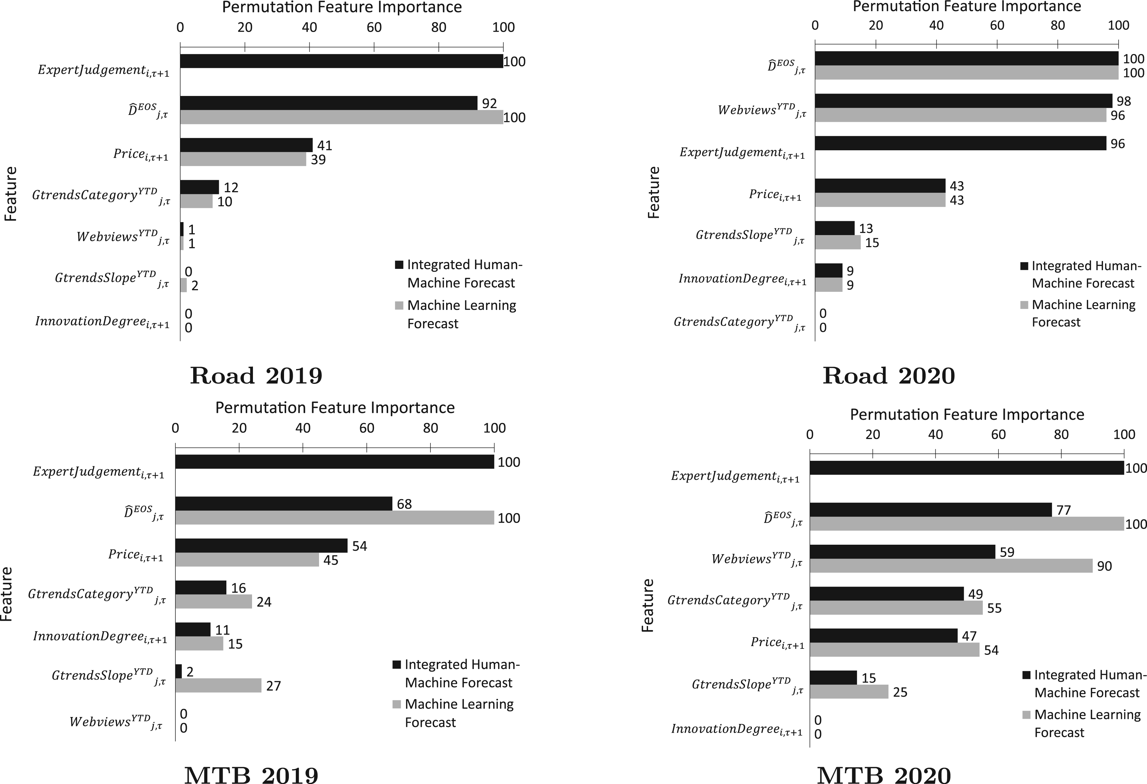
Comparison of permutation feature importance for integrated human-machine demand forecasts vs. ML forecasts for 2019 and 2020.

We also analyze how the permutation feature importance changes based on the product characteristics measured by the innovation degree variable, which represents how different the new product is in terms of its components as compared to an older version. From Figure 10, we find that the importance of expert judgment increases for newer products (i.e., as the innovation degree increases). In contrast, the importance of historical demand depicted by the total end-of-season true demand decreases for newer products. This is also true for other statistical features apart from certain Google Trends features which increase as the degree of innovation increases. Although only limited data was available for this analysis⁴, we can remark that the expert judgment proves valuable for more innovative products. Meanwhile, historical data has more importance for products that get carried over to the next season with little changes.

Figure 10.

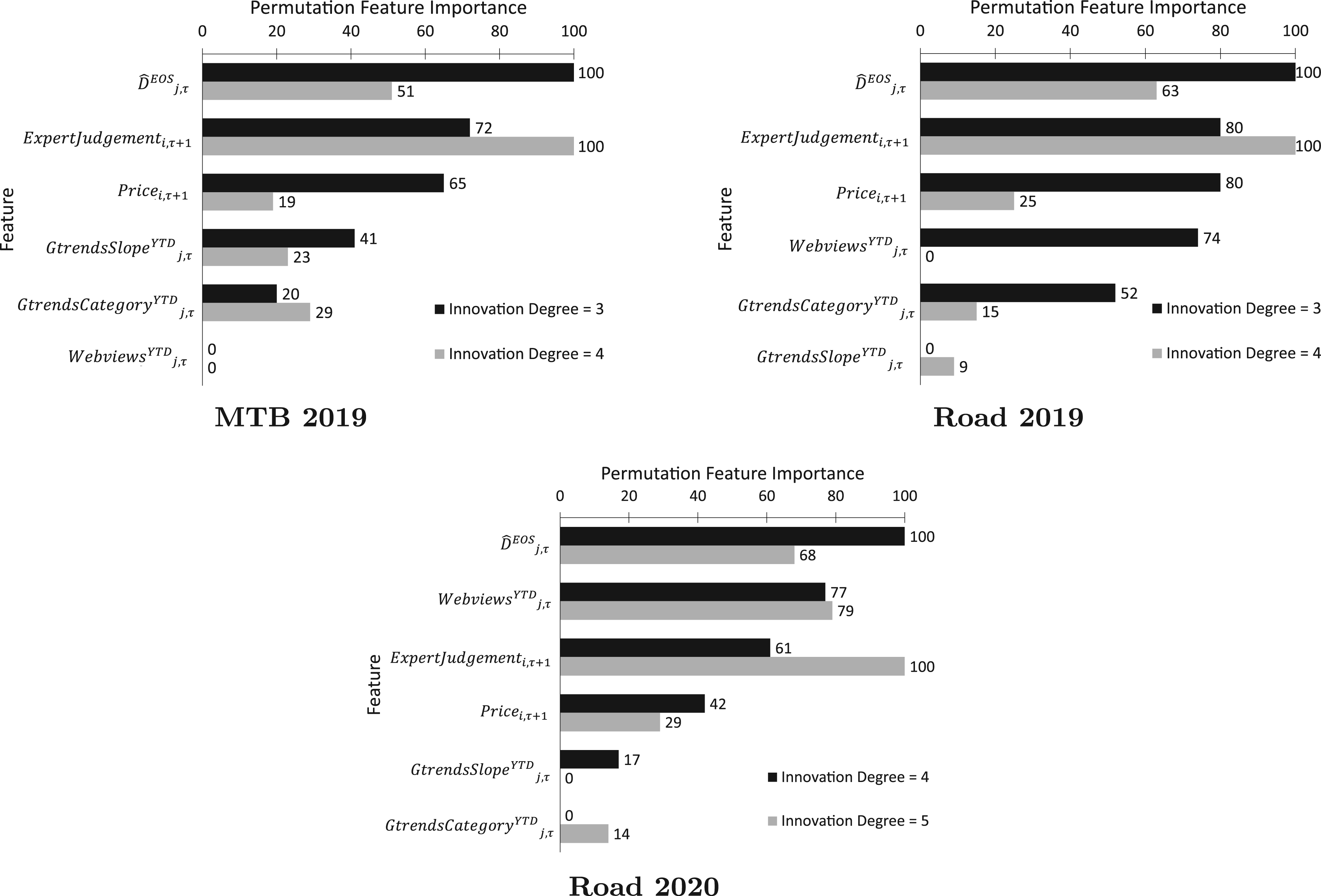
Comparison of permutation feature importance for expert judgment and statistical features based on varying innovation degrees.

The forecast accuracies in terms of WMAPE for all the methods are reported in Table 7. The relative improvement in forecasting accuracy averaged over all test cases, is calculated using Equation 10. The bias-corrected judgmental forecast using the log-log model with only the expert input has a 20% lower WMAPE as compared to a pure judgmental forecast. The ML prediction has a 24% lower WMAPE than the pure judgmental forecast and the integrated human-machine forecast results in a further 14% reduction in WMAPE. The log scale integrated model and pure judgmental forecasts for 2019 and 2020 are presented in Figure 11.

\begin{aligned} RelativeImprovement = \frac{{WMAPE}_{M e t h o d 1} - {WMAPE}_{M e t h o d 2}}{{WMAPE}_{M e t h o d 1}} \end{aligned}

(10)

Figure 11.

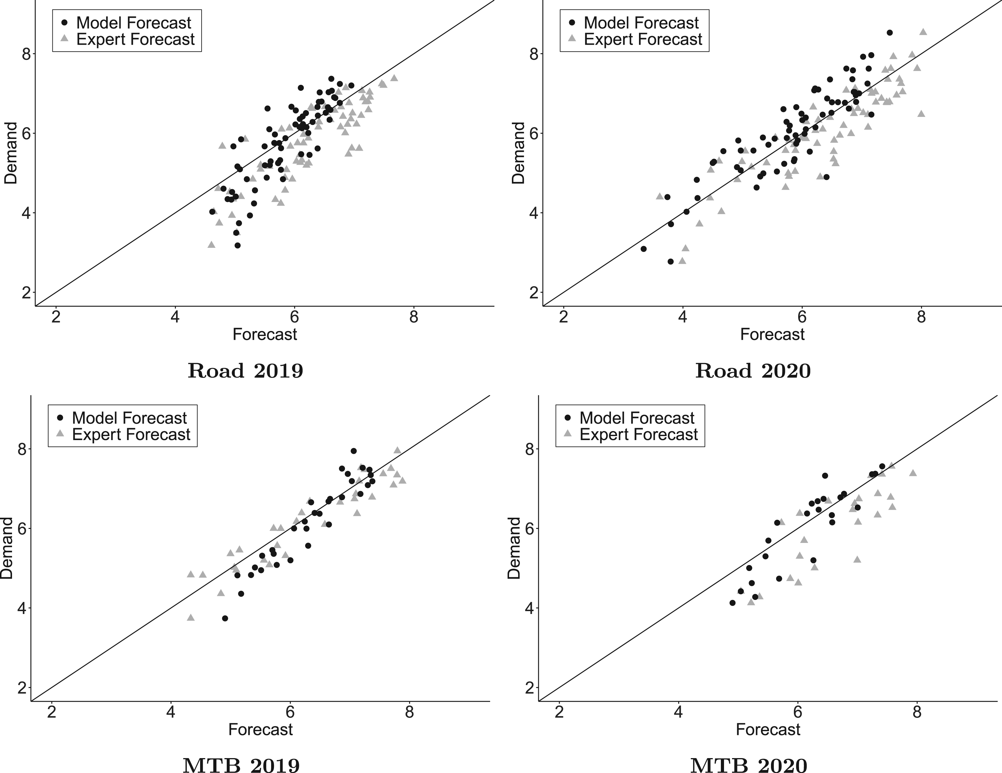
Comparison of model and expert forecasts in log scale for 2019 and 2020.

Table 7.

Average relative improvement in forecast accuracy on predictions for 2019 and 2020.

Forecasting method	Weighted mean absolute percentage error (WMAPE) (%)	Relative improvement over judgmental forecast (%)	Relative improvement over machine learning forecast (%)
Pure judgmental forecast	50	-	-
Bias-corrected judgmental forecast	40	20**	-
Machine learning forecast	38	24***	-
Integrated human-machine forecast	33	35***	14

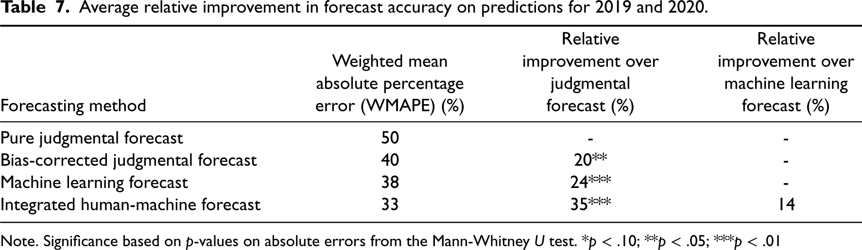
Note. Significance based on $p$ -values on absolute errors from the Mann-Whitney $U$ test. * $p < .10$ ; ** $p < .05$ ; *** $p < .01$

These findings prove that judgmental forecast continues to play a critical role even in the presence of advanced statistical tools and increasing data availability. This can be explained by the fact that experts have access to timely contextual information, which is particularly important for rapid innovations, where new attributes are continuously added through the latest technology or advanced raw materials. This type of information is often kept in secrecy before the launch of the new season and determines the company’s competitive edge. At Canyon Bicycles, the innovations are only revealed to internal and external stakeholders in the first week of the season. Besides new technology in the market, experts also have knowledge of special events (e.g., sporting events⁵ ), changes in regulations, and sudden shifts in consumer preference. This type of information is difficult for any ML algorithm to capture as these models can only predict based on what has happened in the past. In addition, experts possess the ability to alter their judgment in response to disruptions quickly. During the COVID-19 pandemic, judgmental forecasts inevitably replaced statistical models that could not cope with the unforeseen crisis. However, judgmental forecasts alone do not result in accurate forecasts, and we need ML models that can leverage historical data and provide predictions that overcome the biases in expert forecasts. Therefore, ML methods act as drivers for developing accurate forecasts, and a combination of the two methods is recommended to forecast the demand for innovative products.

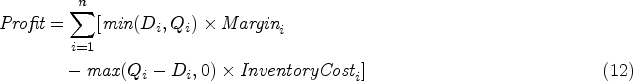
6.2. Service Level and Optimal Order Quantity

For a company operating in a fiercely competitive market such as Canyon Bicycles, any improvement in forecasting accuracy has a direct impact on the business. Many of its competitors have gone bankrupt in the past as they could not keep up with the exploding growth of the bicycle industry. At the same time, excess inventory needs to be cleared off before the new season’s stock comes in. Moreover, the bicycle industry is currently facing an excess inventory problem as a consequence of building up inventory during the supply disruptions caused by the pandemic recently (for example, Giant⁶ and Rose Bikes⁷). Therefore, while making ordering decisions for the new season, a trade-off between overage and underage costs needs to be made. This is typically done using the Newsvendor model, which equates expected gain to expected loss on a product to obtain the profit-maximizing order quantity.

At Canyon Bicycles, the underage costs given by the profit margin are 41% for MTB bikes and 38% for Road bikes. The overage costs are roughly 50% of the manufacturing costs (see Diermann and Huchzermeier, 2017). The service level for Road bikes is then calculated as 55% and for MTB bikes as 58%. Therefore, we can compute the optimal order quantity $Q_{i, τ + 1}$ for product $i$ in season $τ + 1$ as:

Q_{i, τ + 1} = e x p ({\hat{D}}_{i, τ + 1}^{l o g} + z \times σ_{i, τ + 1})

(11)

where

{\hat{D}}_{i, τ + 1}^{l o g}

is the mean demand forecast for product

i

in the new season

τ + 1

in log-scale, and

σ_{i, τ + 1}

represents the standard deviation of the log demand distribution, as calculated in Section 6.

z

can be estimated from the service level or the critical ratio

(c_{u} / c_{o} + c_{u})

using the Standard Normal Distribution Table (since the demand distribution is normal in the logarithmic scale).

On comparing the order quantities calculated from the integrated human-machine forecast to the ones calculated from purely judgmental forecasts, we observe that the experts overestimate the demand in the new season, which, on the one hand, reduces lost sales, but, on the other hand, increases leftover inventory. The human-machine forecasts, in contrast, lead to less leftover inventory. Overall, based on the calculation of gross profits for seasons 2019 and 2020 using Equation 12, which takes into account both lost profits and the cost of excess inventory, we find that the integrated human-machine forecast results in a 28% higher profit as compared to the pure judgmental forecast and a 5% higher profit as compared to the bias-corrected judgmental forecast.

\begin{aligned} Profit & = \sum_{i = 1}^{n} [min (D_{i}, Q_{i}) \times {Margin}_{i} \\ - max (Q_{i} - D_{i}, 0) \times {InventoryCost}_{i}] \end{aligned}

(12)

7. Conclusion

Demand forecasting for new products is a challenge faced by many companies. Moreover, forecast accuracy tends to be relatively lower for fast innovations compared to less innovative products with long life cycles. This issue is encountered by many companies, particularly within the fashion and high-tech industry where products have short selling seasons and unpredictable demand. Prediction accuracy becomes even more critical when forecasts need to be finalized several months before the start of the season. Through an empirical analysis, we highlight these challenges unique to innovation-driven companies. In our paper, we show the value of combining ML models with the experts’ knowledge of the market. We find that the integrated human-machine forecast estimated using a Ridge regression reduces the forecast error, given by WMAPE, by 35% compared to a pure judgmental forecast in our dataset. Our study emphasizes the importance of expert judgment in forecasting. Experts are exposed to an infinite number of cues and have access to timely information, which is difficult to capture by statistical models. Furthermore, Goodwin (2002) notes that managers who are knowledgeable about their products are more likely to accept forecasts when they have participated in the process of deriving them. Our findings also show that experts’ input carries more weight than historical data for newer products. Therefore, we recommend that innovation-driven companies use advanced statistical learning models to support and evaluate expert judgments, not replace them.

Several other important insights emerge from our study. First, stockouts in the past should not be ignored as they bias sales and provide an unreliable anchor for forecasting demand in the future. Moreover, we found that customers may delay their purchase in the event of a stockout, making it extremely difficult to keep track of when substitution takes place. Additionally, while substitution happens, certain sizes (or SKUs) of substitute products also stock out, making the problem of tracking substitution even more complicated (refer to the E-Companion section EC1.1). Therefore, instead of calculating the substitute demand and lost sales separately, we directly calculate the true demand using ML. Any price reductions offered in the past should also be suitably handled if a company is only interested in predicting and ordering the base demand (refer to the E-Companion section EC.1.3). In contrast, the price of the product can be used as an additional variable in the true demand prediction model if sales uplift due to discounts is required. We also note that price is a significant feature in our model. Innovative products typically operate with high margins and prices change every season. Therefore, even for products that don’t change from one season to another, price changes have a significant impact on the demand. Additionally, our analysis shows that the end-of-season true demand estimate for a bike in the current season is a good indicator of demand for the upgraded model in the next season. Thus, leveraging past information on comparable bikes is indeed beneficial. Furthermore, a higher degree of innovation (i.e., the newer the product is) leads to higher demand. We also analyze the relationship between innovation degree and the importance given to the experts’ forecast. Our findings show that experts’ input is more valuable than historical data for newer products. Due to limited data available, we do not dive deeper into analyzing for which type of products expert judgment may even be worse and would be an interesting direction for future studies. We also report a 28% increase in profits on using our integrated approach. Therefore, for a company operating in an environment of high demand uncertainty and fierce competition, an improvement in forecasting accuracy translates to higher profits.

The models developed in this paper can be applied in any e-commerce firm as they are not computationally time-consuming and are easily interpretable in a business setting because of the regression formulation. Our study can be further generalized to different levels of product hierarchy depending on the company’s requirements and data availability. Here, we present our analysis at the product level, as in the case of Canyon Bicycles. The forecasts are derived at the bike model level and then further disaggregated to the SKU level. One of the challenges for companies to implement the models discussed in this paper is the maintenance of data. Since different functions within the organization generate different types of data – operational, online, market, and other data, a “data center” will make it easier to access all available data for a particular product in one click. This was implemented at Canyon Bicycles during the study. We also collected social media data from Instagram but did not include it in our model due to the sparseness of the data, with some bike families having no posts during the entire season. This forms a potential area for future research. Additional features can easily be incorporated into the model, leaving it to the ML algorithm to identify the most important features.

As our period of analysis extends into 2020, we need to mention the impact of the COVID-19 pandemic. The pandemic is known to have had a big impact on bike sales⁸. At the time of forecasting for 2020, we could not anticipate such a catastrophe to take place. Therefore, we denote it as a black swan event. To forecast demand for the future seasons, i.e., in the “new normal,” the pandemic impact since 2020 should be taken into account in the ML algorithms.

We do not consider the excess sales during the pandemic for testing our forecasting model for 2020. As it is not possible to isolate the impact of this event on the sales data, we apply the end-of-season true demand estimation model from Equation 5 on the initial sales data until March 2020, before the pandemic situation intensified to calculate the demand in a non-pandemic scenario. This is based on the assumption that, in the absence of the pandemic, the shape of the demand curve would fall into one of the bike clusters from the previous seasons (see Figure 6). This demand curve is illustrated in Figure 12. In addition, the figure also shows that we can calculate the true demand when a bike stocks out during the pandemic using the prediction model from Equation 2.

Figure 12.

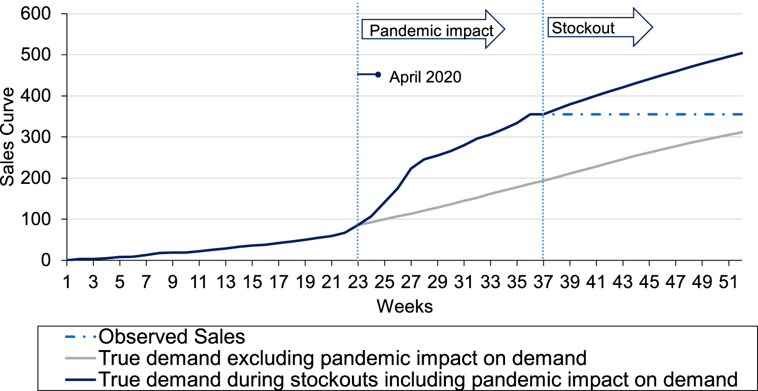
An example of different demand curves during the pandemic.

We do not know how the pandemic will affect sales in the future and therefore need to monitor it continuously. Companies around the world have experienced a continuum of crises for a very long time. The only way forward for companies is to learn from these events and improve their resilience strategy (Cohen et al., 2022). In order to forecast demand in such a setting, all previous decisions become part of the expert’s information set, which they can rely on to improve their forecasts for the new seasons. Thus, the involvement of expert judgment becomes even more crucial during these circumstances.

Supplemental Material

sj-pdf-1-pao-10.1177_10591478241245138 - Supplemental material for Predictably Unpredictable? How Judgmental and Machine Learning Forecasts Complement Each Other

Supplemental material, sj-pdf-1-pao-10.1177_10591478241245138 for Predictably Unpredictable? How Judgmental and Machine Learning Forecasts Complement Each Other by Devadrita Nair and Arnd Huchzermeier in Production and Operations Management

Footnotes

Appendix

Acknowledgments

The authors thank Daniela Laprell, Daniela Hofmann and André Janisch from the Business Intelligence Team at Canyon Bicycles for sharing the data for this study and for the valuable discussions. We also thank the reviewers and the senior and department editors for their recommendations that significantly enhanced the analysis and presentation of the paper.

Declaration of Conflicting Interests

The authors declared no potential conflicts of interest with respect to the research, authorship, and/or publication of this article.

Funding

The authors received no financial support for the research, authorship and/or publication of this article.

ORCID iDs

Devadrita Nair

Arnd Huchzermeier

Supplemental Material

Supplemental material for this article is available online (doi: ).

Notes

How to cite this article

Nair D, Huchzermeier A (2024) Predictably Unpredictable? How Judgmental and Machine Learning Forecasts Complement Each Other. Production and Operations Management 33(5): 1214–1234.

References

Abdallah

Vulcano

(2021) Demand estimation under the multinomial logit model from sales transaction data. Manufacturing & Service Operations Management 23(5): 1196–1216.

Aouad

Feldman

Segev

, et al. (2019) Click-Based MNL: Algorithmic Frameworks for Modeling Click Data in Assortment Optimization, Available at SSRN: https://ssrn.com/abstract=3340620.

Arvan

Fahimnia

Reisi

, et al. (2019) Integrating human judgement into quantitative forecasting methods: A review. Omega 86: 237–252.

Baardman

Levin

Perakis

, et al. (2018) Leveraging comparables for new product sales forecasting. Production and Operations Management 27(12): 2340–2343.

Bansal

Gutierrez

(2020) Estimating uncertainties using judgmental forecasts with expert heterogeneity. Operations Research 68(2): 363–380.

Blattberg

Hoch

(1990) Database models and managerial intuition: 50% model + 50% manager. Management Science 36(8): 887–899.

Cachon

Terwiesch

(2013) Matching Supply with Demand : An Introduction to Operations Management. 3rd ed. New York, NY: McGraw-Hill.

Cohen

Cui

Doetsch

, et al. (2022) Bespoke supply-chain resilience: The gap between theory and practice. Journal of Operations Management 68(5): 515–531.

Cohen

Leung

N-HZ

Panchamgam

, et al. (2017) The impact of linear optimization on promotion planning. Operations Research 65(2): 446–468.

10.

Conlon

Mortimer

(2013) Demand estimation under incomplete product availability. American Economic Journal: Microeconomics 5(4): 1–30.

11.

Cowgill

Zitzewitz

(2015) Corporate prediction markets: Evidence from google, ford, and firm X. The Review of Economic Studies 82(4): 1309–1341.

12.

Diermann

Huchzermeier

(2016a) Estimating Demand Uncertainty Using Dispersion of Team Forecasts or Distributions of Forecast Errors, Available at SSRN: https://ssrn.com/abstract=2782402.

13.

Diermann

Huchzermeier

(2016b) Judgmental Demand Forecasting for Online Sales of Product Collections: Segmentation by Type or Age?, Available at SSRN: https://ssrn.com/abstract=2782002.

14.

Diermann

Huchzermeier

(2017) Case—Canyon bicycles: Judgmental demand forecasting in direct sales. INFORMS Transactions on Education 17(2): 63–74.

15.

Duan

(1983) Smearing estimate: A nonparametric retransformation method. Journal of the American Statistical Association 78(383): 605–610.

16.

ECR Australia (2010) Winning with promotions industry report.

17.

Ferreira

Lee

BHA

Simchi-Levi

(2016) Analytics for an online retailer: Demand forecasting and price optimization. Manufacturing & Service Operations Management 18(1): 69–88.

18.

Fildes

Goodwin

(2007) Against your better judgment? how organizations can improve their use of management judgment in forecasting. INFORMS Journal on Applied Analytics 37(6): 570–576.

19.

Fildes

Goodwin

Lawrence

, et al. (2009) Effective forecasting and judgmental adjustments: An empirical evaluation and strategies for improvement in supply-chain planning. International Journal of Forecasting 25(1): 3–23.

20.

Fisher

Hammond

Obermeyer

, et al. (1994) Making supply meet demand in an uncertain world. Harvard Business Review 72: 83–83.

21.

Fisher

Raman

(1996) Reducing the cost of demand uncertainty through accurate response to early sales. Operations Research 44(1): 87–99.

22.

Fisher

Raman

(2018) Using data and big data in retailing. Production and Operations Management 27(9): 1665–1669.

23.

Gaur

Kesavan

Raman

, et al. (2007) Estimating demand uncertainty using judgmental forecasts. Manufacturing & Service Operations Management 9(4): 480–491.

24.

Goodwin

(1997) Adjusting judgemental extrapolations using theil’s method and discounted weighted regression. Journal of Forecasting 16(1): 37–46.

25.

Goodwin

(2002) Integrating management judgment and statistical methods to improve short-term forecasts. Omega 30(2): 127–135.

26.

Griffin

Brenner

(2004) Perspectives on Probability Judgment Calibration. Blackwell Handbook of Judgment and Decision Making, chap. 9. John Wiley & Sons, Ltd, 177–199.

27.

Hastie

Tibshirani

Friedman

(2009) Model Assessment and Selection. The Elements of Statistical Learning: Data Mining, Inference, and Prediction. Springer Series in Statistics, Springer, New York, 219–259.

28.

T-H

Chen

K-Y

(2007) New product blockbusters: The magic and science of prediction markets. California Management Review 50(1): 144–158.

29.

Acimovic

Erize

, et al. (2019) Forecasting new product life cycle curves. Manufacturing & Service Operations Management 21(1): 66–85.

30.

Hyndman

Athanasopoulos

(2018) Forecasting: Principles and Practice. OTexts: Melbourne, Australia. https://otexts.com/fpp2/. Accessed on 15 November 2021.

31.

Jain

Rudi

Wang

(2015) Demand estimation and ordering under censoring: Stock-out timing is (almost) all you need. Operations Research 63(1): 134–150.

32.

Kahn

(2002) An exploratory investigation of new product forecasting practices. Journal of Product Innovation Management 19(2): 133–143.

33.

Kahn

Charles

W Chase

(2018) The state of new-product forecasting. Foresight: The International Journal of Applied Forecasting, International Institute of Forecasters (51): 24–31. https://ideas.repec.org/a/for/ijafaa/y2018i51p24-31.html

34.

Kök

Fisher

(2007) Demand estimation and assortment optimization under substitution: Methodology and application. Operations Research 55(6): 1001–1021.

35.

Lawrence

Goodwin

O’Connor

(2006) Judgmental forecasting: A review of progress over the last 25 years. International Journal of Forecasting 22(3): 493–518.

36.

Lee

(2002) Aligning supply chain strategies with product uncertainties. California Management Review 44(3): 105–119.

37.

Matthias

Seifert

Siemsen

Enno

Hadida

Allègre L

, et al. (2015) Effective judgmental forecasting in the context of fashion products. Journal of Operations Management 36(1): 33–45.

38.

Ord

Fildes

Kourentzes

(2017) Principles of business forecasting.

39.

Ratliff

Venkateshwara Rao

Narayan

, et al. (2008) A multi-flight recapture heuristic for estimating unconstrained demand from airline bookings. Journal of Revenue and Pricing Management 7(2): 153–171.

40.

Ritchie

Mathieu

Rodés-Guirao

, et al. (2020) Coronavirus pandemic (COVID-19). http://ourworldindata.org/coronavirus. Last accessed 21 November 2021.

41.

Sanders

Ritzman

(2004) Integrating judgmental and quantitative forecasts: Methodologies for pooling marketing and operations information. International Journal of Operations & Production Management 24(5): 514–529.

42.

Simchi-Levi

Timmermans

(2021) A simpler way to modernize your supply chain. Harvard Business Review. https://hbr.org/2021/09/a-simpler-way-to-modernize-your-supply-chain

43.

Soule

Grushka-Cockayne

Merrick

(2023) A heuristic for combining correlated experts when there are few data. Management Science. https://pubsonline.informs.org/doi/full/10.1287/mnsc.2021.02009?casa_token=Zd6wf2ote1oAAAAA%3A4BpQXKBviyLFWCd3ENWCfEUFL3p0fSO3rR3-ggolRq0CcSMKP_ufKwkcMwOK2e3uonV7GDzL

44.

Trapero

Pedregal

Fildes

, et al. (2013) Analysis of judgmental adjustments in the presence of promotions. International Journal of Forecasting 29(2): 234–243.

45.

Vulcano

van Ryzin

Ratliff

(2012) Estimating primary demand for substitutable products from sales transaction data. Operations Research 60(2): 313–334.

46.

Wolters

Huchzermeier

(2021) Joint in-season and out-of-season promotion demand forecasting in a retail environment. Journal of Retailing 97(4): 726–745.

Supplementary Material

Please find the following supplemental material available below.

For Open Access articles published under a Creative Commons License, all supplemental material carries the same license as the article it is associated with.

For non-Open Access articles published, all supplemental material carries a non-exclusive license, and permission requests for re-use of supplemental material or any part of supplemental material shall be sent directly to the copyright owner as specified in the copyright notice associated with the article.

0.00 MB

1.06 MB

	2019		2020
Method	Road	MTB	Road	MTB
Ordinary Least Squares	34.99	33.45	38.69	172.42
	(8.13)	(5.56)	(7.42)	(56.60)
Lasso	35.05	29.17	38.78	38.25
	(8.04)	(5.19)	(7.13)	(8.34)
Ridge	33.62	32.20	38.17	27.06
	(7.98)	(5.92)	(7.49)	(6.87)
Random Forests	37.05	40.56	41.28	42.66
	(7.86)	(6.69)	(7.55)	(9.21)
Gradient Boosting	36.56	39.39	43.50	36.81
	(8.26)	(7.12)	(7.95)	(8.19)

Predictably Unpredictable? How Judgmental and Machine Learning Forecasts Complement Each Other

Abstract

Keywords

1. Introduction

2. Literature Review

3. The Integrated Demand Forecast for the New Season τ + 1

4.1. Estimation of True Demand during Stockouts (previous season τ − 1 )

Supplemental Material

sj-pdf-1-pao-10.1177_10591478241245138 - Supplemental material for Predictably Unpredictable? How Judgmental and Machine Learning Forecasts Complement Each Other

Footnotes

Appendix

Acknowledgments

Declaration of Conflicting Interests

Funding

ORCID iDs

Supplemental Material

Notes

How to cite this article

References

Supplementary Material

3. The Integrated Demand Forecast for the New Season $τ + 1$

4.1. Estimation of True Demand during Stockouts (previous season $τ - 1$ )