
Abstract
The bullwhip effect (BWE) is an important phenomenon in the operations and supply chain management field. Although it is commonly accepted that the BWE is widespread and can have a significant adverse impact on financial performance, there is surprisingly limited objective evidence on the financial consequences of the BWE. This paper examines the impact of the BWE on financial performance by examining the relationship between the BWE and stock price performance. The empirical analysis is based on data from 1985 to 2018 from about 7200 publicly traded firms and about 64,000 firm-years. We find that most results on the impact of the BWE on stock returns are statistically indistinguishable from zero. The few marginally significant results that we find suggest a positive relationship between the BWE and stock returns rather than the expected negative relationship. However, these marginally significant results do not hold when alternate methods are used to test the relationships. These conclusions are robust when we segment the sample by size, industry, and time periods. We also do not find a significant relationship between the BWE and stock returns for samples based on the propagation of the BWE from customers to suppliers. We do find some evidence to suggest that the BWE has a negative impact on inventory turnover. However, we do not find similar evidence for capacity utilization. The relationships between the BWE and return on assets measures are statistically insignificant. For margin measures, the relationships are positive and statistically significant but not economically significant.
Introduction
The bullwhip effect (BWE) is an important phenomenon in the operations and supply chain management field. The seminal paper of Lee et al. (1997a: 546) defined the BWE as “the phenomenon where orders to suppliers tend to have a larger variance than sales to the buyer (i.e., demand distortion), and the distortion propagates upstream in an amplified form (i.e., variance amplification).” Although it is commonly accepted that the BWE is widespread and can have a significant adverse impact on financial performance, there is surprisingly limited objective evidence on the financial consequences of the BWE. This paper empirically examines the impact of the BWE on financial performance by examining the relationship between the BWE and stock price performance. Compared to other financial measures, stock returns are commonly accepted as a measure of firms’ expected future financial performance. Furthermore, given that increasing the value of a firm is an important objective of managers, and management incentives, compensations, and wealth are often closely tied to stock price performance, it is of interest to both managers and shareholders to see whether the BWE impacts stock prices. The answer to this question has implications on whether firms should be worried about the BWE, whether they should focus on taming it, and to what extent.
The BWE has been the focus of extensive analytical research to identify factors that cause it, drivers of its magnitude, and strategies to mitigate it. Wang and Disney (2016) and Chen and Lee (2017) provide comprehensive reviews of the analytical research on the BWE. This work is complemented by both experimental and empirical research on the BWE. Much of the BWE experimental research is conducted using the “Beer Game” developed by Sterman (1989). Experimental research finds that the BWE exists in most cases and identifies behavioral factors that drive the magnitude of the BWE (see, for example, Croson et al., 2014; Croson and Donohue, 2006; Wu and Katok, 2006, and Narayanan and Moritz, 2015).
Researchers have also empirically estimated the BWE using data on orders, sales, production, shipments, and inventory. For example, the BWE has been documented in Barilla's pasta supply chain (Hammond, 1994), Proctor and Gamble's diaper supply chain (Lee et al., 1997a), the machine tool industry (Anderson et al., 2000), the semiconductor industry (Terwiesch et al., 2005), and in supermarket chains in China (Duan et al., 2015, and Yao et al., 2021). More recently, researchers have used publicly available data to provide a large sample of empirical evidence on the existence of the BWE. Cachon et al. (2007) use monthly data at the industry level from 1992 to 2006 to estimate industry-level BWE. They find that most wholesale industries and about 40% of manufacturing industries exhibit BWE, but most retail industries do not. Bray and Mendelson (2012) estimate the BWE in about 4700 publicly traded US firms using data from 1974 to 2008, and Shan et al. (2014) estimate BWE in about 1200 publicly traded firms in China using data from 2002 to 2009. They both find that about two-thirds of the firms in their samples exhibit the BWE. Osadchiy et al. (2021) confirm that BWE exists at different layers of supply chains using supplier–customer relationship data and suggest customer portfolio management to mitigate the BWE. Niu et al. (2023) find that manufacturing servitization can smooth demand and mitigate intra-firm bullwhip. The strong consensus in the literature is overwhelming evidence that the BWE is prevalent among firms; it has existed for a long time, and it persists.
Given the common belief that the BWE can have a significant negative impact on financial performance, and both practitioners and academicians advocate for dampening the BWE, it is puzzling that empirical evidence indicates that the BWE continues to be widely prevalent among firms. It is possible that even though the BWE does have a significant negative financial effect, the investment and resources required to tame the BWE may outweigh the benefits. Further, organizational and incentive issues may prevent firms from implementing strategies that could dampen the BWE. It is also possible that while firms are aware of the BWE, they are unaware of the magnitude of the negative financial consequences from the BWE, and hence do not take actions to dampen it. To shed light on the issue of why the BWE continues to be widely prevalent among firms, we need to empirically examine the relationship between the BWE and financial performance.
There is limited empirical research that uses objective data to link the BWE to financial performance. To the best of our knowledge, the literary works of Mackelprang and Malhotra (2015) and Baron et al. (2023) are the only studies that empirically examine the financial impact of the BWE using firm-level accounting measures of performance. Mackelprang and Malhotra (2015) use Compustat to identify about 380 customer-supplier dyads from 1990 to 2008 and estimate the impact of the suppliers’ BWE on their profitability. They measure a supplier's BWE as the ratio of the supplier's coefficient of variation of production to the coefficient of variation of sales of the supplier's customers. They find a negative relationship between the supplier BWE and return on assets (ROA), but no relationship with the return on sales (ROS).
Baron et al. (2023) study the relationship between the BWE and various accounting and market-based performance measures. They measure the BWE using the approach described in Bray and Mendelson (2012) and Shan et al. (2014). Their analysis is based on about 41,000 firm-years of data from 1974 to 2016. They report mixed results on the effect of the BWE on performance, with most relationships statistically insignificant. For the few cases where the relationships are statistically significant, the signs are counterintuitive and/or the magnitudes are not economically meaningful. They do not find evidence to support that the BWE negatively impacts accounting and market-based performance measures.
Our paper adds to the limited empirical literature on the impact of the BWE on financial performance by examining the relationship between the BWE and stock returns. Our paper complements and extends Baron et al. (2023) in several ways. Baron et al. (2023) use panel regressions as the primary methodology to test for the relationship between the BWE and stock returns. In contrast, we use both time-series and cross-sectional methodologies in our analysis. More specifically, we use four different approaches. First, we form portfolios by sorting firms into quintiles of the BWE, with the quintile 1 portfolio representing the lowest BWE firms and the quintile 5 portfolio representing the highest BWE firms, and test for the difference in stock returns between the various portfolios. By construction, these portfolios maximize the spread in the BWE, and thus differences in their average returns can be more reasonably attributed to the differences in the BWE. Second, we use time-series regressions to estimate the intercepts for each of the five portfolios after controlling for the four factors that are known to explain the cross-section of stock returns (Fama and French, 1993 and Carhart, 1997). We test whether the intercepts are significantly different across the various portfolios. Third, as in Baron et al. (2023), we perform cross-sectional regressions using the Fama-MacBeth (1973) approach by regressing the monthly stock returns of our sample firms against their BWE and other control variables, and test for the sign and significance of the BWE coefficient. Finally, we estimate the stock returns using the moving range portfolio approach of Chen et al. (2007). Using multiple methods helps establish the robustness of the relationship between the BWE and stock returns.
As in Baron et al. (2023), we also analyze the relationship between the BWE and stock returns at the firm level. However, the firm-level analysis does not capture the propagation of demand distortion up the supply chain, which is an important aspect of the BWE. We extend the firm-level analysis to consider the propagation of the BWE from customers to suppliers. We use supply chain network data to create customer-supplier dyads and examine whether the relationships between customer BWE and supplier BWE affect stock returns.
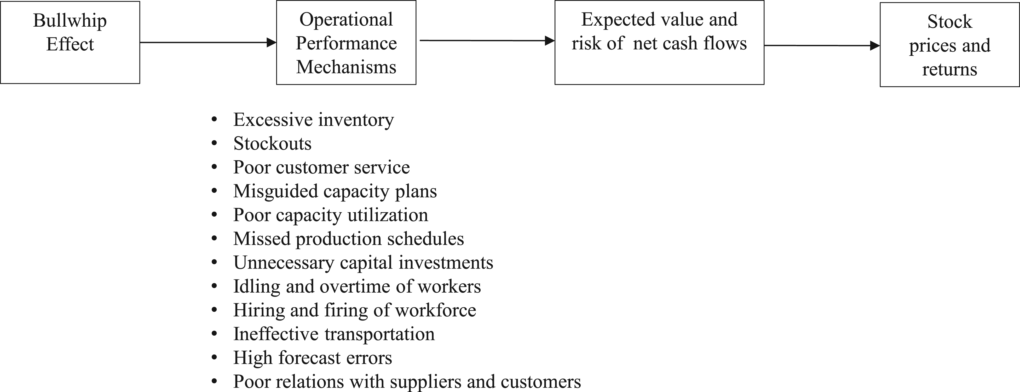
Link between the bullwhip effect (BWE) and stock returns.
Our analysis is based on data from 1985 to 2018 from about 7200 publicly traded firms on the New York, American, and NASDAQ stock exchanges. We measure the BWE using the amplification ratio (AR), as described in Cachon et al. (2007) and other empirical studies. Our results indicate no significant relationship between the BWE and stock returns. This is consistently observed for the full sample across all four approaches used to test the relationship and when we segment our sample by size, industry, and time periods. We also do not find a significant relationship between the BWE and stock returns for samples based on the propagation of AR from customers to suppliers. We do find some evidence to suggest that the BWE has a negative impact on inventory turnover. However, we do not see similar evidence for capacity utilization.
The remainder of the paper is organized as follows. The next section presents a conceptual model to develop the hypothesis on the link between the BWE and stock returns. Section 3 describes the data used, details on the construction of AR and the sorting of firms into five portfolios based on AR, and the estimation of stock returns of the portfolios. Section 4 presents the results on the relationship between ARs and stock returns of the 5 portfolios, and the results using the four-factor model as well as the Fama-MacBeth cross-sectional regressions. Section 5 considers the propagation of AR from customers to suppliers and its impact on stock returns. Section 6 presents the results on the effect of ARs on operational performance mechanisms (OPMs), such as inventory turnover and capacity utilization, and profitability. Section 7 summarizes the results and discusses the implications as well as possible future directions.
This section develops our primary hypothesis on the link between the BWE and stock returns. Figure 1 presents a conceptual model of the link between the BWE, OPMs, expected value and risk of net cash flows, and stock prices and returns. Figure 1 lists some commonly mentioned OPMs in the literature that are negatively impacted by the BWE (see, for example, Chatfield et al. (2004), Croson et al. (2014), Duan et al. (2015), Lee et al. (1997b), Metters (1997), and Wang and Disney (2016)). Analytical models show that the BWE can negatively impact inventory and stockouts (Tsay and Lovejoy (1999), Aviv (2007), and Chen and Lee (2012)). The negative impact of BWE on other OPMs is generally based on conceptual arguments on how the amplification of demand variability is detrimental. Using product and store-level data from a supermarket chain in China, Yao et al. (2021) find that higher BWE is associated with higher inventory and higher stockout rates. Beer Game experimental studies have observed that the BWE is associated with inventory levels 5 to 10 times greater than optimal levels (Sterman, 1989).
The negative impact of the BWE on OPMs can in turn negatively impact the expected value and risk of the net cash flows of a firm. On the revenue side, stockouts can lead to a loss in sales and market share, whereas excess inventory can lead to markdowns and loss of pricing power. Missed production schedules and poor customer service can lead to dissatisfaction and reduced loyalty among customers, and poor word-of-mouth, which can negatively impact revenues. Insufficient capacity and/or poor relations with suppliers may prevent the firm from capitalizing on strong market demand.
On the cost side, stockouts can increase backorder costs and penalties paid to customers. Excess inventories can increase the cost of holding inventory and can result in obsolete inventory that can require write-offs. The BWE can cause a firm with limited capacity to frequently adjust production levels that could require hiring or firing a workforce and/or shutting down and restarting facilities, which can increase costs. The increased volatility in production can affect the shipment and transportation capacity of the firm and can require the use of premium or expedited freight. The amplification of demand variability can also lead to non-optimal levels of investment in capacity.
The above discussion suggests that the BWE can have a negative impact on the expected net cash flows of the firm and increase the riskiness of the net cash flows. This can reduce the present value of cash flows because of lower expected cash flows as well as higher cost of capital due to increased riskiness of the cash flows. Since stock price reflects net cash flows, reductions in cash flows and/or increases in the risk of cash flows will have a negative impact on the stock prices and returns of the firm. Thus, our primary hypothesis is: H1: The BWE will have a negative effect on stock returns.
Measuring the BWE, Portfolio Formation Methodology, and Stock Returns
This section describes the data used in the empirical analysis. We discuss the measurement of the BWE and explain how this measure is used to form the BWE portfolios. We also discuss how we measure the stock returns of the BWE portfolios.
Measuring the BWE
There are two primary ways to measure the BWE. The first is the information flow bullwhip, which compares the variance of orders with the variance of demand. This measure reflects the original description of the BWE in Lee et al. (1997a). Although most analytical research uses the information flow bullwhip to measure the BWE, this measure is challenging to use for empirical research as information about orders and demand is generally not available. The second way to measure the BWE is the material flow bullwhip, which compares the variance of order receipts with the variance of sales. Cachon et al. (2007) argue that the variance of production is a good proxy for the variance of order receipts. Most empirical studies use the material flow bullwhip by comparing the variance of production with the variance of sales. Chen and Lee (2012) note that information flow bullwhip and material flow bullwhip measures are generally good approximations of each other. We use the material flow bullwhip to measure the firm-level BWE as:

To ensure fair comparison over time, COGS and inventory data are adjusted for inflation using deflator data from the Bureau of Economic Analysis. For firms in manufacturing and trade, we use implicit price deflators of their sectors (Bureau of Economic Analysis, 2018a). For all other firms, we use GDP deflator data (Bureau of Economic Analysis, 2018b).
We calculate production as

Cachon et al. (2007), Shan et al. (2014), and Osadchiy et al. (2021) find that both the production and the COGS time series are non-stationary because of a stochastic trend. In our sample, the Dickey-Fuller tests indicate that about 61% of the time series have a stochastic trend. Since the measure of BWE is based on variances, it is important to detrend the stochastic trend in the time series. The reason is that when a time series has a stochastic trend, its variance will depend on the length of the time horizon used to calculate the variances, which is undesirable. Differencing is the standard approach for detrending the stochastic trend. Accordingly, we detrend the series by taking the first log difference so that DPi,q (the detrended production in quarter q) = ln(Pi,q) – ln(Pi,q−1) and DCOGS i,q (the detrended COGS in quarter q) = ln(COGSi,q) – ln(COGSi,q−1). In our sample, about 12% of the difference time series are nonstationary.
AR is then measured as:

Summary statistics of amplification ratios (ARs) for the full sample and the four major industrial groups: mining, manufacturing, wholesale, and retail.
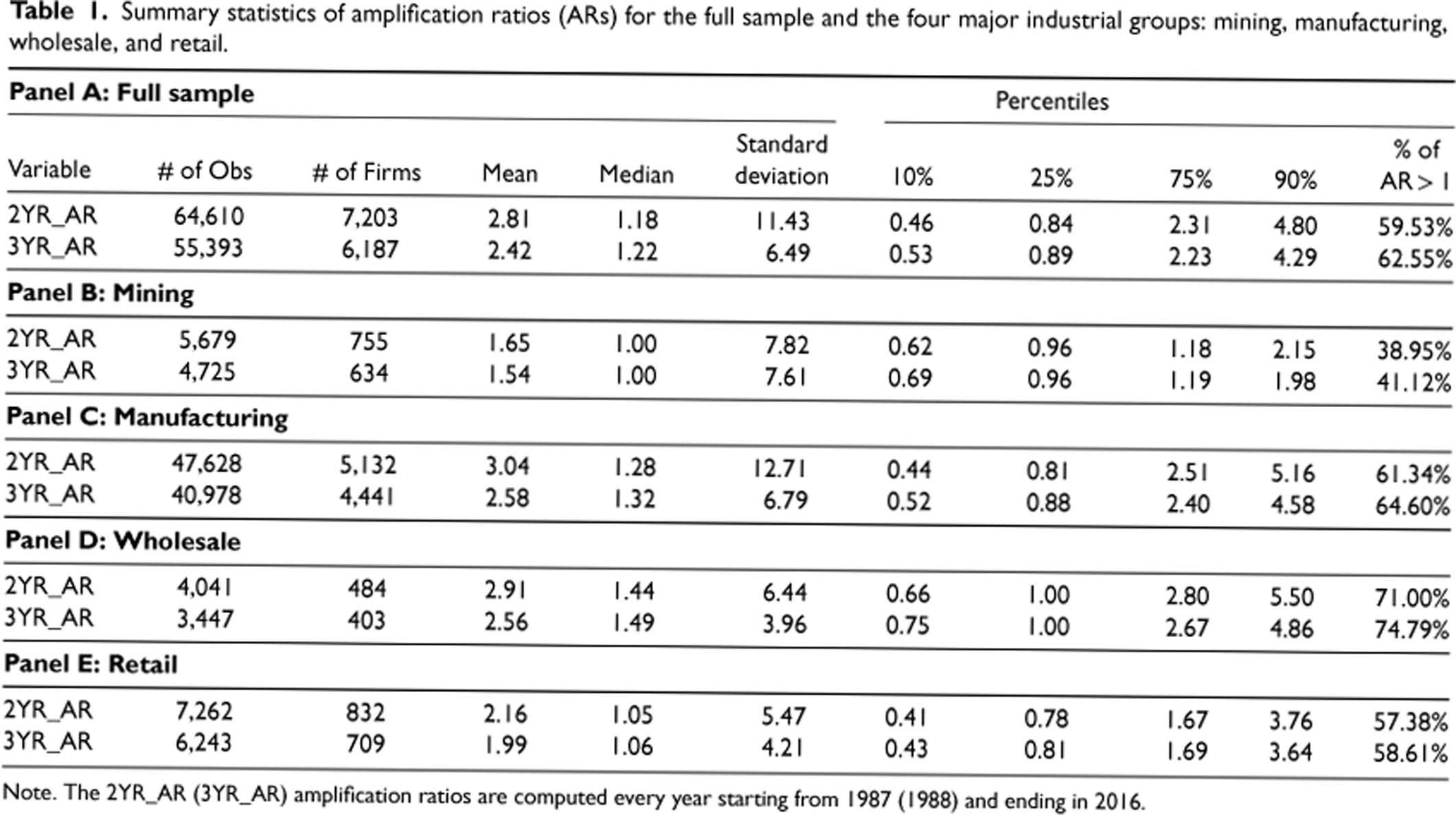
Note. The 2YR_AR (3YR_AR) amplification ratios are computed every year starting from 1987 (1988) and ending in 2016.
We calculate AR for each firm that reports quarterly accounting information for the fiscal quarter that falls in the last calendar quarter (October–December) of a year. We follow the approach of Osadchiy et al. (2021) who use 4, 8, and 12 quarters of data to estimate the BWE. Detailed results using 8 and 12 quarters of data are reported in Tables 1 to 4, and summary results using 4 quarters of data are reported in the robustness analysis of the portfolio results (Section 4.1.1).
We use the previous two years of detrended quarterly data to calculate AR (2YR_AR). Let q denote the fiscal quarter that falls in the last calendar quarter of a year. Then to calculate the 2YR_ARs, we use detrended data from fiscal quarters [q-7, q]. To calculate ARs, we require continuous data over [q-7, q] with no missing or nonpositive COGS data and no missing or negative inventory. We start estimating the 2YR_ARs from the fourth calendar quarter of 1987 and use a two-year rolling window to estimate ARs in every fourth calendar quarter through 2016.
We also use the previous three years’ detrended quarterly data to calculate the AR (3YR_AR). To calculate the 3YR_ARs, we use detrended data from quarters [q-11, q]. We start estimating the 3YR_ARs from the fourth calendar quarter of 1988 and use a three-year rolling window to estimate ARs in every fourth calendar quarter through 2016.
Table 1 reports the summary statistics for the ARs for the full sample as well as the four industrial groups: mining, manufacturing, wholesale, and retail. For the full sample, we have the 2YR_ARs for 64,610 firm-years from 7,203 distinct firms and the 3YR_ARs for 55,393 firm-years from 6,187 distinct firms. The mean (median) of the 2YR_ARs is 2.81 (1.18), and it is 2.42 (1.22) for the 3YR_ARs. The last column shows that the AR is greater than one for about 60% of the full sample. These statistics indicate that, on average, firms do bullwhip. This is consistent with the firm-level bullwhip results reported by Bray and Mendelson (2012) and Shan et al. (2014).
The industry-specific AR statistics indicate that about 40% of the firms in the mining industry bullwhip. Mining accounts for 10% of our sample. In manufacturing, which accounts for nearly 71% of our sample, the percentage of firms that bullwhip ranges from 61% to 64%, depending on whether we use the 2YR_ARs or the 3YR_ARs. The wholesale and retail sectors account for 7% and 12% of the sample, respectively. More than 70% of the firms in the wholesale sector bullwhip, whereas about 58% of the firms in the retail sector bullwhip. The results of Table 1 are consistent with the literature that the BWE is prevalent among firms, and it continues to persist.
Portfolios are a convenient way to statistically test whether the relationship between a variable and stock returns exists over a long time period. The basic idea is to construct portfolios by sorting on the variable of interest so that the constructed portfolios maximize the spread on the sorting variable, and thus the differences in the stock returns across the various portfolios can be attributed to the sorting variable. Fama and French (1993) and Carhart (1997) used the portfolio approach to identify size, growth, and momentum factors that are now common factors to explain the cross-section of stock returns. Other examples where the portfolio approach is used to examine the relation between specific variables and stock returns include inventory performance (Chen et al., 2005), media coverage (Fang and Peress, 2009), geographic dispersion of firms (Garcia and Norli, 2012), inventory turnover of retailers (Alan et al. 2014), 8-k filings (Zhao, 2017), investor overconfidence (Adebambo and Yan, 2018), default risk (Aretz et al., 2018), and extent of global sourcing (Jain and Wu, 2023), among others.
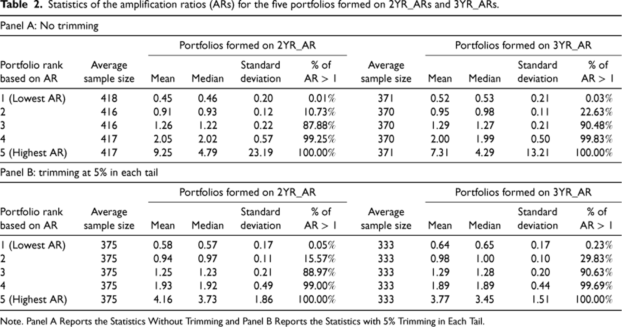
Statistics of the amplification ratios (ARs) for the five portfolios formed on 2YR_ARs and 3YR_ARs.
Statistics of the amplification ratios (ARs) for the five portfolios formed on 2YR_ARs and 3YR_ARs.
Note. Panel A Reports the Statistics Without Trimming and Panel B Reports the Statistics with 5% Trimming in Each Tail.
To investigate the relation between AR and stock returns, we follow Fama and French (1993) to form portfolios based on the 2YR_ARs and the 3YR_ARs. On June 30 of each year t we form five portfolios using all the firms for which we could compute the ARs in the last calendar quarter (October–December) of year t − 1. For example, on June 30, 2010, we form the portfolios using firms whose ARs were calculated in October–December of 2009. To ensure a balanced industry representation across the portfolios, we rank firms in each of the two-digit SIC codes in ascending order of AR and divide these firms into five quintiles. Firms in the lowest quintile of ARs comprise Portfolio 1, while firms in the highest quintile of ARs comprise Portfolio 5. We then aggregate the firms from the various two-digit SIC codes for each quintile portfolio, to get the five portfolios for year t. We liquidate these portfolios and form new portfolios on June 30 of year t + 1 using ARs computed in the last calendar quarter of year t. In other words, the portfolios are updated annually. Using the 2YR_ARs, we form the first portfolios on June 30, 1988, and the last on June 30, 2017 (30 years). In the case of the 3YR_ARs, the first portfolios are formed on June 30, 1989, and the last on June 30, 2017 (29 years).
Panel A of Table 2 reports the AR statistics for the 2YR_ARs and the 3YR_ARs for the five portfolios formed by sorting ARs across all years. Note that the lowest AR firms are in Portfolio 1 and the highest AR firms are in Portfolio 5. Over 30 (29) years, the mean number of firms in each portfolio based on the 2YR_ARs (3YR_ARs) is about 417 (370). The spread in the level of ARs across the lowest and highest AR portfolios is high. For the portfolios based on sorting on the 2YR_ARs, the mean (median) AR of the lowest AR portfolio (Portfolio 1) is 0.45 (0.46) and is 9.25 (4.79) for the highest AR portfolio (Portfolio 5). Nearly all firms in the lowest AR portfolio do not bullwhip (AR < 1), whereas all firms in the highest AR portfolio bullwhip (AR > 1). The spread between Portfolios 2 and 4 is also high, with the mean and median of Portfolio 2 about half that of Portfolio 4. Nearly 90% of the firms in Portfolio 2 do not bullwhip, whereas nearly all the firms in Portfolio 4 bullwhip. The mean (median) AR of Portfolio 3 is 1.26 (1.22) and about 88% of the firms in this portfolio bullwhip. Overall, most of the firms in Portfolios 1 and 2 do not bullwhip, whereas most of the firms in Portfolios 3, 4, and 5 bullwhip. The results are similar for portfolios based on the 3YR_ARs.
The mean and standard deviation of Portfolio 5 are high because some firms with large ARs get assigned to Portfolio 5, given our sorting approach. This should not be of concern in testing the relationship between the BWE and stock returns as we estimate the stock returns at the portfolio level weighted by market value, and thus a few outlier firms with high ARs will not drive the portfolio returns. Nonetheless, to address any issue that can arise from including these high AR firms, we also create portfolios after trimming ARs at the 5% level in each tail in each of the two-digit SIC codes. Panel B of Table 2 reports the AR statistics of the trimmed sample. The mean and standard deviation of Portfolio 5 are much lower under the trimmed sample when compared to the sample without trimming (Panel A).
Panel A reports the sample statistics for the five portfolios formed on 2YR_ARs. Panel B reports the sample statistics for the five portfolios formed on 3YR_ARs. Panel C reports the transition frequencies between portfolios from one year to the next year.
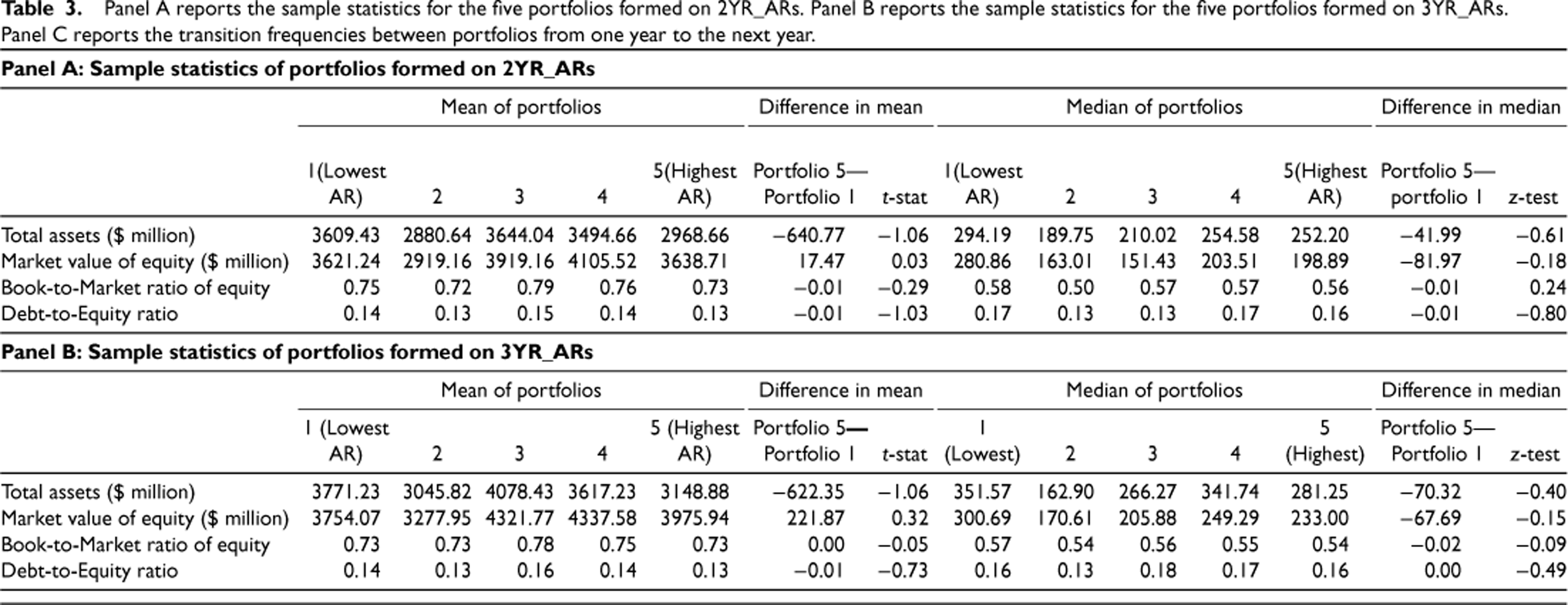
Panel A of Table 3 reports the summary statistics of selected firm characteristics across all years for the AR portfolios based on the 2YR_ARs and the 3YR_ARs. The characteristics reported are total assets, market value of equity, book-to-market ratio of equity (the ratio of the book value of equity to the market value of equity), and debt-to-equity ratio (the ratio of the book value of debt to the sum of the book value of debt and the market value of equity). The results indicate that the mean and the median of the characteristics for the two extreme AR portfolios (Portfolio 1 and Portfolio 5) are similar, and the differences are not statistically significant. Furthermore, our method of forming portfolios ensures that the distributions of the two-digit SIC codes are similar across the portfolios.
On a year-to-year basis, we can expect some stability in the assignment of firms to the quintile portfolios. There are two reasons for this. First, firms are unlikely to change production policies significantly on a year-to-year basis, as implementing significant changes can be time-consuming and expensive. Second, data from overlapping quarters are used to construct the ARs for any two consecutive years. For example, the data overlap is 4 out of 8 quarters for the 2YR_ARs, and the data overlap is 8 out of 12 quarters for the 3YR_ARs. To get an idea about stability in the assignment of firms to the quintile portfolios, we estimate a transition matrix that measures the propensity that a firm in any portfolio in any year to remain in the same portfolio next year or switch to another portfolio next year.
Panel C of Table 3 shows that for the portfolios based on the 2YR_ARs, about 61% of the firms that are in Portfolio 1 in year t remain in Portfolio 1 in year t + 1. About 17%, 10%, 8%, and 4% of the firms in Portfolio 1 in year t transition to Portfolios 2, 3, 4, and 5, respectively, in year t + 1. In the case of Portfolio 5, about 60% of the firms that are in Portfolio 5 in year t remain in Portfolio 5 in year t + 1. About 22%, 8%, 5%, and 5% of the firms in Portfolio 5 of year t transition to Portfolios 4, 3, 2, and 1, respectively, in year t + 1. In the case of the 3YR_ARs, about 71% (69%) of the firms that are in Portfolio 1 (Portfolio 5) in year t remain in Portfolio 1 (Portfolio 5) in year t + 1. The transition matrices indicate that about 80% of the firms remain either in the same portfolio or in an adjacent portfolio from one year to the next and are less likely to jump more than one portfolio.
Once the portfolios for year t are formed, we track value-weighted returns for each portfolio from July of year t to June of year t + 1. In calculating the value-weighted portfolio returns, the firms are weighted by the market value of equity at the end of June of year t. Since the portfolios are updated on June 30 of each year, we repeat the tracking of monthly returns on an annual basis. For example, the first set of portfolios using the 2YR_ARs are formed on June 30, 1988, and monthly returns for these portfolios are tracked from July 1, 1988 to June 30, 1989. The last set of portfolios using the 2YR_ARs is formed on June 30, 2017, and monthly returns for these portfolios are tracked from July 1, 2017 to June 30, 2018. Using the 2YR_ARs (3YR_ARs) to form the portfolio results in a time series of 360 (348) monthly returns from July 1988 to June 2018 (July 1989 to June 2018) for each portfolio. Monthly returns are from the Center of Research in Security Prices. If a firm's monthly return is missing, we set the missing return equal to the value-weighted market return.
AR Portfolios and Stock Returns
This section reports the mean monthly returns for the five portfolios. For the portfolios based on the 2YR_ARs (3YR_ARs), the mean monthly returns are the mean over 360 (348) monthly returns from July 1988 to June 2018 (July 1989 to June 2018). The results are reported for the full sample as well as the subsamples of size, industry, and time periods. Our hypothesis is that BWE will have a negative impact on stock returns. Thus, one would expect that high bullwhip firms (Portfolio 5) will have lower stock returns than low bullwhip firms (Portfolio 1) and the difference between the returns of Portfolios 5 and 1 will be negative. This is the same as adopting a long-short investment strategy that is long on (buys) Portfolio 5 (the highest AR portfolio) and short on (sells) Portfolio 1 (the lowest AR portfolio). If BWE has a negative impact on stock returns, one would expect the stock returns to increase as we move from Portfolio 5 to Portfolio 1, and the stock returns of the long-short portfolio would be negative.
Portfolio Results for the Full Sample
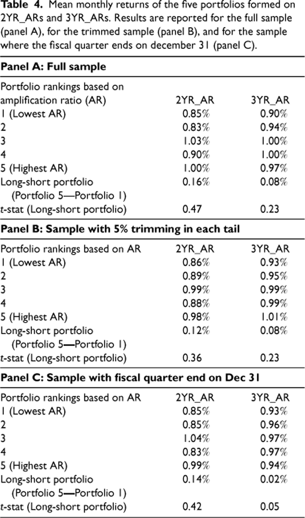
Panel A of Table 4 reports the returns for the five AR portfolios. Focusing on the returns for the portfolios formed using the 2YR_ARs, the mean monthly return of the highest AR firms (Portfolio 5) is 1.00%. As we move from Portfolio 5 to Portfolio 1, AR decreases, but the returns show no specific pattern. For example, the returns for the lowest AR firms (Portfolio 1) is 0.85%, but it is lower than the returns for Portfolios 3 and 4. The return on Portfolio 4 is also lower than the return on Portfolio 5. The long-short portfolio that buys Portfolio 5 and sells Portfolio 1 yields returns of 0.16% per month, statistically indistinguishable from zero. The results are similar when the portfolios are formed using the 3YR_ARs.
Mean monthly returns of the five portfolios formed on 2YR_ARs and 3YR_ARs. Results are reported for the full sample (panel A), for the trimmed sample (panel B), and for the sample where the fiscal quarter ends on december 31 (panel C).
Mean monthly returns of the five portfolios formed on 2YR_ARs and 3YR_ARs. Results are reported for the full sample (panel A), for the trimmed sample (panel B), and for the sample where the fiscal quarter ends on december 31 (panel C).
In untabulated results, we also form a long-short portfolio that buys all the firms that bullwhip (AR > 1) and sells all the firms that do not bullwhip (AR <1). The mean monthly return of this portfolio is statistically indistinguishable from zero.
Panel B of Table 4 reports the returns when the portfolios are formed after trimming ARs at the 5% level in each tail in each of the two-digit SIC codes. This eliminates firms with very low and very high ARs from being included in the portfolios. The mean number of firms in each portfolio based on the 2YR_ARs (3YR_ARs) is about 375 (333). For the portfolio returns formed using the 2YR_ARs, the mean monthly return of the highest AR firms (Portfolio 5) is 0.98% and it is 0.86% for the lowest AR firms (Portfolio 1). The mean monthly return of 0.12% on the long-short portfolio strategy that buys Portfolio 5 and sells Portfolio 1 is statistically indistinguishable from zero. The results are similar when the portfolios are formed using the 3YR_ARs.
To ensure that ARs are known before the returns they are used to are estimated, we use quarterly accounting information for the fiscal quarter that falls in the last calendar quarter (October–December) of year t-1 to create the portfolio on June 30 of year t, and then track the returns from July of year t to June of year t + 1. Thus, there is a gap between the fiscal quarter end when AR is measured and when we start tracking the returns. Such gaps are normal in studies that use the portfolio approach (see, for example, Fama and French (1993)). In our analysis, this gap could range from 6 to 9 months. To test if this variation in gap affects the results, we estimate the returns for the subsample of firms whose fiscal quarter ends specifically on December 31 (rather than on any date in the fourth quarter). This ensures that all firms have the same gap of 6 months.
Nearly 80% of our sample firms have a fiscal quarter that ends on December 31. Panel C of Table 4 reports the results for this subsample. These results are very similar to those for the full sample. The mean monthly return of 0.14% on the long-short portfolio is statistically indistinguishable from zero. The results are similar when the portfolios are formed using the 3YR_ARs.
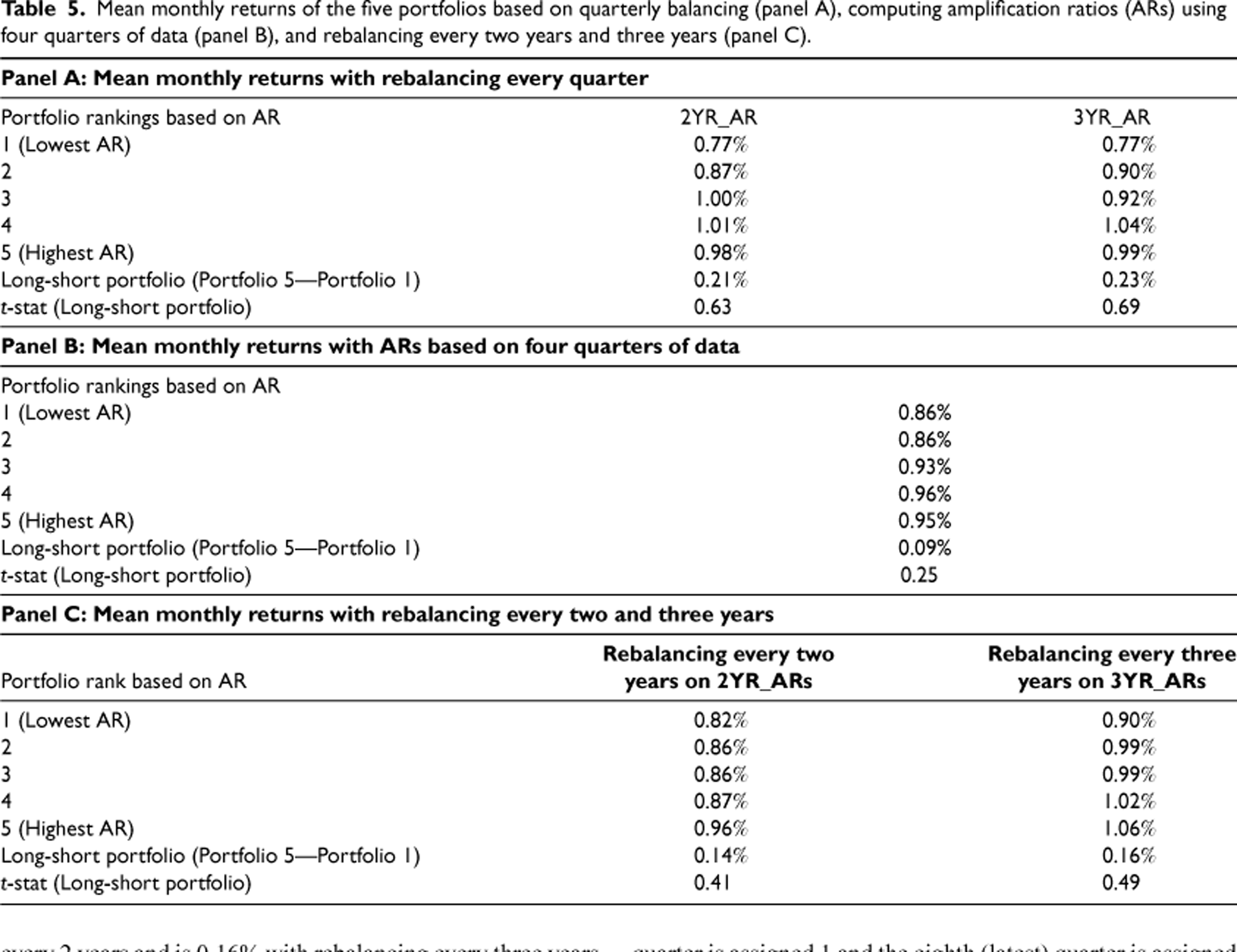
The results reported in Table 4 are based on calculating ARs annually using data for the quarter that ended in October to December of each year. These ARs are used to rebalance the portfolio on June 30 next year. We reran our results by updating ARs more frequently and rebalancing the portfolios three months after updating the ARs. ARs are updated quarterly with quarters ending in January–March, April–June, July–September, and October–December. Portfolios are liquidated and reinvested three months after the quarter when the ARs are updated. For example, for the ARs calculated for quarters ending in January-March, portfolios are liquidated and reinvested on June 30, for the ARs calculated for quarters ending in April-June, portfolios are liquidated and reinvested on September 30, and so on.
Panel A of Table 5 reports these results for the five AR portfolios. Focusing on the 2YR_ARs results, the mean monthly return for the highest AR firms (Portfolio 5) is 0.98% and is 0.77% for the lowest AR firms (Portfolio 1). The long-short portfolio that buys Portfolio 5 and sells Portfolio 1 yields returns of 0.21% per month, statistically indistinguishable from zero. The results are similar for the 3YR_ARs.
Mean monthly returns of the five portfolios based on quarterly balancing (panel A), computing amplification ratios (ARs) using four quarters of data (panel B), and rebalancing every two years and three years (panel C).
Mean monthly returns of the five portfolios based on quarterly balancing (panel A), computing amplification ratios (ARs) using four quarters of data (panel B), and rebalancing every two years and three years (panel C).
Since the results presented in Table 4 are based on the annual rebalancing of the portfolios, we expect some stability in the portfolio membership because of the overlapping quarters used in constructing the AR measure for any two consecutive years. To see if this overlap affects the results, we did two additional tests. First, to avoid any overlap, we compute the 1YR_ARs using four quarters of non-overlapping data. Panel B of Table 5 reports the results for the five AR portfolios. As we move from Portfolio 5 to Portfolio 1, AR decreases but the returns show no specific pattern. The mean monthly return for the highest AR firms (Portfolio 5) is 0.95% and 0.86% for the lowest AR firms (Portfolio 1). The long-short portfolio that buys Portfolio 5 and sells Portfolio 1 yields returns of 0.09% per month, statistically indistinguishable from zero.
Second, instead of rebalancing every year, we rebalance every 2 years (3 years) when portfolios are formed using the 2YR_ARs (3YR_ARs). We then track the monthly returns for 24 months (36 months) for the portfolios based on the 2YR_ARs (3YR_ARs) and rebalance the portfolios every two years (three years). Panel C of Table 5 reports these results. The mean monthly return on the long-short portfolio that buys Portfolio 5 and sells Portfolio 1 is 0.14% with rebalancing every 2 years and is 0.16% with rebalancing every three years. Both returns are statistically indistinguishable from zero.
In the E-companion, we report the stock returns for AR portfolios on the subsamples of small, medium, and large firms; four different industry groups, and three different time periods. Overall, the results indicate that there is no difference in the stock returns of high AR portfolios and low AR portfolios across these subsamples. We also run all the above analyses using equally weighted portfolio returns. The results are similar to those from value-weighted returns.
The results reported in Table 4 are based on computing ARs by equally weighting each quarter. An issue with using equal weights over 8 or 12 quarters data is that the variations in production and sales are averaged over 2 or 3 years, which might make the portfolios somewhat stable. To test whether this affects the results, we use the weighted variance approach to estimate the ARs where more (less) weight is given to recent (earlier) quarters. We calculate the weighted variance in two ways.
The first way assigns a number to each quarter and uses these numbers to compute the weights for each quarter. To illustrate, when we use 8 quarters of data, we assign a number from 1 through 8 to the eight quarters where the first (earliest) quarter is assigned 1 and the eighth (latest) quarter is assigned 8. We calculate the weights by dividing these numbers by 36 where 36 is the sum of the numbers 1 through 8. The first quarter is assigned a weight of 1/36, the quarter after that is assigned a weight of 2/36, and so on, and the eighth quarter is assigned a weight of 8/36. We use a similar approach with 12 quarters of data where the numbers range from 1 to 12, and the weights are calculated by dividing the numbers by 78. We call this method linear weights.
The second approach uses an exponential growth function with growth rates of 10% and 20% to calculate the weights. To illustrate, for 10% growth with 8 quarters of data, we assign 1 to the first quarter, 1.1 to the second quarter, 1.21 to the third quarter, and so on, with 1.95 (1.1∧7) to the eighth quarter. These numbers are then used to calculate the weights for each quarter. For the 10% growth with 12 quarters of data we assign 1 to the first quarter, 1.1 to the second quarter, 1.21 to the third quarter, and so on, with 2.85 (1.1∧11) to the twelfth quarter. Table 6 presents these results.
Mean monthly returns of the five portfolios formed on 2YR_ARs and 3YR_ARs.
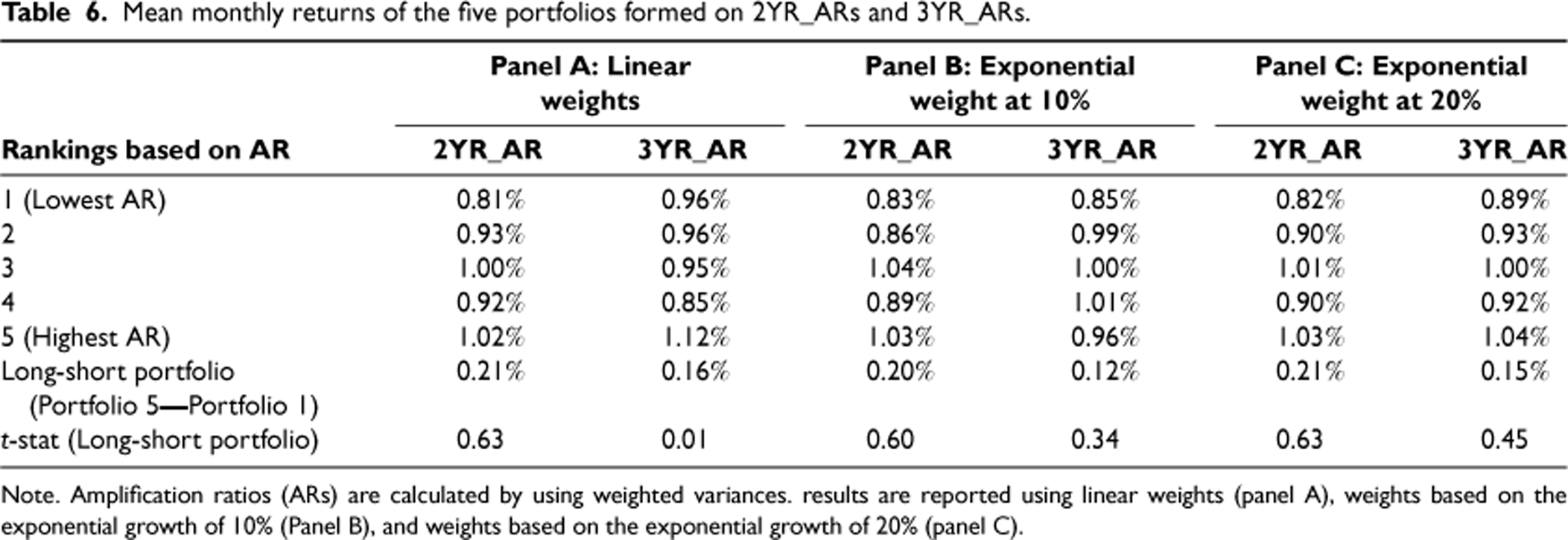
Note. Amplification ratios (ARs) are calculated by using weighted variances. results are reported using linear weights (panel A), weights based on the exponential growth of 10% (Panel B), and weights based on the exponential growth of 20% (panel C).
Focusing on the 2YR_ARs results in Panel A, the mean monthly return of the highest AR firms (Portfolio 5) is 1.02% and is 0.81% for the lowest AR firms (Portfolio 1). The long-short portfolio that buys Portfolio 5 and sells Portfolio 1 yields returns of 0.21% per month, statistically indistinguishable from zero. The results are similar for 3YR_ARs and when weights are based on exponential growth of 10% and 20%.
The results on the relationship between ARs and stock returns presented in the previous section are based on the univariate analysis of raw returns. A concern with univariate analyses is that we have not controlled for other factors that affect stock returns. To test whether our univariate results hold in a multivariate analysis, we use two approaches commonly employed in the literature. The first approach is a time-series multivariate test based on the four-factor asset pricing model (Fama and French, 1993, and Carhart, 1997). The second approach is a cross-sectional multivariate test based on the Fama-MacBeth (1973) regressions. Some recent papers where these approaches are used include Alan et al. (2014), Zhao (2017), Adedambo and Yan (2018), Aretz et al. (2018), and Jain and Wu (2023), among others. We next describe and present the results from these two approaches.
Results from the Four-Factor Model
The four-factor model posits that the return on an asset is a linear function of four factors. The four-factor model is estimated using the following regression:

The interpretation of
Table 7 presents the regression results from the four-factor model for the five portfolios and the long-short portfolio based on the 2YR_ARs and the 3YR_ARs. Each regression is based on the time series of the mean monthly returns of the respective portfolio over 360 months (July 1988 to June 2018) using 2YR_ARs, and 348 months (July 1989 to June 2018) using 3YR_ARs.
Regression results for the four-factor model for the five portfolios formed on 2YR_ARs and 3YR_ARs.
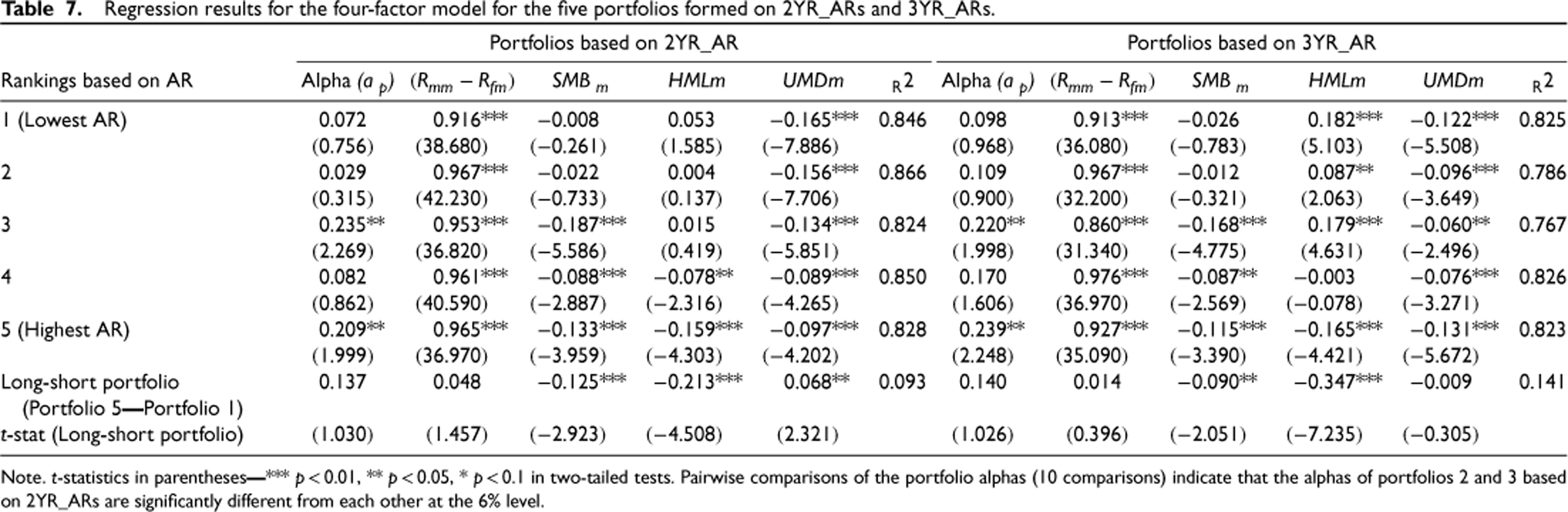
Note. t-statistics in parentheses
The four-factor regressions of portfolios based on the 2YR_ARs indicate that the coefficients of
In untabulated results, we estimate the four-factor regressions on the subsamples of small, medium, and large firms, four different industry groups, and three different time periods. For each of these 10 subsamples, we estimate
In this section, we use a cross-sectional asset return model to examine the relationship between AR and stock returns. More specifically, we perform the Fama and MacBeth (1973) cross-sectional regressions using monthly returns. For each month in our sample period, we regress each firm's monthly stock returns on AR and other variables that are commonly known to influence stock returns. For example, using the 2YR_ARs, the sample period spans July 1988 through June 2018, or 360 months. We run 360 regressions for each month from July 1988 through June 2018 to generate a time series of 360 regression coefficients for each variable. We estimate the effect of each variable on stock returns by the mean of the time series of its regression coefficients. Statistical significance for the mean coefficient of each variable is calculated using the standard error of the time series of its regression coefficient.
For each month m in our sample period, we run the following regression:

We note that size, beta, book-to-market ratio of equity, and the returns of the firm in the previous 12 months are commonly used in Fama-MacBeth regressions (see, for example, Alan et al. (2014), Zhao (2017), Adedambo and Yan (2018), and Aretz et al. (2018)). In running the regressions for month m, we only include firms that have information on all the above variables in month m.
The variable of interest in the Fama-MacBeth regression is AR. If the BWE has a negative impact on stock returns, then the coefficient of AR should be negative. Table 8 presents the results for four different models of Fama-MacBeth regressions using the 2YR_ARs and the 3YR_ARs. The difference across the models is in the operationalization of ARs. In Model 1 we use the actual AR values for each firm. The coefficient of AR in Model 1 is 0.005% based on the 2YR_Ars, and it is 0.006% based on the 3YR_ARs. The coefficients of AR imply that a unit increase in AR increases the stock returns by 0.005% or 0.006%, which is small and not economically significant. Note that only the coefficient of AR based on the 2YR_ARs is marginally significant at the 10% level in a two-tailed test.
Results of the Fama-Macbeth regression results.
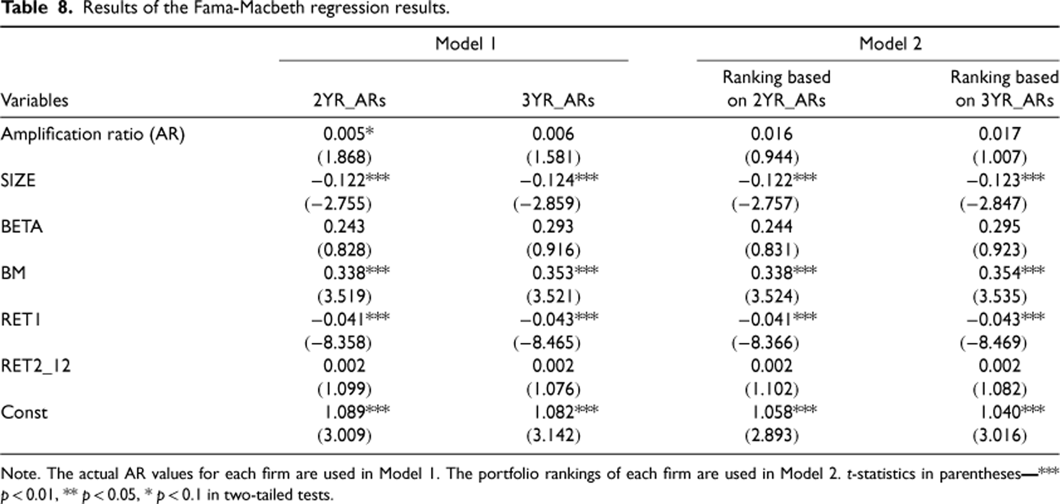
Note. The actual AR values for each firm are used in Model 1. The portfolio rankings of each firm are used in Model 2. t-statistics in parentheses
The positive relationship between AR and stock returns in Model 1 is not robust when alternate specifications of ARs are used. In Model 2, instead of using the actual AR values of each firm, we use the portfolio rankings of each firm based on the portfolio formation method described in Section 2. Recall that the lowest (highest) AR firms are in Portfolio 1 (Portfolio 5). The use of portfolio rankings allows for nonlinearity and can mitigate the effect of extreme observations in estimating coefficients (Alan et al., 2014). The coefficients of AR in Model 2 are positive but statistically indistinguishable from zero.
In untabulated results, we estimate the Fama-MacBeth regressions for the subsamples of small, medium, and large firms, four different industry groups, and three different time periods. For each of these 10 subsamples, we estimate the AR coefficients using the actual AR values for each firm and the portfolio rankings of each firm from the 2YR_ARs and the 3YR_ARs. Only the AR coefficients of the subsample of large firms are positive and significant in Model 2 where ARs are measured using the portfolio rankings of each firm. However, this result is not robust to alternate specifications of ARs. When actual values of AR are used, the AR coefficients for the subsample of large firms are positive but statistically indistinguishable from zero.
In the E-companion, we report the stock return results using the moving range portfolio approach of Chen et al. (2007). These results are consistent with the results presented in this section. Overall, we do not find evidence of a consistent significant relationship between ARs and stock returns.
The results in Section 4 are based on the ARs at the firm level that captures the demand distortion at the firm level. It does not consider how the demand distortion propagates up the supply chain, which is an important aspect of the BWE. This section extends our analysis to consider the propagation of AR from customers to suppliers. We use the idea of Mackelprang and Malhotra (2015), who measure changes in the AR from customer to supplier and use this to examine the profitability impact on suppliers. In other words, they attempt to capture how the demand distortion propagates upstream and whether it is amplified or dampened. For example, given the AR of a customer, the supplier's AR may be higher (amplification) or lower (dampened) than the customer's AR. We use supply chain network data to create customer-supplier dyads and examine whether the relationships between customer AR and supplier AR affect the stock returns.
Mean monthly returns of the five portfolios formed on 2YR_ARs and 3YR_ARs.
Mean monthly returns of the five portfolios formed on 2YR_ARs and 3YR_ARs.
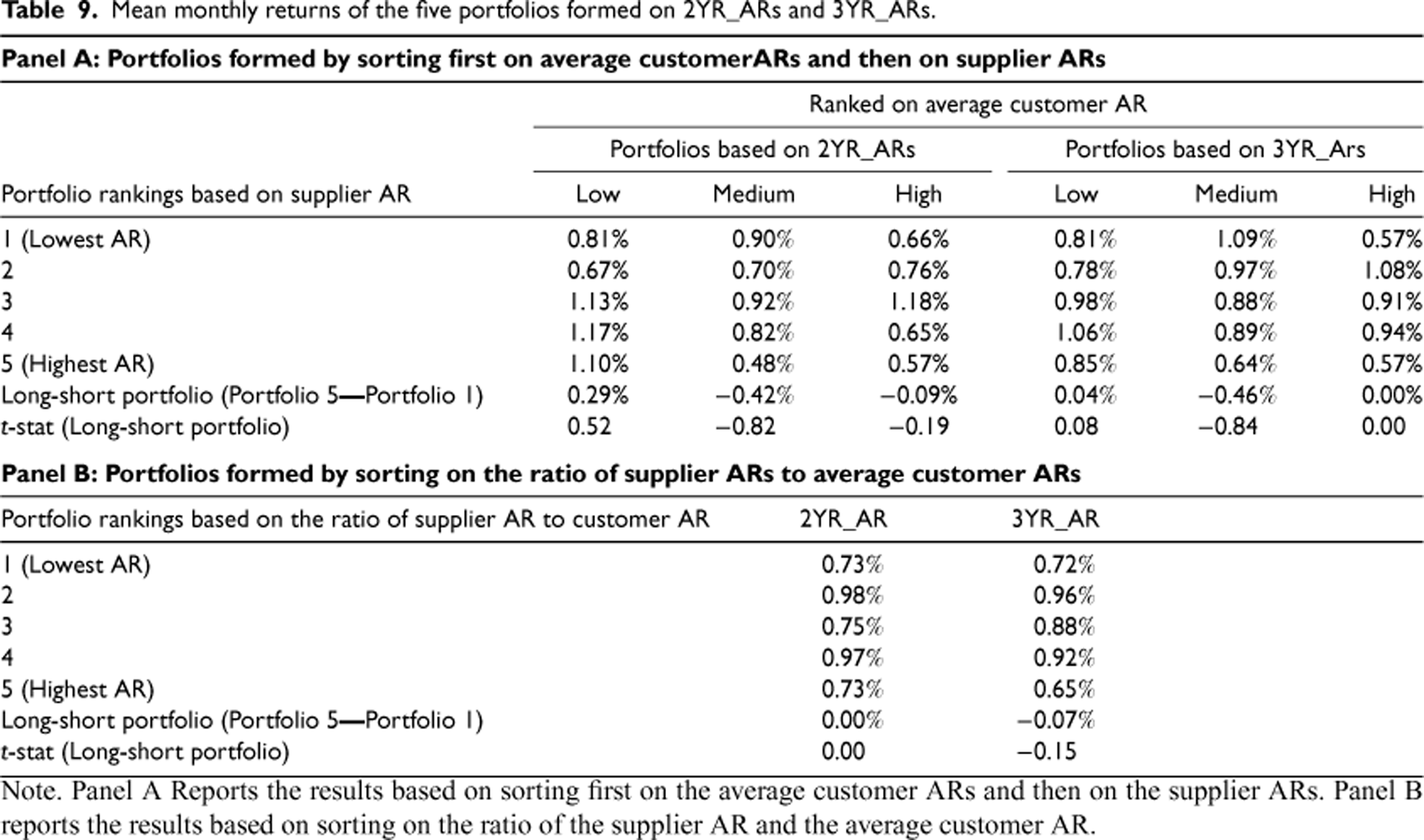
Note. Panel A Reports the results based on sorting first on the average customer ARs and then on the supplier ARs. Panel B reports the results based on sorting on the ratio of the supplier AR and the average customer AR.
We use the supply chain network data from the FactSet Revere database to create customer-supplier dyads. The dataset collects supply chain relationship information from corporate financial statements, investor presentations, press releases, etc. It covers more than 10,000 public firms globally and reports about 25,000 customer-supplier relationships annually. For each customer-supplier relationship, FactSet Revere reports the start and end dates of the relationship. The dataset reports customer-supplier relationship information starting in 2003. Baron et al. (2023) also use this dataset to classify their sample firms as suppliers or customers of Japanese firms to analyze the financial consequences of the BWE from the Fukushima disaster of March 11, 2011.
Consistent with our analyses of the BWE at the firm level, we restrict the supply chain network data to those firms that are covered in FactSet Revere and are in the following two-digit SIC codes: Mining (SIC 10–14), manufacturing (SIC 20–39), wholesale (SIC 50–51) and retail (SIC 52–59). For each supplier, the customer-supplier dyad consists of the supplier and all its customers. For each customer-supplier dyad, we compute the 2YR_AR and 3YR_AR of the supplier and the average 2YR_AR and 3YR_AR of all its customers. Thus, for each customer-supplier dyad, we have the average customer AR and the supplier AR.
Restricting the sample to suppliers with information about customers in the FactSet Revere database does reduce the sample size. For example, the results in Sections 3 and 4 are based on an average of 2,000 firms per year from 1987 to 2016. In contrast, the results using the supply chain network data from the FactSet Revere database are based on an average of about 1,200 firms per year from 2003 to 2016. We note that Mackelprang and Malhotra (2015) use the Compustat data, which collects supply chain only from the financial statements, to construct supplier-customer dyads but only focus on those dyads where the customers collectively account for at least 50% of the supplier's sales. This severely restricts their sample size. Their analysis is based on a sample of 383 firms over 18 years or about 21 firms per year.
To examine how the propagation of demand distortion from customers to suppliers affects suppliers’ stock returns, we sort first on average customer ARs and then on supplier ARs. On June 30 of each year t for each two-digit SIC code, we sort the customer ARs into low, medium, and high subsamples using terciles of customer ARs as cut-offs. On average, each of the three subsamples has about 400 firms. The mean AR of the low, medium, and high customer AR subsamples is 0.89, 1.71, and 5.88, respectively. Each of the three customer AR subsamples at the two-digit SIC code level is sorted into quintiles based on the supplier AR. We then aggregate the firms from the various two-digit SIC codes across the three customer AR subsamples to create 15 customer-supplier AR portfolios for year t. The spread in the mean level of supplier AR across the lowest and highest AR portfolios is 0.41 to 7.76 for the low customer AR subsample, 0.49 to 10.79 for the medium customer AR subsample, and 0.52 to 10.4 for the large customer AR subsample.
Panel A of Table 9 reports the mean monthly returns of the customer-supplier AR portfolios. Focusing on the 2YR_AR returns for low customer AR firms, the mean monthly return for the highest AR suppliers (Portfolio 5) is 1.10% and is 0.81% for the lowest AR suppliers (Portfolio 1). The mean monthly return of 0.29% on the long-short portfolio strategy that buys Portfolio 5 and sells Portfolio 1 is statistically indistinguishable from zero. The long-short portfolio mean monthly return for medium customer AR firms is −0.42%, and for large customer AR firms, it is −0.09%; both are statistically indistinguishable from zero. The results are similar when the portfolios are formed using the 3YR_ARs. To explore if these insignificant results persist across the supply chain, we repeat the analysis of Panel A of Table 9 for the subsample where the customer is only from the retail sector (two-digit SIC 52–59). These results, reported in the E-companion, are statistically indistinguishable from zero.
We also conduct the analysis by creating portfolios using the ratio of the supplier AR and the average customer AR. This ratio measures the extent of amplification or dampening from customer to supplier. On June 30 of each year t, we rank firms in each of the two-digit SIC codes in ascending order of this ratio and divide these firms into five quintiles. We then aggregate the firms from the various two-digit SIC codes for each quintile portfolio, to get the five portfolios for year t. Based on an average sample of 1,200 observations per year from 2003 to 2016, the mean (median) ratio is 1.89 (0.81). On average, suppliers in Portfolios 1, 2, and 3 do not amplify the customer AR (average ratio is < 1) whereas suppliers in Portfolios 4 and 5 amplify the customer AR (average ratio is > 1).
Panel B of Table 9 reports the returns for the five portfolios formed based on the ratio of supplier AR to customer AR. Focusing on the returns for the portfolios formed using the 2YR_ARs, the mean monthly return of the highest AR firms (Portfolio 5) is 0.73% and is also 0.73% for the lowest AR suppliers (Portfolio 1). The mean monthly return on the long-short portfolio strategy that buys Portfolio 5 and sells Portfolio 1 is statistically indistinguishable from zero. The results are similar when the portfolios are formed using the 3YR_ARs.
In the E-companion, we report the results of the customer-supplier dyad analysis using supply chain network data from Compustat. Compustat has a longer history of reporting customer information than the FactSet Revere database. However, the information reported in Compustat is based on Regulation SFAS No. 1311, which requires that the US publicly traded firms disclose their customers that account for more than 10% of their annual sales. The 2YR_ARs (3YR_ARs) results are based on an average of 404 (355) firms per year from 1987 to 2016. These results are similar to the results based on the FactSet Revere database.
Overall, the results indicate that considering customer ARs together with supplier ARs still shows that the impact of the BWE on stock returns is statistically indistinguishable from zero.
Relationship Between ARs and OPMs
In Section 2, we discussed that the link between the BWE and stock returns is through OPMs (see Figure 1). Our results indicate that the impact of the BWE on stock returns is statistically indistinguishable from zero. To further explore this, we examine the link between the BWE and OPMs by considering inventory turnover and capacity utilization. These are two of the commonly mentioned OPMs in the BWE literature, and data to measure these is publicly available. We measure inventory turnover as the ratio of the annual COGS and the average of the start of the year and end of the year total inventory. Following Hendricks et al. (2009), we measure annual capacity utilization as the ratio of annual production and the average of the start of the year and end of the year net property, plant, and equipment.
To test for the link between BWE and inventory turnover and capacity utilization, we sort firms on June 30 of each year t into five portfolios based on the AR as we did for the stock returns analyses, and then compare the inventory turnover and capacity utilization performance across portfolios. Given that the BWE can have a negative impact on inventory turnover and capacity utilization, one would expect a monotonic decrease in inventory turnover and capacity utilization as one moves from the lowest AR portfolio (Portfolio 1) to the highest AR portfolio (Portfolio 5). Inventory turnover and capacity utilization are measured at the end of the fiscal year that ends after the portfolio formulation date. Table 10 presents these results for the portfolios based on the 2YR_ARs and the 3YR_ARs. Since the mean value of OPMs can be affected by outliers, the means are reported after winsorizing at the 2.5% level in each tail.
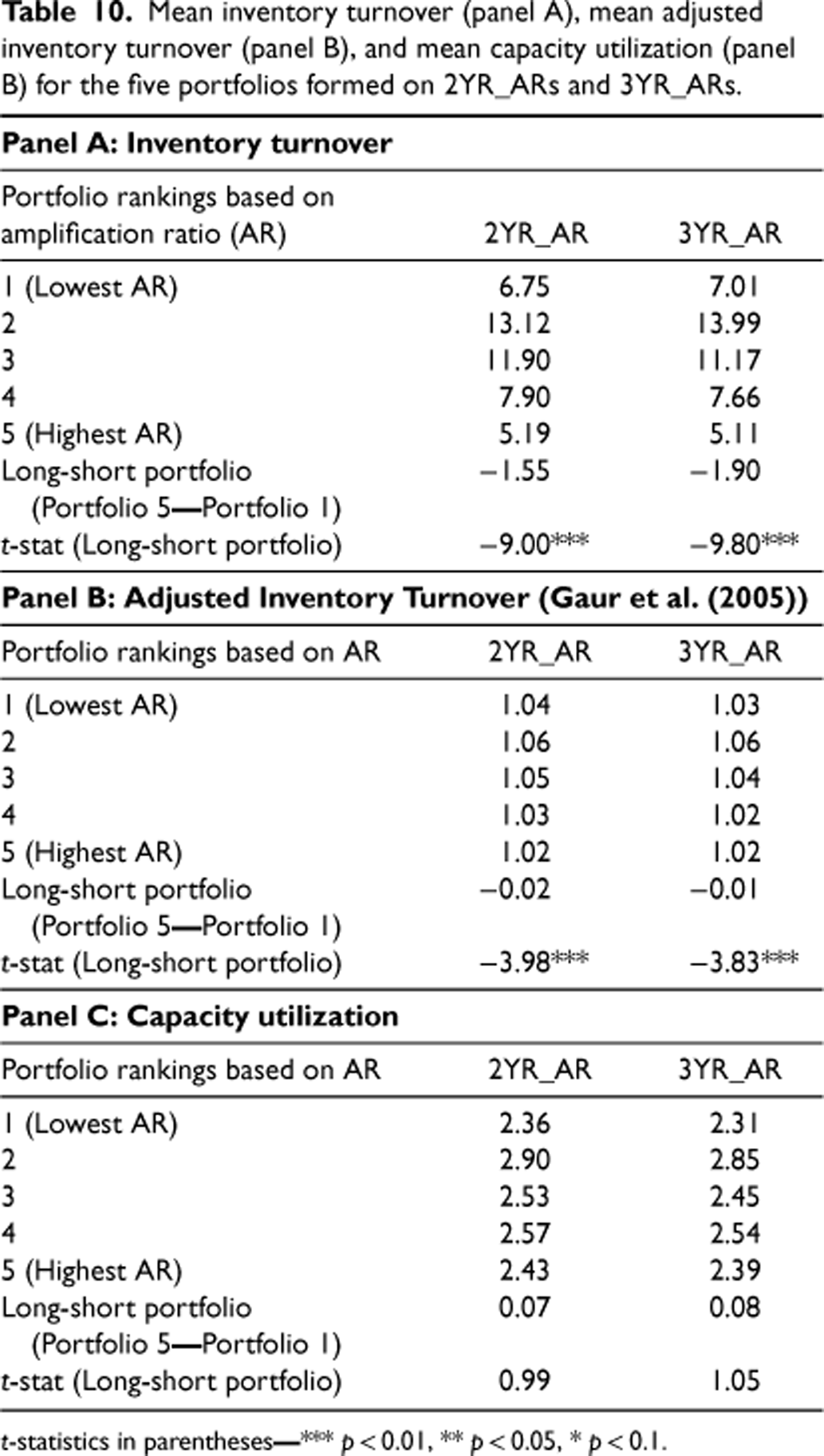
Mean inventory turnover (panel A), mean adjusted inventory turnover (panel B), and mean capacity utilization (panel B) for the five portfolios formed on 2YR_ARs and 3YR_ARs.
Mean inventory turnover (panel A), mean adjusted inventory turnover (panel B), and mean capacity utilization (panel B) for the five portfolios formed on 2YR_ARs and 3YR_ARs.
t-statistics in parentheses
Panel A reports the inventory turnover results. There is no evident trend in inventory turnover from the lowest AR portfolio (Portfolio 1) to the highest AR portfolio (Portfolio 5). For the portfolios based on 2YR_ARs, the mean inventory turnover of Portfolio 1 is 6.75. It then increases for Portfolios 2, and then decreases for Portfolios 3, 4, and 5. However, if we ignore Portfolio 1, there is a monotonic decreasing trend from Portfolios 2–5. The mean inventory turnover of Portfolio 5 is 5.19, significantly lower than 6.75, the mean inventory turnover of Portfolio 1. The results are similar when the portfolios are formed using the 3YR_ARs.
To explore the sensitivity of the relationship between the BWE and inventory turnover, we use the adjusted inventory turnover (AIT) metric developed by Gaur et al. (2005). AIT adjusts the inventory turnover for factors that explain the normal variation in the inventory turnover of firms. The details of estimating AIT are in the E-companion. Higher values of AIT indicate better inventory performance. Panel B reports the AIT results. There is no evident trend in AIT from Portfolio 1 to 5. However, if we ignore Portfolio 1, there is a monotonic decreasing trend from Portfolios 2 to 5. The mean AIT of Portfolio 5 is significantly lower than the mean AIT of Portfolio 1. We also estimated the abnormal excess inventory using the approach in Wu and Lai (2022), and the conclusions are very similar to the results in Panels A and B. The details of this analysis are in the E-companion.
The results of Panels A and B suggest a nonmonotone relationship between the BWE and inventory turnover, but this relation is not conclusive with only five portfolios. To explore this further, we implemented the moving portfolio analysis as in Chen et al. (2007) (see the E-companion for details). The analysis shows that the behavior of inventory turnover is nonmonotonic. It depicts an increasing-decreasing behavior as we move from low ARs to high ARs portfolios, which is consistent with the results using the five portfolios in Panels A and B. Overall, the results do provide some evidence to suggest that the BWE has a negative impact on inventory turnover.
Given that ARs have an increasing-decreasing effect on inventory turns, we examine the relationship between ARs and stock returns when it has a negative impact on inventory turns. From the moving portfolio analysis, we inferred that ARs has a negative impact on inventory in nearly 60% of the sample. We divide these firms into five quintiles based on ARs, where firms in the lowest (highest) quintile of ARs comprise Portfolio 1 (Portfolio 5). The E-companion reports the mean monthly returns of the five portfolios formed using 2YR_ARs and 3YR_ARs. Focusing on the returns for the portfolios formed using the 2YR_ARs, the long-short portfolio that buys Portfolio 5 and sells Portfolio 1 yields returns of 0.11% per month, statistically indistinguishable from zero. The results are similar when the portfolios are formed using the 3YR_ARs.
Panel C reports the capacity utilization results. There is no evident trend in capacity utilization from the lowest AR portfolio (Portfolio 1) to the highest AR portfolio (Portfolio 5). For the portfolios based on 2YR_ARs (3YR_ARs), the mean capacity utilization for Portfolio 5 is 2.43 (2.39), higher than 2.36 (2.31) the mean capacity utilization for Portfolio 1. However, the difference is statistically indistinguishable from zero.
As a sensitivity analysis, we repeated the analysis of Table 10 using standardized Z scores for inventory turnover and capacity utilization (see the E-companion). The conclusions from the standardized and unstandardized inventory turnover results are similar. The conclusions regarding trends across the five portfolios from the standardized and unstandardized capacity utilization are similar. However, when capacity utilization is standardized, the difference between Portfolios 5 and 1 is significant, but it is not significant when capacity utilization is unstandardized.
We next examine the link between the BWE and accounting-based profitability measures using the following four measures (Baron et al., 2023; Gaur et al., 2005; Mackelprang and Malhotra, 2015):
Net return on assets (NROA): Net income before extraordinary items normalized by the average of the start of the year and end of the year total assets. Net margin (NM): Net income before extraordinary items normalized by net sales. Gross return on assets (GROA): Gross income normalized by the average of start of the year and end of the year total assets. Gross margin (GM): Gross income normalized by net sales. Leverage: Sum of short-term and long-term debt scaled by total assets in year t Log of Total Assets: Natural log of total assets in year t Sales Growth: (Sales in year t—sales in year t − 1)/sales in year t − 1 Book-to-Market: Book value of shareholders’ equity in year t/market value of equity in year t
We follow the regression approach of Baron et al. (2023) in our analysis. We use the following four control variables from Baron et al. (2023) that have been shown in the literature to affect profitability:
Baron et al. (2023) also used demand persistency and sales volatility in their analysis, which are not included in our analysis as these variables were consistently insignificant in Baron et al. (2023). ARs are measured in October–December of calendar year t. All control variables are measured at the end of the fiscal year t that ends on or after December 31 of the calendar year t. All variables are winsorized at the 5% level in each tail. The results are estimated using panel regressions with firm and year-fixed efforts. The t-statistics are computed using robust standard errors.
Table 11 presents the regression results based on 2YR_ARs and 3YR_ARs. Models 1 to 4 are based on normalizing net income or gross income by total assets. Focusing on the 2YR_ARs, the relationships between AR and NROA are statistically insignificant. The results are similar when GROA is the dependent variable or when 3YR_ARs are the independent variable.
Analysis of the relationship between ARs and accounting-based profitability measures.
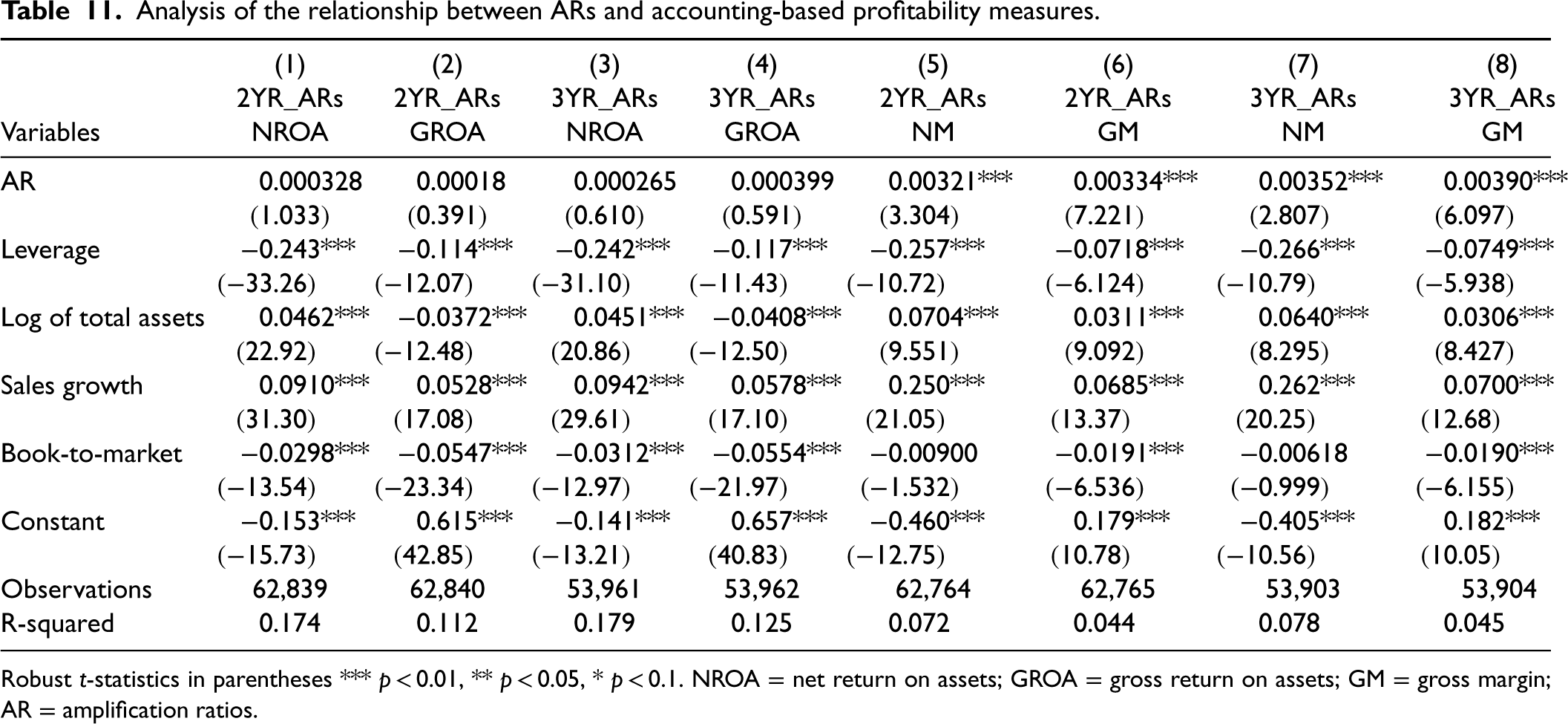
Robust t-statistics in parentheses *** p < 0.01, ** p < 0.05, * p < 0.1. NROA = net return on assets; GROA = gross return on assets; GM = gross margin; AR = amplification ratios.
Models 5 to 8 are based on normalizing net income or gross income by sales. Focusing on the 2YR_ARs, the relationships between AR and NM are positive and statistically significant, contrary to expectations. The results are similar when GM is the dependent variable or when 3YR_ARs are the independent variable. However, these significant relationships do not seem to be economically significant. For example, an increase in AR by one unit, increases NM and GM by only about 0.3%. Furthermore, adding AR as an independent variable has very little impact on r-squares. In untabulated results, we replace the values of ARs with decile-based ranks of ARs. The conclusions are very similar to the results in Table 11. Overall, it seems that ARs do not have any significant impact on ROAs measures. Although ARs have a positive impact on margin measures, the positive impact on margin does not seem to be economically significant.
We use the results of our analysis on the relationships between ARs and OPMs and ARs and profitability to explain the insignificant relationship between the BWE and stock returns. We have argued that the link between the BWE and stock returns is through OPMs. As discussed in Section 2, the literature collectively mentions several OPMs that can be negatively impacted by the BWE. However, data to empirically test the relationship between the BWE and several of these OPMs is not available. Since inventory data is widely available, researchers have focused on the relationship between the BWE and inventory. Although we find that the lowest AR firms (Portfolio 1) have better inventory performance than the highest AR firms (Portfolio 5), the relationship is not monotonic as we move from Portfolio 1 to portfolio 5. Baron et al. (2023) and Mackelprang and Malhotra (2015) also find that BWE and inventory performance are negatively correlated. Using data from a supermarket chain, Yao et al. (2021) find that higher BWE is associated with higher inventory. Overall, there is evidence that the BWE has a negative impact on inventory performance, consistent with expectations. We also analyzed the impact of ARs on capacity utilization but found no evidence of any impact.
A natural extension of the theory of the negative impact of the BWE on OPMs is that this will have a negative impact on profitability. We test this using accounting-based measure of ROAs and margins. The relationships between ARs and ROAs measures are statistically insignificant. The relationships between ARs and margin measures are positive and significant. However, these significant relationships do not seem to be economically significant. These results are consistent with the results of Baron et al. (2023), who note that their findings suggest that the BWE has little, if any, impact on profitability. Mackelprang and Malhotra (2015) find that the linear (quadratic) relationship between their measure of the BWE and ROA is significantly negative (positive), but the relationship between the BWE and operating margin is insignificant. Overall, the BWE does not seem to have an economically significant impact on profitability. This could explain our finding of statistically insignificant relationship between the BWE and stock returns.
Conclusions and Discussions
This paper examines the relationship between the BWE and stock price performance. The empirical analysis is based on data from 1985 to 2018 from about 7,200 publicly traded firms and about 64,000 firm-years. Consistent with Baron et al. (2023), we find that most results are statistically indistinguishable from zero. The few marginally significant results that we find suggest a positive relationship between the BWE and stock returns rather than the expected negative relationship. Besides, these marginally significant results do not hold when alternate methods are used to test the relationships - either the sign of the relationship changes or the results lose their significance. These conclusions are robust when we segment the sample by size, industry, and time periods. We also do not find a significant relationship between the BWE and stock returns for samples based on the propagation of the BWE from customers to suppliers. We do find some evidence to suggest that the BWE has a negative impact on inventory turnover. However, we do not find similar evidence for capacity utilization. The relationships between the BWE and ROAs measures are statistically insignificant. For margin measures, the relationships are positive and statistically significant but not economically significant.
Our results have several implications. The common belief is that the BWE can have a significant negative impact on financial performance, and both practitioners and academicians advocate for dampening the BWE. We find that the BWE has little impact on financial performance. Given this, firms considering dampening the BWE must be careful as dampening strategies may require investment and resources that may outweigh the benefits. Further, organizational and incentive issues may prevent firms from implementing strategies that could dampen the BWE.
Different firms in the same industry face some operating factors that are similar and others that are different. The analytical literature attributes the BWE to rational responses by the firm to its operating factors. If this is the case, then it may be optimal for some firms to not bullwhip and others to bullwhip. Most of the firms that do not bullwhip are smoothing production, which has its own costs. Our results suggest that there is no difference in the performance of firms that do not bullwhip and firms that bullwhip. An implication of our result is that firms might be optimally choosing their bullwhip levels based on their own operating factors. Given this, moving away from the current level of the BWE may not be economically beneficial.
The results of our paper are surprising and puzzling. However, we hope that our paper and the other papers addressing this issue can prompt conversations among researchers and practitioners on why firms continue to bullwhip despite the theoretical prediction that the BWE has a significant negative impact on financial performance. This could provide more guidance to firms on dealing with the BWE.
We have some suggestions for future research. First, the original description of the BWE in Lee et al. (1997a) and much of the subsequent analytical work on the BWE is based on the information flow measure where the BWE is measured based on the variances of order flows. While it would be ideal in empirical work to also measure the BWE using the information flow measure, information on order flows is not publicly available. Given the data availability constraints, much of the empirical research on the BWE based on publicly traded firms uses the material flow measure, which compares the variance of order receipts with the variance of sales. Our analysis is also based on the material flow measure. Future research could examine if BWE can be measured in better ways. Furthermore, data from publicly traded firms are aggregated on a quarterly basis. Future research could also explore whether different levels of time aggregation affect the relationship between the BWE and stock returns.
Second, there could be omitted variables related to unobservable firm characteristics, for example, managerial expertise and experience, and environment variables etc., that may be correlated to both the BWE and financial performance. While such omitted variables could bias the relationship between AR and financial performance, it is not necessary that these biases would be such that the relationship between AR and financial performance is insignificant. Future research could explore the omitted variable bias to provide a more comprehensive analysis of the relationship between the BWE and financial performance.
Third, given the importance of the BWE, we need more balance between analytical, experimental, and empirical research. Research on the BWE has been dominated by analytical and experimental work. While this has contributed to our understanding of the BWE, it needs to be complemented by empirical research. Although empirical research can be based on field studies or proprietary data sets, more empirical research is needed that is based on large samples using objective and widely available data. Empirical research is needed to validate the hypotheses, implications, and prescriptions from analytical and experimental research on the BWE.
Finally, we need more balance on the BWE issues that are being researched. It is clear from the literature that much of the research on the BWE is focused on documenting the existence of the BWE, identifying the factors that cause it, and developing strategies to mitigate it. Much of this research is based on the belief that the BWE has a negative impact on financial performance. Whether this is the case or not is an empirical issue, and more research is needed on this issue.
Supplemental Material
sj-pdf-1-pao-10.1177_10591478231224936 - Supplemental material for The Bullwhip Effect and Stock Returns
Supplemental material, sj-pdf-1-pao-10.1177_10591478231224936 for The Bullwhip Effect and Stock Returns by Vinod Singhal and Jing Wu in Production and Operations Management
Footnotes
Acknowledgments
The authors thank Subodha Kumar (the department editor), the associate editor, and two referees, whose constructive comments have significantly improved the paper. We also thank Jefferey Callen (University of Toronto), Brian Jacobs (Pepperdine University), and Manpreet Hora (Georgia Institute of Technology) for their feedback on the paper.
Declaration of Conflicting Interests
The authors declared no potential conflicts of interest with respect to the research, authorship, and/or publication of this article.
Funding
The authors received no financial support for the research, authorship, and/or publication of this article.
How to cite this article
Singhal V and Wu J (2024) The Bullwhip Effect and Stock Returns. Production and Operations Management 33(1): 303–322.
References
Supplementary Material
Please find the following supplemental material available below.
For Open Access articles published under a Creative Commons License, all supplemental material carries the same license as the article it is associated with.
For non-Open Access articles published, all supplemental material carries a non-exclusive license, and permission requests for re-use of supplemental material or any part of supplemental material shall be sent directly to the copyright owner as specified in the copyright notice associated with the article.