Should an Incumbent Store Deter Entry of a Socially Responsible Retailer?

Abstract

Should an incumbent for-profit retailer deter a “socially responsible” store from entering the market? As a differentiation strategy to avoid direct price competition with well-established retailers, some socially responsible stores (or brands) enter the market with a “pre-commitment” to donate a certain proportion of their (A) profits or (B) revenues to charities. Because these charitable donations generate a “warm-glow” effect for consumers, these socially responsible stores can use pre-committed donations to gain market access. In this paper, we present a game-theoretic model in which a socially responsible retailer enters the market to compete with an incumbent for-profit retailer. We determine and compare the incumbent retailer’s deterrence strategies (i.e., deter or tolerate) across different types of socially responsible stores. Our equilibrium analysis generates the following insights. First, the incumbent retailer’s deterrence strategy depends on its cost advantage over the socially responsible store, and hinges upon the socially responsible store’s entry cost, pre-commitment level, and its warm-glow effect. Second, even if the incumbent retailer can profitably deter the socially responsible retailer’s entry, the incumbent retailer can actually be better off by tolerating instead of deterring its entry when the socially responsible store’s entry cost is low and the incumbent store’s cost advantage is not significant. Third, relatively speaking, a type (B) store that donates a portion of its revenue is more vulnerable unless it can generate a much higher warm-glow effect. We extend our analysis numerically to examine the case when the pre-committed proportion is endogenously determined and obtain similar structural results.

1. Introduction

New generations are more socially conscious: 73% of Americans consider companies’ social causes when making purchasing decisions (Mintel, 2018). Because social causes generate the “warm-glow” effect for socially conscious consumers, a socially responsible store (hereafter, social retailer) can use “pre-committed” charitable donations (besides lower selling prices to gain market access) to create a new threat for the incumbent for-profit retailer (hereafter, for-profit retailer).

Social retailers can pre-commit to donating a certain proportion of their (A) profits or (B) revenues to charities (see Chen, 2021 for a list of 35 such retailers). ¹ Two examples of type (A) social retailers are Toms and Ivory Ella. ² Toms donates one-third of its profits for grassroots good, including cash grants and partnerships with community organizations, to drive sustainable change, whereas Ivory Ella donates 10% of its profits toward saving elephants. Two examples of type (B) social retailers are Cotopaxi and Judy. ³ Cotopaxi donates 1% of its yearly revenue to nonprofits making sustainable changes in poverty alleviation, while Judy donates 1% of its annual revenue to the Los Angeles Fire Department Foundation, which provides essential equipment and training to supplement city resources. These charitable donations generate the “warm-glow” effect for consumers who shop at social retailers (cf. Andreoni, 1990; Harbaugh, 1998).

While consumers welcome social retailers to enter the market and thrive, this movement can also trigger incumbent for-profit retailers to proactively reduce their prices to “deter” the entry of social retailers. Therefore, our intent is to examine and compare the incumbent store’s deterrence strategies between type (A) and type (B) stores. We choose to compare these two types of socially responsible stores by design because they are commonly seen. More importantly, because of their similarity (i.e., donation based on profit versus revenue), their warm-glow effects are analytically comparable so that we can compare the deterrence strategies of the incumbent store across different types by focusing on one variation. ⁴ In particular, we aim to answer the following research questions:

What is the entry and pricing strategy of a social retailer in the presence of an incumbent for-profit retailer?

Should the incumbent retailer deter or tolerate the entry of the social retailer?

How does the incumbent retailer’s deterrence strategy differ between different types of social retailers?

In this paper, we present a two-stage Stackelberg model of a social retailer who enters a market to compete with an incumbent for-profit retailer. The social retailer incurs an entry cost and pre-commits to donate a certain proportion of its profit (if type (A)) or revenue (if type (B)). Consumers in the market are heterogeneous in their utility from shopping at both retailers and they obtain a warm-glow effect from shopping at the social retailer.

To answer our first research question, we first analyze the strategic interactions among utility-maximizing consumers, a profit-maximizing retailer, and a type (A) social retailer. We find that a type (A) social retailer’s optimal price depends on the incumbent retailer’s price, and its profit and its entry condition depend on its cost of entry. Next, regarding our second research question, we discover that the deterrence strategy employed by the incumbent retailer depends on its unit-cost advantage over the social retailer, as well as the social retailer’s entry cost. Interestingly, even if the incumbent retailer can profitably deter the social retailer’s entry, the incumbent retailer can be better off by tolerating this entry unless it has a substantial competitive advantage over the social retailer (due to the incumbent’s significantly lower unit cost or the social retailer’s high entry cost).

We also examine the entry of a type (B) social retailer. We find that the aforementioned results associated with our first and second research questions remain valid in the case of a type (B) store. Additionally, we derive additional insights concerning a social retailer of type (B). Specifically, the donation proportion plays a more important role in the pricing decisions of a type (B) retailer. Specifically, to cover the donations, a type (B) social retailer needs to charge a higher price and obtain a smaller market share. Due to this challenge, ceteris paribus, a type (B) social retailer’s entry poses a smaller threat to the incumbent retailer. For this reason, one may expect that the incumbent retailer is more tolerant toward a type (B) social retailer. Interestingly, we find an opposite result: the incumbent store is actually more likely to deter the entry of a type (B) social retailer that commits to donate a certain proportion of its revenue.

Regarding the third question, we analytically demonstrate that even if the two stores generate the same level of warm-glow effect, the incumbent store R may adopt different deterrence strategies against them. Specifically, we find that the incumbent is more aggressive in deterring a type (B) store (that donates a proportion of its revenue) than a type (A) store (that donates a proportion of its profit), unless a type (B) store can generate a significantly higher warm-glow effect. Our results are informative for policymakers and entrepreneurs aiming to establish social retailers as they show how an incumbent retailer reacts to entry threats made by different types of social retailers.

By extending our analysis to the case when the pre-committed proportion is “endogenously determined” by each type of social retailer. Through our extensive numerical analysis, we find the same structural results continue to hold: even when both social retailers set the pre-committed proportion optimally, the incumbent store is more likely to tolerate the entrance of a type (A) store than a type (B) store. Also, we examine how the social store’s entry cost and the incumbent store’s cost advantage affect the optimal proportion, and the corresponding equilibrium outcomes (such as the social store’s selling price, and the profit of the social store and the incumbent store). We find that these quantities behave in an intuitive manner in most instances. However, one may conjecture that a type (B) store, which donates a portion of its revenue, would always donate more than a type (A) store that donates a portion of its profit. Interestingly, this conjecture is not necessarily true: we find that it is also possible for a type (A) store to donate a larger amount than a type (B) store when the proportion is “endogenously determined”.

This paper is organized as follows. We review the relevant literature in Section 2. After we define our model preliminaries in Section 3, we analyze the potential entry of a type (A) store and its impact in Section 4. We analyze the implications of the potential entry of a type (B) store in Section 5. We then compare the two types of stores in Section 6. In Section 7, we expand the analysis by considering endogenously determined donating proportion to show the robustness of our structural results. Finally, we conclude in Section 8.

2. Literature Review

Our study is related to studies on market entry, mixed oligopoly, and socially responsible retailers.

The market-entry literature establishes the notion of an incumbent’s decision to lower its price below the profit-maximizing price to “deter” the entry of a for-profit competitor. This literature mainly focuses on how a for-profit firm can deter the entry of a for-profit competitor of the same type and suggests deterrence tools such as pricing (Bain, 1949), strategic commitment (Spence, 1977, 1979), long-term contracts (Aghion and Bolton, 1987), cost signaling (Srinivasan, 1991), bundle pricing (Nalebuff, 2004), or discount contracts (Ide et al., 2016). Overall, these papers focus on the deterrence tools or the market structure rather than focusing on the entrant characteristics. (We refer the reader to Hall (2008) for a review of the market-entry literature.) More recently, Gao et al. (2017) examine the entry of copycats and show that the incumbent firm can deter the copycat from entering by selling a higher-quality product. There are also some papers in the supply chain competition literature (e.g., Corbett and Karmarkar, 2001; Korpeoglu et al., 2020) that analyze the market entry and competition of identical for-profit firms. Our work contributes to the market-entry literature on several fronts. First, unlike the literature that studies the entry of for-profit retailers, we examine the entry of a social retailer that pre-commits to donating a certain proportion of its profit (type A) or revenue (type B). This social commitment adds a new dimension to price competition because it also creates a warm-glow effect for the social retailer’s customers. Our work also compares the entry of the two types of social retailers.

Our work is also related to mixed oligopoly in which firms compete with different objectives (De Fraja and Delbono, 1990). (We refer the reader to Zhou et al. (2023) for a review of the recent literature). Our model differs from the literature on several fronts. First, our work considers the market entry of a social retailer that maximizes its profit but is subject to donating a certain proportion of its profit or revenue. Indeed, a major contribution of our paper is to compare the entry of these two types of social retailers. Second, we consider the warm-glow effect that consumers receive from shopping at the social retailer.

Our work also contributes to the literature on socially responsible retailers. ⁵ There is a body of work that recognizes the “warm glow” that consumers receive from shopping at socially responsible retailers (e.g., Bloom et al., 2006; Strahilevitz, 1999). Some more recent papers study the impact of this warm glow on operational decisions. Arya and Mittendorf (2015) investigate the impact of a government subsidy in an environment with one supplier and one socially responsible retailer that commits to donating a certain number of goods. Gao (2020) studies the pricing decisions of a firm that commits to donating a proportion of its revenue to charity without considering any competition. Our work contributes to this literature by incorporating the warm-glow effect in a new context so that we can explore the entry strategy of a socially responsible retailer and the deterrence strategy of an incumbent retailer.

3. Model Preliminaries

We consider a Stackelberg competition model that involves an incumbent for-profit retailer (store R) and an entrant social retailer (store S). For a consumer who shops at the incumbent store R, we assume that the consumer utility satisfies:

$$U_r=v-p_r,$$

(1)

where $v\sim U[0,1]$ captures the heterogenous consumer valuation for a certain product, and $p_r(<1)$ is the selling price set by store R.

For store R and store S, let $c_r$ and $c_s$ be their unit costs, respectively. (Throughout this paper, subscripts $r$ and $s$ are used to denote stores R and S, respectively.) Because store R has sourced from its suppliers with a proven sales record over an extended period of time, we assume that store R has a “cost advantage” over store S so that the parameter $\alpha \equiv c_r/c_s<1$ . ⁶ Due to store S’s cost disadvantage (as $c_s>c_r$ ), store S (the new entrant) has to differentiate itself from the incumbent by creating the warm-glow effect so that consumers can obtain a higher valuation when shopping at store S. To create the warm-glow effect, we focus on the case when store S is committed to differentiate itself from store R by donating a proportion $\gamma \in (0,1)$ of its profit to charities as a type (A) store, or by donating a proportion $\gamma \in (0,1)$ of its revenue to charities as a type (B) store. ⁷ Here, $\gamma$ corresponds to a “generic” donating proportion of profit/revenue for a type (A)/(B) store.

To obtain tractable analytical results, we first treat $\gamma \in (0,1)$ as an exogenously given parameter in our base model. In doing so, we establish structural results that serve as “benchmarks” for further examination. For instance, different types of store S would commit to donating different proportions (i.e., ${\gamma }^A\ne {\gamma }^B$ ) especially when ${\gamma }^j,j=A,B,$ is determined endogenously by each type $j$ store. This observation motivates us to consider $\gamma$ as an endogenous decision for each type of store S in Section 7. Specifically, in Section 7, we conduct a comprehensive numerical study for the case when $\gamma$ is endogenously determined, and we find that our structural (benchmark) results of the base model continue to hold. For any exogenously given $\gamma >0$ in our base model, we assume that the consumer utility for shopping at store S takes the following form:

$$U_s^j={\beta }^j(\gamma )\cdot v-p_s,j\in \{A,B\},$$

(2)

where $p_s$ is the price set by store S. Here, the “warm-glow effect” is captured by a function ${\beta }^j(\gamma )\ge 1$ , where ${\beta }^j(\gamma )$ is an increasing function of $\gamma$ . For example, the warm-glow effect can take a linear form (i.e., ${\beta }^j(\gamma )=(1+b^j\cdot \gamma )$ with $b^j>0$ so that consumers have a higher valuation when shopping at a type (A)/(B) store S). Hence, by donating a proportion $\gamma \in (0,1)$ of its profit or revenue to charities, store S can leverage its higher consumer valuation ${\beta }^j(\gamma )\cdot v\equiv (1+b^j\cdot \gamma )v>v$ to compete against store R despite of its cost disadvantage $\alpha \equiv c_r/c_s<1$ .

If one considers (2) in isolation, then store S can be interpreted as the store that offers a vertically differentiated product that is better than store R. Therefore, our market-entry game is similar to those examined in the literature (e.g., Hall, 2008). However, if one considers (2) in conjunction with store S’s profit function, then a fundamental difference emerges. In a traditional market-entry game, one store makes a “separate” investment to develop a vertically differentiated product (e.g., invest in quality for a higher quality product). However, in our context, store S’s investment is the proportion $\gamma$ that is “embedded” in the profit (for type (A)) or in the revenue (for type (B)) to create the differentiation through the warm-glow effect ${\beta }^j(\gamma )$ . Consequently, the analysis and store R’s deterrence strategy is different from the traditional market-entry game considered in the literature (e.g., Gao et al., 2017; Corbett and Karmarkar, 2001; Korpeoglu et al., 2020).

Certainly, the exact function form of the warm-glow effect ${\beta }^j(\gamma )$ would depend on the type of charity and the consumer segment that store S will be focusing on. For example, a store S may be owned by a female who pre-commits to donate a proportion of its profit (or revenue) to the National Breast Cancer Foundation by selling a product targeting female consumers. As a generic model, we do not model a specific charity and a specific consumer segment in our analytical analysis; instead, we consider an implicit function form ${\beta }^j(\gamma )$ in the base model of exogenously given $\gamma$ so that our model can be applied to different charities. Later on in Section 7, we capture this issue succinctly by considering a general function form ${\beta }^j(\gamma )=1+b^j\cdot {\gamma }^t$ , where the parameters $b^j$ and $t>0$ ; and we conduct a comprehensive numerical study by varying the parameters $b^j$ and $t$ .

3.1. A Sequential Market-Entry Game: Should Store R Deter or Tolerate Store S’s Entry?

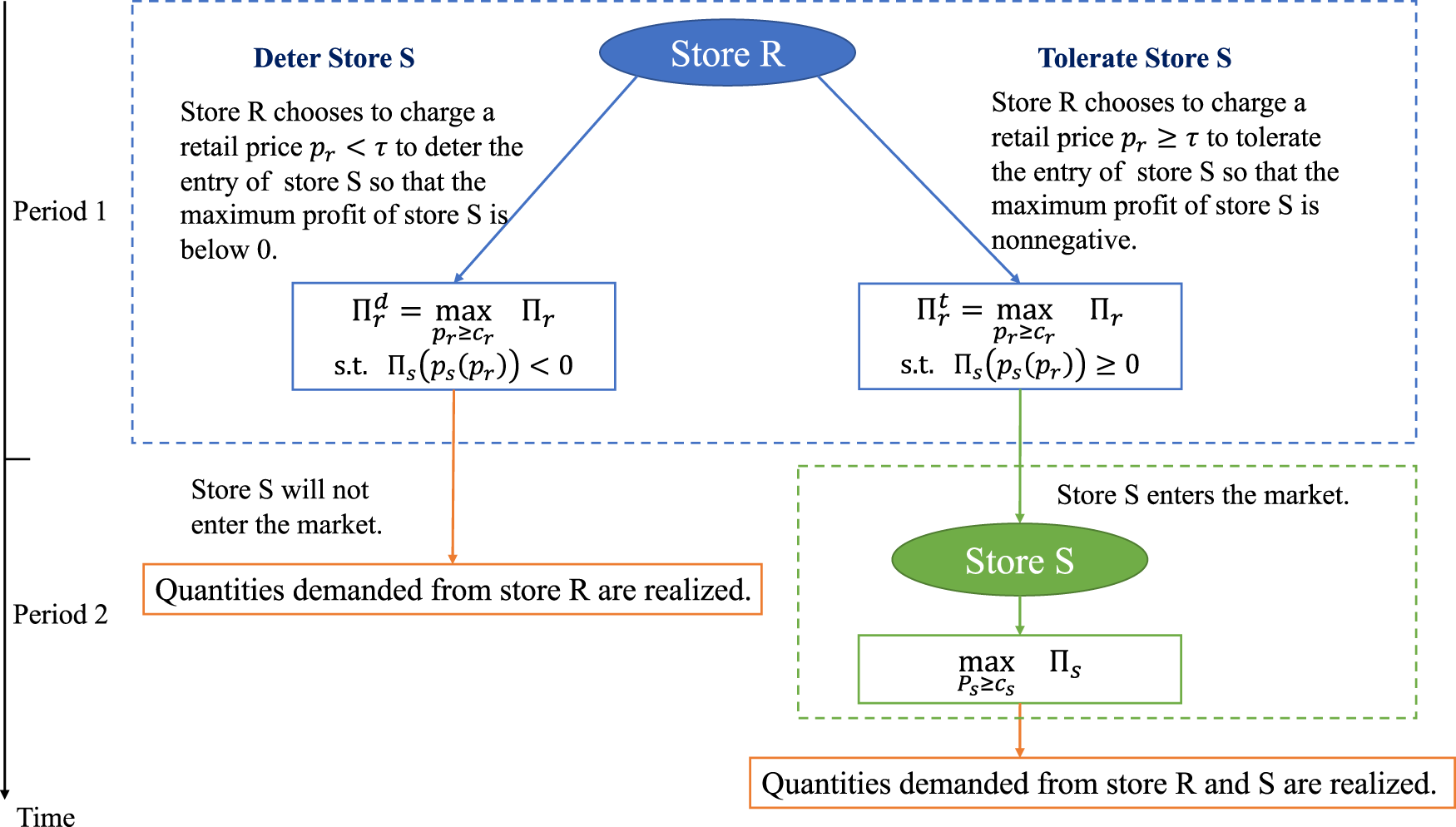
The dynamic decisions to be made by the incumbent store R and the new entrant store S can be modeled as a two-period sequential game as depicted in Figure 1.

Figure 1.

A market-entry game between the incumbent store R and a “generic” store S (of type (A) or (B)).

In period 1, store S has not yet entered and incumbent store R can choose its price $p_r$ to either deter or tolerate store S’s entry (the blue box in Figure 1). To deter, store R can set $p_r$ below a threshold $\tau$ (to be determined) so that store S cannot afford to enter. Consequently, store R operates as a monopoly with the set price $p_r$ in period 2 and the game ends. If store R chooses to tolerate by setting $p_r$ above the threshold $\tau$ , then store S can afford to enter in period 2 by incurring an entry cost $k$ . (This entry cost $k$ can represent the present value of loan repayments store S has to make using its future earnings to cover its initial investment.) Upon entry, store S observes $p_r$ and competes with store R in a duopoly in period 2 by choosing its own price $p_s$ that takes its unit cost $c_s$ into consideration (the green box in Figure 1). ⁸

3.2. Backward Induction Steps for Determining Equilibrium Strategies

We now describe how we solve the sequential game that involves the potential entry of a generic store S (of type $j$ , $j=A,B$ ) via backward induction. We shall use this approach to examine the potential entry of a type (A) and a type (B) store S in Sections 4 and 5, respectively. In preparation, let us first describe consumer demand. Then, we formulate store S’s problem in period 2 (the green box in Figure 1) and then store R’s problem in period 1 (the blue box in Figure 1).

3.2.1. Consumer Demand

Each retailer’s consumer demand depends on store R’s deterrence strategy. First, if store R chooses to deter any type of store S’s entry by setting $p_r<\tau$ , it operates as a monopoly so that only consumers with utility $U_r=v-p_r\ge 0$ will buy the product from store R. It follows from (1), the consumer demand $q_r$ for store R is:

$$q_r=1-p_r.$$

(3)

Next, if store R sets its price $p_r\ge \tau$ in period 1 to tolerate a type $j=A,B$ store S’s entry and store S sets its price $p_s^j$ in period 2, then a consumer will purchase from store R only when $U_r\ge 0$ and $U_r\ge U_s^j$ ; or purchase from store S only when $U_s^j\ge 0$ and $U_s^j\ge U_r$ . By considering $U_r$ and $U_s^j$ given in (1) and (2), the consumer demand $q_r^j$ for store R and $q_s^j$ for a type $j$ store S satisfy:

$$\begin{array}{rl}{q}_r^j& =\{\begin{array}{ll}0& \text{if}{p}_s\le {\beta }^j(\gamma )\cdot p_r,\\ \frac{p_s-p_r}{{\beta }^j(\gamma )-1}-p_r& \text{if}{\beta }^j(\gamma )\cdot p_r<p_s<{\beta }^j(\gamma )-1+p_r,\\ 1-p_r& \text{if}{p}_s\ge {\beta }^j(\gamma )-1+p_r,\end{array}\end{array}$$

(4)

$$\begin{array}{rl}{q}_s^j& =\{\begin{array}{ll}1-\frac{p_s}{{\beta }^j(\gamma )}& \text{if}{p}_s\le {\beta }^j(\gamma )\cdot p_r,\\ 1-\frac{p_s-p_r}{{\beta }^j(\gamma )-1}& \text{if}{\beta }^j(\gamma )\cdot p_r<p_s<{\beta }^j(\gamma )-1+p_r,\\ 0& \text{if}{p}_s\ge {\beta }^j(\gamma )-1+p_r.\end{array}.\end{array}$$

(5)

Because store S’s warm-glow effect ${\beta }^j(\gamma )$ depends on $\gamma$ , $q_r^j$ and $q_s^j$ also depend on $\gamma$ through ${\beta }^j(\gamma )$ .

3.2.2. Store S’s Problem in Period 2

Using the consumer demand functions as stated above, we now formulate store S’s problem in period 2 (the green box in Figure 1) in Section 3.2.2, followed by store R’s problem in period 1 (the blue box in Figure 1) in Section 3.2.3. To begin, if store R deters store S’s entry, then store S’s problem is moot. Hence, store S’s problem is only relevant when store R sets $p_r\ge \tau$ in period 1 to tolerate store S’s entry. In period 2, store S can set its best-response price $p_s$ to compete with store R in a duopoly upon observing $p_r$ set by store R in period 1. By considering its unit cost $c_s$ ( $\le \beta$ to eliminate trivial cases where store S can never make a profit) and the entry cost $k$ , store S can determine its best-response price $p_s$ that maximizes its net profit. For any given $p_r$ , store S can use the consumer demand $q_s$ given by (5) to formulate its problem as follows.

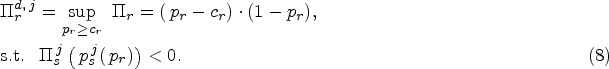
First, for a type (A) store S who commits to donate a proportion $\gamma$ of its profit, its problem in period 2 is to set its price $p_s^A(p_r)$ as the best response by solving:

$$\begin{array}{rl}& {\mathrm{\Pi }}_s^A(p_r)=\underset{p_s\ge c_s}{max}{\mathrm{\Pi }}_s=(1-\gamma )\cdot [(p_s-c_s)\cdot q_s^A-k],\\ & \text{s.t. }{q}_s^A=\{\begin{array}{ll}1-\frac{p_s}{{\beta }^A(\gamma )}& \text{if}{p}_s\le {\beta }^A(\gamma )\cdot p_r,\\ 1-\frac{p_s-p_r}{{\beta }^A(\gamma )-1}& \text{if}{\beta }^A(\gamma )\cdot p_r<p_s<{\beta }^A(\gamma )-1+p_r,\\ 0& \text{if}{p}_s\ge {\beta }^A(\gamma )-1+p_r,\end{array}\end{array}$$

(6)

where $q_s^A$ is given in (5). Hence, a type (A) store S will enter the market if and only if ${\mathrm{\Pi }}_s^A(p_r)\ge 0$ .

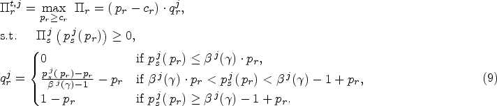
Similarly, for a type (B) store S who commits to donate a proportion $\gamma$ of its revenue to charities, its problem in period 2 is to choose its price $p_s^B(p_r)$ as the best response by solving:

$$\begin{array}{rl}{\mathrm{\Pi }}_s^B(p_r)& =\underset{p_s\ge c_s}{max}{\mathrm{\Pi }}_s=(1-\gamma )\cdot p_s\cdot q_s^B-(c_s\cdot q_s^B+k)\\ & =(1-\gamma )\cdot [(p_s-\frac{c_s}{1-\gamma })\cdot q_s^B-\frac{k}{1-\gamma }],\\ \text{s.t. }{q}_s^B& =\{\begin{array}{ll}1-\frac{p_s}{{\beta }^B(\gamma )}& \text{if}{p}_s\le {\beta }^B(\gamma )\cdot p_r,\\ 1-\frac{p_s-p_r}{{\beta }^B(\gamma )-1}& \text{if}{\beta }^B(\gamma )\cdot p_r<p_s<{\beta }^B(\gamma )-1+p_r,\\ 0& \text{if}{p}_s\ge {\beta }^B(\gamma )-1+p_r.\end{array}\end{array}$$

(7)

Hence, a type (B) store S will enter the market if and only if ${\mathrm{\Pi }}_s^B(p_r)\ge 0$ . From (7), we note that store S needs to charge $p_s\ge (c_s/(1-\gamma ))$ to ensure a positive gross margin and $p_s<{\beta }^B(\gamma )-1+p_r$ to ensure a positive demand. By noting that $p_r\le 1$ , we shall assume $c_s<(1-\gamma ){\beta }^B(\gamma )$ to rule out the trivial cases in which store S can never afford to enter the market.

By considering consumer utility given in (2) along with store S’s profit functions given in (6) and (7), it becomes clear that store S sacrifices a proportion $\gamma$ of its profit (or revenue) in exchange for the warm-glow effect as captured in (2). Also, because the proportion $\gamma$ generates the warm-glow effect ${\beta }^j(\gamma )$ , it creates a different dynamics than those traditional market-entry games considered in the literature as explained earlier. It is likely that different types of store S would commit to donating different proportions (i.e., ${\gamma }^A\ne {\gamma }^B$ ) as illustrated in the examples of Section 1, especially when these proportions are determined endogenously as examined in Section 7.

3.2.3. Store R’s Problem in Period 1

In period 1, store R can anticipate a type j store S’s best-response entry decision and price $p_s^j(p_r)$ (i.e., the optimal solution to problem (6) for $j=A$ and problem (7) for $j=B$ ). Then, we can formulate store R’s “deterrence strategy” problem (highlighted in the blue box of Figure 1) according to store R’s decision to deter or tolerate a type j store S’s entry.

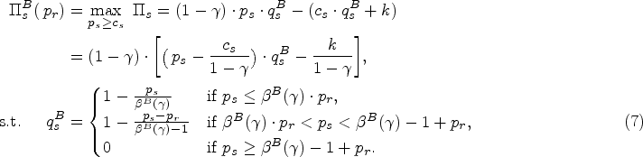
If store R chooses to deter a type $j$ store S’s entry by choosing $p_r$ to ensure ${\mathrm{\Pi }}_s^j(p_s^j(p_r))<0$ , then store R can operate as a monopoly. Hence, by considering store R’s monopoly demand $q_r$ given in (3), store R can determine its optimal price $p_r^{d,j}$ by solving:

$$\begin{array}{rl}& {\mathrm{\Pi }}_r^{d,j}=\underset{p_r\ge c_r}{sup}{\mathrm{\Pi }}_r=(p_r-c_r)\cdot (1-p_r),\\ & \text{s.t. }{\mathrm{\Pi }}_s^j(p_s^j(p_r))<0.\end{array}$$

(8)

Similarly, if store R tolerates store S’s entry by choosing $p_r$ to ensure ${\mathrm{\Pi }}_s^j(p_s^j(p_r))\ge 0$ , then by considering store R’s demand $q_r^j$ given in (4), store R determines its optimal price $p_r^{t,j}$ by solving:

$$\begin{array}{rl}& {\mathrm{\Pi }}_r^{t,j}=\underset{p_r\ge c_r}{max}{\mathrm{\Pi }}_r=(p_r-c_r)\cdot q_r^j,\\ & \text{s.t. }{\mathrm{\Pi }}_s^j(p_s^j(p_r))\ge 0,\\ & q_r^j=\{\begin{array}{ll}0& \text{if}{p}_s^j(p_r)\le {\beta }^j(\gamma )\cdot p_r,\\ \frac{p_s^j(p_r)-p_r}{{\beta }^j(\gamma )-1}-p_r& \text{if}{\beta }^j(\gamma )\cdot p_r<p_s^j(p_r)<{\beta }^j(\gamma )-1+p_r,\\ 1-p_r& \text{if}{p}_s^j(p_r)\ge {\beta }^j(\gamma )-1+p_r.\end{array}\end{array}$$

(9)

Here, superscripts $d$ and $t$ denote store R’s deterrence and tolerance strategies, respectively. Observe from (8) and (9) that store R’s problems depend on the store type $j$ and its warm-glow effect ${\beta }^j(\gamma )$ .

3.2.4. Store R’s Deterrence Strategy

By solving store R’s problems (8) and (9), we can determine store R’s deterrence strategy against a type $j$ store S as follows. First, by comparing store R’s optimal profit ${\mathrm{\Pi }}_r^{d,j}$ when deterring store S as given in (8) and ${\mathrm{\Pi }}_r^{t,j}$ when tolerating store S as given in (9), it is optimal for store R to deter the entry of a type $j$ store S if ${\mathrm{\Pi }}_r^{d,j}>{\mathrm{\Pi }}_r^{t,j}$ , and tolerate a type $j$ store S’s entry; otherwise. Meanwhile, store R chooses its equilibrium price $p_r^j$ that maximizes its profit (i.e., ${\mathrm{\Pi }}_r^j=max\{{\mathrm{\Pi }}_r^{d,j},{\mathrm{\Pi }}_r^{t,j}\}$ ). Second, we characterize a type $j$ store S’s equilibrium entry and pricing decisions in period 2. Specifically, if store R chooses to tolerate a type $j$ store S’s entry, we can retrieve a type $j$ store S’s corresponding equilibrium price $p_s^j(p_r^j)$ through substitution (otherwise, store S cannot enter).

In this section, we have described the process by which we solve the market-entry game between store R and a generic type of store S as depicted in Figure 1. We now proceed to delve into our analysis for each type of store S as follows. In Section 4, we analyze the case of a type (A) store S. Then, in Section 5, we analyze the case of a type (B) store S, followed by a comparison of our results associated with these two types of store S in Section 6.

4. Market-Entry Game between a Type (A) Store S and an Incumbent Store R

We now analyze the market-entry game between an incumbent store R and a potential entry of a type (A) store S. To do so, we solve a type (A) store S’s problem (6) in period 2 for any given store R’s price $p_r$ in Section 4.1. Then, in Section 4.2, we solve store R’s problems in period 1 as described in Section 3.2.3, followed by store R’s deterrence strategy as explained in Section 3.2.4.

4.1. Type (A) Store S’s Best-Response Pricing Strategy in Period 2

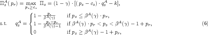
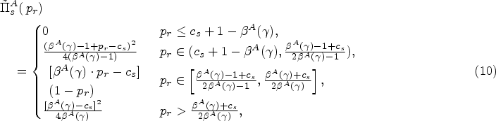
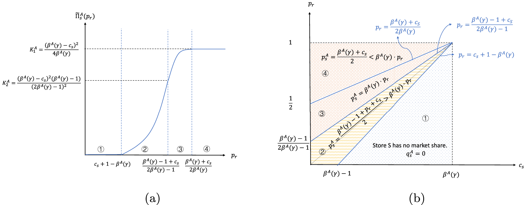
For any store R’s retail price $p_r$ (set in period 1), a type (A) store S solves problem (6) in period 2 as described in Section 3.2.2 by determining the optimal solution $p_s^A$ that represents the best-response price for a type (A) store S. From (6), we can rewrite the effective maximum profit ${\mathrm{\Pi }}_s^A(p_r)=(1-\gamma )\cdot ({\tilde{\mathrm{\Pi }}}_s^A(p_r)-k)$ , where ${\tilde{\mathrm{\Pi }}}_s^A(p_r)\equiv (p_s^A-c_s)\cdot q_s^A$ represents the maximum gross profit of store S without considering the donation proportion $\gamma$ or the entry cost $k$ . By solving (6), we get:

Lemma 1

Given any store R’s price $p_r$ , a type (A) store S’s maximum gross profit ${\tilde{\mathrm{\Pi }}}_s^A(p_r)$ satisfies:

$$\begin{array}{rl}& {\tilde{\mathrm{\Pi }}}_s^A(p_r)\\ & =\{\begin{array}{ll}0& p_r\le c_s+1-{\beta }^A(\gamma ),\\ \frac{({\beta }^A(\gamma )-1+p_r-c_s{)}^2}{4({\beta }^A(\gamma )-1)}& p_r\in (c_s+1-{\beta }^A(\gamma ),\frac{{\beta }^A(\gamma )-1+c_s}{2{\beta }^A(\gamma )-1}),\\ \begin{array}{l}[{\beta }^A(\gamma )\cdot p_r-c_s]\\ (1-p_r)\end{array}& p_r\in [\frac{{\beta }^A(\gamma )-1+c_s}{2{\beta }^A(\gamma )-1},\frac{{\beta }^A(\gamma )+c_s}{2{\beta }^A(\gamma )}],\\ \frac{[{\beta }^A(\gamma )-c_s{]}^2}{4{\beta }^A(\gamma )}& p_r>\frac{{\beta }^A(\gamma )+c_s}{2{\beta }^A(\gamma )},\end{array}\end{array}$$

(10)

and ${\tilde{\mathrm{\Pi }}}_s^A(p_r)$ is non-decreasing in $p_r$ .

Figure 2(a) illustrates store S’s maximum gross profit ${\tilde{\mathrm{\Pi }}}_s^A(p_r)$ for those four cases stated in (10). Because store S’s entry condition is ${\tilde{\mathrm{\Pi }}}_s^A(p_r)\ge k$ (so that store S’s net profit ${\mathrm{\Pi }}_s^A(p_r)=(1-\gamma )\cdot [{\tilde{\mathrm{\Pi }}}_s^A(p_r)-k]\ge 0$ ) and because ${\tilde{\mathrm{\Pi }}}_s^A(p_r)$ is nondecreasing in store R’s price $p_r$ , this entry condition holds only when store R sets its price $p_r$ sufficiently high. This explicit entry condition for store S will be used in Section 4.2 for determining store R’s deterrence strategy along with those thresholds $K_1^A$ and $K_2^A$ as explained later.

Figure 2.

Type (A) store S’s best-response pricing strategy: (a) store S’s gross profit ${\tilde{\mathrm{\Pi }}}_s^A(p_r)$ and (b) store S’s best-response price $p_s^A$ .

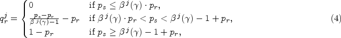
Next, observe from Lemma 1 that store S’s entry condition is violated if store R sets its price $p_r$ sufficiently low so that $p_r\le c_s+1-{\beta }^A(\gamma )$ . By ruling out this trivial case, we can determine the best-response price $p_s^A$ that depends on store R’s price $p_r$ , the warm-glow effect ${\beta }^A(\gamma )$ along with the proportion $\gamma$ as stated in the following proposition. Also, we can use the optimal price $p_s^A$ associated with the remaining three cases to retrieve the corresponding optimal quantity $q_s^A$ and the optimal profit ${\mathrm{\Pi }}_s^A(p_r)$ from (6) as follows.

Proposition 1

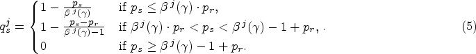
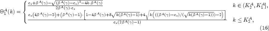
Suppose store R sets its price at $p_r$ so that $p_r>c_s+1-{\beta }^A(\gamma )$ and store S’s entry condition holds (i.e., $k\le {\tilde{\mathrm{\Pi }}}_s^A(p_r)$ , where ${\tilde{\mathrm{\Pi }}}_s^A(p_r)$ is given in Lemma 1). Then a type (A) store S’s best-response price $p_s^A$ , consumer demand $q_s^A$ , and retained profit ${\mathrm{\Pi }}_s^A=(1-\gamma )\cdot ({\tilde{\mathrm{\Pi }}}_s^A-k)$ satisfy:

• (i)

If $p_r\in (c_s+1-{\beta }^A(\gamma ),\frac{{\beta }^A(\gamma )-1+c_s}{(2{\beta }^A(\gamma )-1)})$ , then the best-response $p_s^A=\frac{{\beta }^A(\gamma )-1+p_r+c_s}{2}>{\beta }^A(\gamma )\cdot p_r$ , so the corresponding $q_s^A=\frac{{\beta }^A(\gamma )-1+p_r-c_s}{2({\beta }^A(\gamma )-1)}$ and ${\mathrm{\Pi }}_s^A=(1-\gamma )\cdot [\frac{({\beta }^A(\gamma )-1+p_r-c_s{)}^2}{4({\beta }^A(\gamma )-1)}-k]$ .

(ii)

If $p_r\in [\frac{{\beta }^A(\gamma )-1+c_s}{2{\beta }^A(\gamma )-1},\frac{{\beta }^A(\gamma )+c_s}{2{\beta }^A(\gamma )}]$ , then the best-response $p_s^A={\beta }^A(\gamma )\cdot p_r$ , so the corresponding $q_s^A=1-p_r$ and ${\mathrm{\Pi }}_s^A=(1-\gamma )\cdot [({\beta }^A(\gamma )\cdot p_r-c_s)(1-p_r)-k]$ .

(iii)

If $p_r>({\beta }^A(\gamma )+c_s)/(2{\beta }^A(\gamma ))$ , then the best-response $p_s^A=(({\beta }^A(\gamma )+c_s)/2)<{\beta }^A(\gamma )\cdot p_r$ , so the corresponding $q_s^A=({\beta }^A(\gamma )-c_s)/(2{\beta }^A(\gamma ))$ , and ${\mathrm{\Pi }}_s^A=(1-\gamma )\cdot [\frac{({\beta }^A(\gamma )-c_s{)}^2}{4{\beta }^A(\gamma )}-k)]$ .

By substituting the best-response price $p_s^A(p_r)$ in Proposition 1 into (4), we can retrieve the corresponding consumer demand for store R. As noted before, When $p_r\le c_s+1-{\beta }^A(\gamma )$ , store S cannot afford to enter the market so that store S’s demand $q_s^A=0$ and store R’s demand $q_r^A=1-p_r$ (as a monopoly), which is decreasing in $p_r$ . Hence, as before, it suffices to focus on the remaining three cases in the following corollary that deals with the comparative statics of the subgame that has $p_r>c_s+1-{\beta }^A(\gamma )$ . Corollary 1

When $p_r>c_s+1-{\beta }^A(\gamma )$ and $k\le {\tilde{\mathrm{\Pi }}}_s^A(p_r)$ , the demand for each store upon the entry of store S depends on $p_r$ as follows.

• (i)

When $p_r\in (c_s+1-{\beta }^A(\gamma ),({\beta }^A(\gamma )-1+c_s)/(2{\beta }^A(\gamma )-1))$ , store R’s demand $q_r^A=({\beta }^A(\gamma )-1+c_s-(2{\beta }^A(\gamma )-1)p_r)/(2({\beta }^A(\gamma )-1))$ , which is increasing in $c_s$ and decreasing in $p_r$ . Also, the corresponding store S’s demand $q_s^A$ as given in (i) of Proposition 1 is increasing in $p_r$ and decreasing in $c_s$ .

(ii)

When $p_r\ge ({\beta }^A(\gamma )-1+c_s)/(2{\beta }^A(\gamma )-1)$ , store R’s demand $q_r^A=0$ and store S’s demand $q_s^A$ as given in (ii) and (iii) of Proposition 1 is nonincreasing in $p_r$ and $c_s$ .

We now interpret Proposition 1 and Corollary 1 via Figure 2(b). Recall that store S’s entry condition is violated when $p_r\le c_s+1-{\beta }^A(\gamma )$ (Figure 2(b) zone (1)), it suffices to characterize store S’s best-response price $p_s^A$ in Figure 2(b) for the remaining three cases as stated in Proposition 1. First, when $p_r$ is moderate (i.e., $p_r\in (c_s+1-{\beta }^A(\gamma ),({\beta }^A(\gamma )-1+c_s)/(2{\beta }^A(\gamma )-1))$ ), Proposition 1(i) suggests that store S will charge $p_s^A=({\beta }^A(\gamma )-1+p_r+c_s)/2$ . As such, stores S and R can coexist in the market (see Figure 2(b) zone (2)), and the corresponding consumer demand $q_s^A$ for store S is increasing in $p_r$ and decreasing in $c_s$ , while the consumer demand $q_r^A$ for store R is increasing in $c_s$ and decreasing in $p_r$ .

Next, when store R’s retail price $p_r$ is high (i.e., $p_r\ge ({\beta }^A(\gamma )-1+c_s)/(2{\beta }^A(\gamma )-1)$ ), compared with $p_r$ , store S can afford to charge a competitive price $p_s^A$ that is no larger than ${\beta }^A(\gamma )\cdot p_r$ . Then as shown in Corollary 1(ii), upon store S’s entry, store R’s market share will be squeezed out. Specifically, Proposition 1(ii) implies that when $p_r$ is high but still lower than $({\beta }^A(\gamma )+c_s)/(2{\beta }^A(\gamma ))$ (i.e., $p_r\in [({\beta }^A(\gamma )-1+c_s)/(2{\beta }^A(\gamma )-1),({\beta }^A(\gamma )+c_s)/(2{\beta }^A(\gamma ))]$ ) , it is optimal for store S to charge $p_s^A={\beta }^A(\gamma )\cdot p_r$ , which is increasing in $p_r$ and independent of $c_s$ (see Figure 2(b) zone (3)). As such, the corresponding consumer demand $q_s^A$ is decreasing in $p_r$ and independent of $c_s$ . Proposition 1(iii) suggests that if $p_r$ is very high (i.e., $p_r>({\beta }^A(\gamma )+c_s)/(2{\beta }^A(\gamma ))$ ), it is optimal for store S to charge $p_s^A=(({\beta }^A(\gamma )+c_s)/2)<{\beta }^A(\gamma )\cdot p_r$ , which is independent of $p_r$ and is increasing in $c_s$ (see Figure 2(b) zone (4)). As a result, the corresponding consumer demand $q_s^A$ is independent of $p_r$ and is decreasing in $c_s$ .

4.2. Store R’s Equilibrium Deterrence Strategy in Period 1

Observe that, for any given price $p_r$ , store R can anticipate store S’s best-response price $p_s^A(p_r)$ stated in Proposition 1 and its corresponding gross profit ${\tilde{\mathrm{\Pi }}}_s^A(p_r)$ stated in Lemma 1. Hence, store R can use these quantities to decide whether to: (i) deter a type A store S’s entry by solving problem (8) and earn ${\mathrm{\Pi }}_r^{d,A}$ , or (ii) tolerate store S’s entry by solving problem (9) and earn ${\mathrm{\Pi }}_r^{t,A}$ . Then by comparing ${\mathrm{\Pi }}_r^{d,A}$ against ${\mathrm{\Pi }}_r^{t,A}$ , store R can determine its equilibrium price and deterrence strategy in period 1 as explained in Section 3.2.4.

4.2.1. Store R’s Deterrence Price Threshold ${\tau }^A$

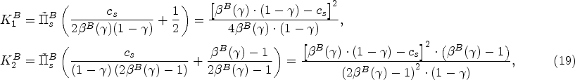
To begin, recall from Lemma 1 that, for any given store R’s price $p_r$ , store S’s gross profit ${\tilde{\mathrm{\Pi }}}_s^A(p_r)$ given in (10) (Figure 2(a)) is increasing in $p_r$ . Then, note that store S’s entry condition is: ${\tilde{\mathrm{\Pi }}}_s^A(p_r)\ge k$ (so that store S’s net profit ${\mathrm{\Pi }}_s^A(p_r)=(1-\gamma )\cdot [{\tilde{\mathrm{\Pi }}}_s^A(p_r)-k]\ge 0$ ). These two observations imply that there exists a threshold ${\tau }^A$ that solves ${\tilde{\mathrm{\Pi }}}_s^A({\tau }^A)=k$ in the following lemma so that store S’s entry condition holds (i.e., ${\tilde{\mathrm{\Pi }}}_s^A(p_r)\ge k$ ) if and only if $p_r\ge {\tau }^A$ ( the blue box in Figure 1). Before we present the expression for ${\tau }^A$ , let us define two terms for ease of exposition. Let

$$\begin{array}{rl}{K}_1^A& \equiv {\tilde{\mathrm{\Pi }}}_s^A\left(\frac{{\beta }^A(\gamma )+c_s}{2{\beta }^A(\gamma )}\right)=\frac{({\beta }^A(\gamma )-c_s{)}^2}{4{\beta }^A(\gamma )},\\ K_2^A& \equiv {\tilde{\mathrm{\Pi }}}_s^A\left(\frac{{\beta }^A(\gamma )-1+c_s}{2{\beta }^A(\gamma )-1}\right)=\frac{({\beta }^A(\gamma )-c_s{)}^2({\beta }^A(\gamma )-1)}{(2{\beta }^A(\gamma )-1{)}^2},\end{array}$$

(11)

where $K_1^A\ge K_2^A$ as depicted in Figure 2(a).

Lemma 2

In period 1, store R can deter store S’s entry by setting $p_r<{\tau }^A$ or tolerate store S’s entry by setting $p_r\ge {\tau }^A,$ where:

$${\tau }^A=\{\begin{array}{ll}\sqrt{4k({\beta }^A(\gamma )-1)}+c_s+1-{\beta }^A(\gamma )& k\le K_2^A,\\ {\displaystyle \frac{c_s+{\beta }^A(\gamma )-\sqrt{({\beta }^A(\gamma )-c_s{)}^2-4k{\beta }^A(\gamma )}}{2{\beta }^A(\gamma )}}& k\in (K_2^A,K_1^A],\\ \mathrm{\infty }& k>K_1^A.\end{array}$$

(12)

Lemma 2 implies that store S’s entry condition ${\tilde{\mathrm{\Pi }}}_s^A(p_r)\ge k$ (or equivalently, ${\mathrm{\Pi }}_s^A(p_r)\ge 0$ ) is equivalent to the condition $p_r\ge {\tau }^A$ . Hence, if store R aims to deter, it can afford to do so when its unit cost $c_r<{\tau }^A$ . Hence, store R’s problem (8) can be simplified as:

$${\mathrm{\Pi }}_r^{d,A}=\underset{p_r\in [c_r,{\tau }^A)}{sup}(p_r-c_r)\cdot (1-p_r).$$

(13)

On the other hand, if store R aims to tolerate store S’s entry, it sets a price $p_r\ge {\tau }^A$ (with ${\tau }^A>c_s+1-{\beta }^A(\gamma )$ as observed from Lemma 2). In this case, by using the consumer demand $q_r^A$ for store R as stated Corollary 1, store R’s problem (9) can be simplified as:

$$\begin{array}{rl}& {\mathrm{\Pi }}_r^{t,A}=\underset{p_r\ge max\{c_r,{\tau }^A\}}{max}(p_r-c_r)\cdot q_r^A,\\ & \text{s.t. }\\ & q_r^A=\{\begin{array}{ll}0& \text{if}{p}_r\ge \frac{{\beta }^A(\gamma )-1+c_s}{2{\beta }^A(\gamma )-1},\\ \frac{{\beta }^A(\gamma )-1+c_s-(2{\beta }^A(\gamma )-1)p_r}{2({\beta }^A(\gamma )-1)}& \text{if}{p}_r\in (c_s+1-{\beta }^A(\gamma ),\frac{{\beta }^A(\gamma )-1+c_s}{2{\beta }^A(\gamma )-1}).\end{array}\end{array}$$

(14)

By solving problems (13) and (14), we can identify store R’s deterrence strategy: deter store S’s entry by setting a price $p_r$ below ${\tau }^A$ if ${\mathrm{\Pi }}_r^{d,A}>{\mathrm{\Pi }}_r^{t,A}$ , and tolerate it; otherwise. Hence, we can determine store R’s equilibrium deterrence strategy and its equilibrium retail price $p_r^A$ that yields:

$${\mathrm{\Pi }}_r^A(p_r^A)=\underset{p_r\ge c_r}{max}\{{\mathrm{\Pi }}_r^{d,A},{\mathrm{\Pi }}_r^{t,A}\}.$$

(15)

4.2.2. Store R’s Deterrence Strategy: Cost Advantage $\alpha$

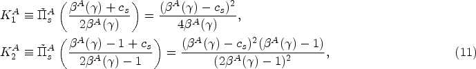
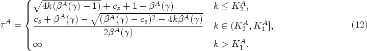
We now determine store R’s deterrence strategy by solving problem (15) that hinges upon store S’s entry cost $k$ and store R’s cost advantage $\alpha \equiv c_r/c_s<1$ . (As explained in Section 3, store R has a higher cost advantage when $\alpha$ is smaller.) In preparation, we define ${\mathrm{\Theta }}_1^A(k)$ and ${\mathrm{\Theta }}_2^A(k)$ as two thresholds for the cost advantage $\alpha$ so that ⁹ :

$$\begin{array}{rl}{\mathrm{\Theta }}_1^A(k)& =\{\begin{array}{ll}\frac{c_s+{\beta }^A(\gamma )-\sqrt{{({\beta }^A(\gamma )-c_s)}^2-4k\cdot {\beta }^A(\gamma )}}{2{\beta }^A(\gamma )\cdot c_s}& k\in (K_2^A,K_1^A],\\ \frac{c_s(4{\beta }^A(\gamma )-3)+({\beta }^A(\gamma )-1)\cdot [1-4{\beta }^A(\gamma )+8\sqrt{k({\beta }^A(\gamma )-1)}+4\sqrt{k((({\beta }^A(\gamma )-c_s)/(\sqrt{k({\beta }^A(\gamma )-1))})-2)}]}{c_s(2{\beta }^A(\gamma )-1)}& k\le K_2^A,\end{array}\end{array}$$

(16)

$$\begin{array}{rl}{\mathrm{\Theta }}_2^A(k)& =\{\begin{array}{ll}\frac{c_s+{\beta }^A(\gamma )-\sqrt{{({\beta }^A(\gamma )-c_s)}^2-4k{\beta }^A(\gamma )}}{2{\beta }^A(\gamma )\cdot c_s}& k\in (K_2^A,K_1^A],\\ \frac{{\beta }^A(\gamma )-1+c_s}{(2{\beta }^A(\gamma )-1)\cdot c_s}& k\le K_2^A.\end{array}\end{array}$$

(17)

Proposition 2

When facing a type (A) store S’s potential entry, store R’s deterrence strategy can be described as follows:

High entry cost: $k>K_1^A$ . Suppose store S’s entry cost $k>K_1^A$ . Then store S cannot afford to enter the market and store R can operate as a monopoly.

Medium entry cost: $k\in (K_2^A,K_1^A]$ . Suppose store S’s entry cost $k\in (K_2^A,K_1^A]$ . Then:

• (a)

If store R’s cost advantage is high (as $\alpha <{\mathrm{\Theta }}_1^A(k)={\mathrm{\Theta }}_2^A(k)$ ), then store R should deter store S’s entry. ¹⁰

(b)

If store R’s cost advantage is low (as $\alpha \ge {\mathrm{\Theta }}_2^A(k)={\mathrm{\Theta }}_1^A(k)$ ), then store R cannot deter the inevitable entry of store S. ¹¹

Low entry cost: $k\in (0,K_2^A]$ . Suppose store S’s entry cost $k\in (0,K_2^A]$ . Then:

• (a)

If store R’s cost advantage is high (as $\alpha <{\mathrm{\Theta }}_1^A(k)$ ), then store R should deter store S’s entry. ¹²

(b)

If store R’s cost advantage is medium (as $\alpha \in [{\mathrm{\Theta }}_1^A(k),{\mathrm{\Theta }}_2^A(k))$ ), then it is optimal for store R to tolerate store S’s entry. ¹³

(c)

If store R’s cost advantage is low (as $\alpha \ge {\mathrm{\Theta }}_2^A(k)$ ), then store R cannot deter the inevitable entry of store S. ¹⁴

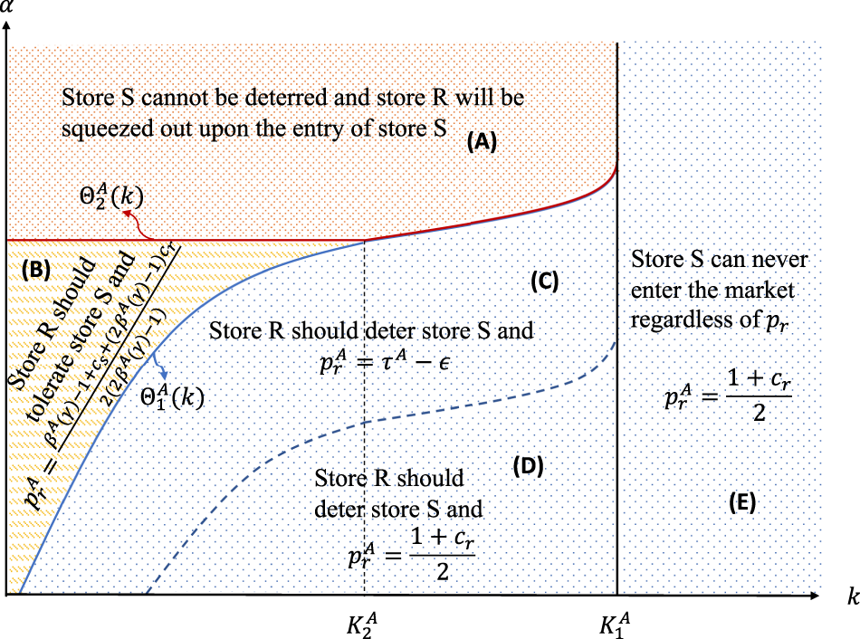
To interpret Proposition 2, we map out store R’s equilibrium deterrence strategy as stated in Proposition 2 based on store S’s entry cost $k$ and store R’s cost advantage factor $\alpha$ in Figure 3.

Figure 3.

Store R’s deterrence strategy in terms of store S’s entry cost $k$ and store R’s cost advantage $\alpha$ .

First, when store S’s entry cost is high: $k>K_1^A$ , statement 1 of Proposition 2 is depicted in zone (E) in Figure 3, highlighting the market condition is untenable for store S to enter.

Second, when store S’s entry cost is medium: $k\in (K_2^A,K_1^A]$ , store S’s potential entry is plausible. As such, store R’s deterrence strategy hinges upon its cost advantage over store S via  $\alpha$ . Specifically, when store R’s cost advantage over store S is sufficiently high (as $\alpha <{\mathrm{\Theta }}_1^A(k)$ ), store R can afford to deter store S’s entry as stated in statement 2(a) of Proposition 2 and depicted in zones (C) and (D) within the range $k\in (K_2^A,K_1^A]$ . However, when store R’s cost advantage over store S is low (as $\alpha \ge {\mathrm{\Theta }}_1^A(k)$ ), store R cannot afford to deter store S’s entry as depicted in zone (A) within the range $k\in (K_2^A,K_1^A]$ .

Third, when store S’s entry cost is low: $k\le K_2^A$ , store S’s potential entry is now imminent. Specifically, the zones (C), (D), and (A) within the range $k\in (0,K_2^A]$ as depicted in Figure 3 are based on statements 3(a) and 3(c), and they can be interpreted in the same manner as above. Interestingly, there is a new zone (B) corresponding to statement 3(b) that deserves our attention. Specifically, when store S’s entry cost is low, store R should tolerate store S’s entry when its cost advantage is medium, even if it can profitably deter store S’s entry. Faced with the threat from store S, the incumbent store R faces a trade-off between the loss of profit due to charging a lower deterrence price or the loss of profit due to losing some of its market share to store S. In zone (B), the incumbent store R can be “better off” by tolerating store S’s entry and sharing the market with it, rather than lowering the price to a very low level to deter store S’s entry.

By substituting the equilibrium price $p_r^A$ given by Proposition 2 for different regions of $(k,\alpha )$ into Proposition 1 and Corollary 1, we can derive store S’s equilibrium price $p_s^A$ , equilibrium profit ${\tilde{\mathrm{\Pi }}}_s^A$ , and demand $q_s^A$ (and store R’s demand $q_r^A$ ). Because our focus is on the deterrence strategy, we shall omit these tedious expressions under different conditions.

In summary, our analytical results formalize our understanding regarding how a type (A) store S’s entry cost $k$ and store R’s cost advantage $\alpha$ affect store R’s deterrence strategy as stated in Proposition 2 and Figure 3. How would these results change if the potential entrant is a type (B) store S who donates a proportion of its revenue (instead of profit) to charity? We shall examine this question next.

5. Market-Entry Game Between a Type (B) Store S and an Incumbent Store R

We now use the same approach as before to examine the market-entry game between store R and a type (B) store S donates a proportion $\gamma$ of its revenue (instead of profit), creating the warm-glow effect ${\beta }^B(\gamma )$ . Recognizing this difference, we characterize a type (B) store S’s best-response pricing strategy in Section 5.1, followed by store R’s deterrence strategy in Section 5.2.

5.1. Type (B) Store S’s Best-Response Pricing Strategy in Period 2

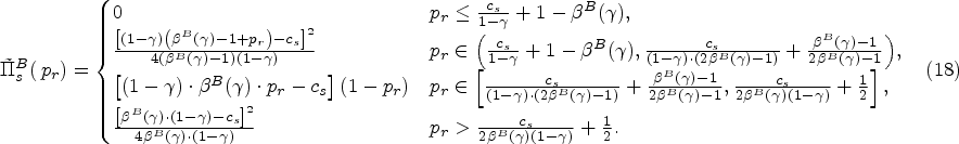
Given store R’s retail price $p_r$ , a type (B) store S determines its best-response price $p_s^B(p_r)$ by solving (7). Before we present $p_s^B(p_r)$ as stated in Proposition 3, let us first rewrite the effective maximum profit given in (7) as: ${\mathrm{\Pi }}_s^B(p_r)=(1-\gamma )p_s^B{q}_s^B-c_s{q}_s^B-k={\tilde{\mathrm{\Pi }}}_s^B-k$ , where ${\tilde{\mathrm{\Pi }}}_s^B\equiv ((1-\gamma )p_s^B-c_s)\cdot q_s^B$ represents the maximum gross profit without considering the entry cost $k$ . Hence, a type (B) store S can enter the market if and only if ${\tilde{\mathrm{\Pi }}}_s^B\ge k$ (or equivalently, ${\mathrm{\Pi }}_s^B(p_r)\ge 0$ ). By solving (7), we get:

Lemma 3

Given any store R’s price $p_r$ , a type (B) store S’s gross profit ${\tilde{\mathrm{\Pi }}}_s^B(p_r)$ satisfies:

$$\begin{array}{rl}& {\tilde{\mathrm{\Pi }}}_s^B(p_r)=\{\begin{array}{ll}0& p_r\le \frac{c_s}{1-\gamma }+1-{\beta }^B(\gamma ),\\ \frac{{[(1-\gamma )({\beta }^B(\gamma )-1+p_r)-c_s]}^2}{4({\beta }^B(\gamma )-1)(1-\gamma )}& p_r\in (\frac{c_s}{1-\gamma }+1-{\beta }^B(\gamma ),\frac{c_s}{(1-\gamma )\cdot (2{\beta }^B(\gamma )-1)}+\frac{{\beta }^B(\gamma )-1}{2{\beta }^B(\gamma )-1}),\\ [(1-\gamma )\cdot {\beta }^B(\gamma )\cdot p_r-c_s](1-p_r)& p_r\in [\frac{c_s}{(1-\gamma )\cdot (2{\beta }^B(\gamma )-1)}+\frac{{\beta }^B(\gamma )-1}{2{\beta }^B(\gamma )-1},\frac{c_s}{2{\beta }^B(\gamma )(1-\gamma )}+\frac{1}{2}],\\ \frac{{[{\beta }^B(\gamma )\cdot (1-\gamma )-c_s]}^2}{4{\beta }^B(\gamma )\cdot (1-\gamma )}& p_r>\frac{c_s}{2{\beta }^B(\gamma )(1-\gamma )}+\frac{1}{2}.\end{array}\end{array}$$

(18)

Also, ${\tilde{\mathrm{\Pi }}}_s^B(p_r)$ is nondecreasing in $p_r$ .

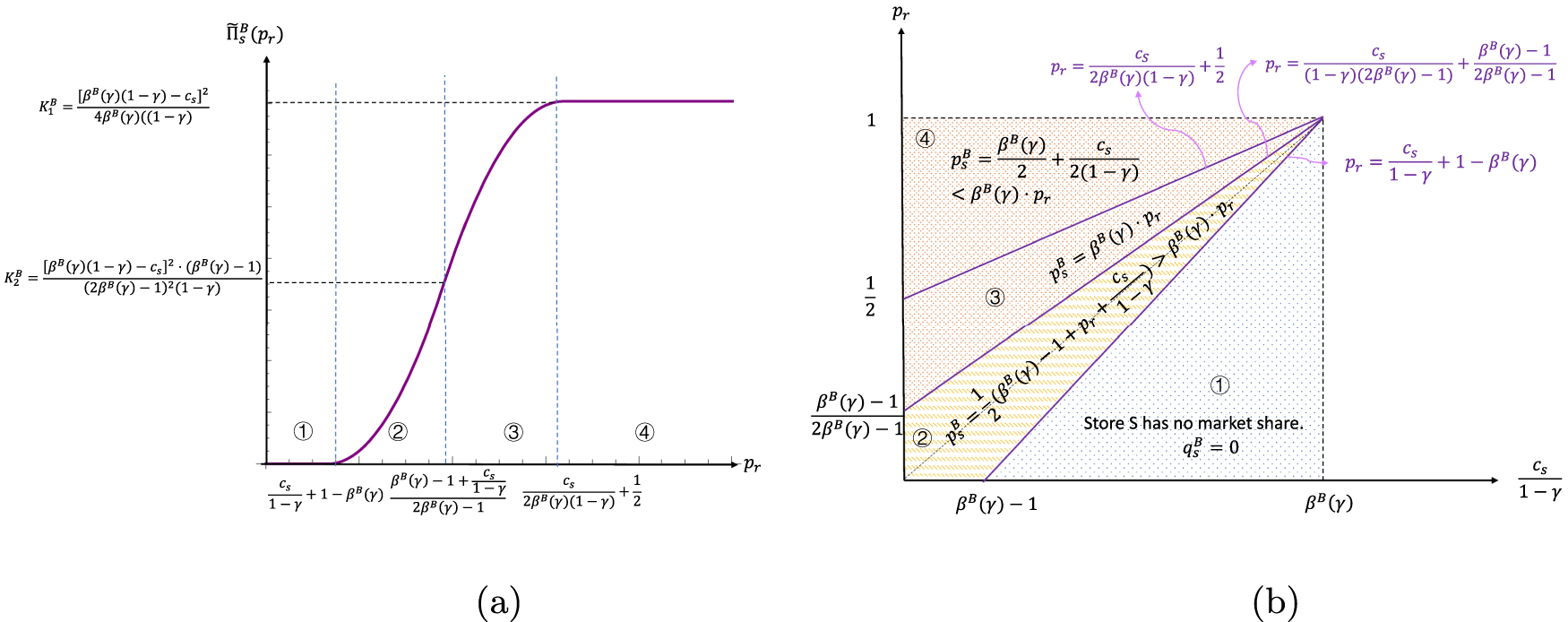
We illustrate the gross profit ${\tilde{\mathrm{\Pi }}}_s^B(p_r)$ in Figure 4(a) that resembles Figure 2(a) in Section 4.1, and it has the same interpretation. Also, observe from Lemma 3 that store S’s entry condition is violated if store R set $p_r$ sufficiently low so that $p_r\le (c_s/(1-\gamma ))+1-{\beta }^B(\gamma )$ . By ruling out this trivial case, we get:

Figure 4.

Type (B) store S’s best-response pricing strategy: (a) type (B) store S’s gross profit ${\tilde{\mathrm{\Pi }}}_s^B(p_r)$ and (b) type (B) store S’s best-response price $p_s^B$ .

Proposition 3

Suppose store R sets its price at $p_r$ that satisfies $p_r>(c_s/(1-\gamma ))+1-{\beta }^B(\gamma )$ and store S’s entry condition $k\le {\tilde{\mathrm{\Pi }}}_s^B(p_r)$ holds, where ${\tilde{\mathrm{\Pi }}}_s^B(p_r)$ is given in Lemma 3. Then a type (B) store S’s best-response price $p_s^B$ , consumer demand $q_s^B$ , and its retained profit ${\mathrm{\Pi }}_s^B={\tilde{\mathrm{\Pi }}}_s^B-k$ satisfy:

• (i)

If $p_r\in (\frac{c_s}{1-\gamma }+1-{\beta }^B(\gamma ),\frac{c_s}{(1-\gamma )\cdot (2{\beta }^B(\gamma )-1)}+\frac{{\beta }^B(\gamma )-1}{2{\beta }^B(\gamma )-1})$ , then the best-response $p_s^B=\frac{1}{2}({\beta }^B(\gamma )-1+p_r+\frac{c_s}{1-\gamma })>{\beta }^B(\gamma )\cdot p_r$ , so the corresponding $q_s^B=\frac{{\beta }^B(\gamma )-1+p_r}{2({\beta }^B(\gamma )-1)}-\frac{c_s}{2(1-\gamma )\cdot ({\beta }^B(\gamma )-1)}$ and ${\mathrm{\Pi }}_s^B=\frac{[(1-\gamma )({\beta }^B(\gamma )-1+p_r)-c_s{]}^2}{4({\beta }^B(\gamma )-1)(1-\gamma )}-k$ .

(ii)

If $p_r\in [\frac{c_s}{(1-\gamma )(2{\beta }^B(\gamma )-1)}+\frac{{\beta }^B(\gamma )-1}{2{\beta }^B(\gamma )-1},\frac{c_s}{2{\beta }^B(\gamma )\cdot (1-\gamma )}+\frac{1}{2}]$ , then the best-response $p_s^B={\beta }^B(\gamma )\cdot p_r$ , so the corresponding $q_s^B=1-p_r$ and ${\mathrm{\Pi }}_s^B=[(1-\gamma )\cdot {\beta }^B(\gamma )\cdot p_r-c_s]\cdot (1-p_r)-k$ .

(iii)

If $p_r>\frac{c_s}{2{\beta }^B(\gamma )\cdot (1-\gamma )}+\frac{1}{2}$ , then the best-response $p_s^B=\frac{{\beta }^B(\gamma )}{2}+\frac{c_s}{/}2(1-\gamma )<{\beta }^B(\gamma )\cdot p_r$ , so the corresponding $q_s^B=\frac{1}{2}-\frac{c_s}{2{\beta }^B(\gamma )\cdot (1-\gamma )}$ , and ${\mathrm{\Pi }}_s^B=\frac{[{\beta }^B(\gamma )(1-\gamma )-c_s{]}^2}{4{\beta }^B(\gamma )\cdot (1-\gamma )}-k$ .

Observe that Lemma 3 and Proposition 3 illustrated in Figure 4 resemble Lemma 1 and Proposition 1 depicted in Figure 2. Next, by substituting $p_s^B(p_r)$ stated in Proposition 3 into (3) and (4), we can derive the consumer demand for store R upon the entry of a type (B) store S as follows.

Corollary 2

When $p_r>(c_s/(1-\gamma ))+1-{\beta }^B(\gamma )$ and $k\le {\tilde{\mathrm{\Pi }}}_s^B(p_r)$ , the demand for each store upon the entry of a type (B) store S depends on $p_r$ as follows.

• (i)

When $p_r\in ((c_s/(1-\gamma ))+1-{\beta }^B(\gamma ),(c_s/((1-\gamma )(2{\beta }^B(\gamma )-1)))+(({\beta }^B(\gamma )-1)/(2{\beta }^B(\gamma )-1)))$ , store R’s demand $q_r^B=(({\beta }^B(\gamma )-1-(2{\beta }^B(\gamma )-1)\cdot p_r)/(2({\beta }^B(\gamma )-1)))+(c_s/(2(1-\gamma )\cdot ({\beta }^B(\gamma )-1)))$ , which is increasing in $c_s$ and decreasing in $p_r$ . Also, the corresponding store S’s demand $q_s^B$ as given in (i) of Proposition 3 is increasing in $p_r$ and decreasing in $c_s$ .

(ii)

When $p_r\ge (c_s/((1-\gamma )\cdot (2{\beta }^B(\gamma )-1)))+(({\beta }^B(\gamma )-1)/(2{\beta }^B(\gamma )-1))$ , store R’s demand $q_r^B=0$ and store S’s demand $q_s^B$ as given in (ii) and (iii) of Proposition 3 is nonincreasing in $p_r$ and $c_s$ .

5.2. Store R’s Equilibrium Deterrence Strategy in Period 1

By anticipating store (B)’s best response as stated in Proposition 3, we now characterize store R’s deterrence strategy (by using the same approach as stated in Section 4.2).

5.2.1. Store R’s Deterrence Price Threshold ${\tau }^B$

To begin, we characterize the deterrence threshold for $p_r$ (denoted as ${\tau }^B$ ) in Lemma 4 so that store R can deter a type (B) store S’s entry by choosing a retail price $p_r<{\tau }^B$ or tolerate its entry by setting $p_r\ge {\tau }^B$ . Analogous to thresholds $K_1^A$ and $K_2^A$ as defined in Section 4.2, let:

$$\begin{array}{rl}{K}_1^B& ={\tilde{\mathrm{\Pi }}}_s^B(\frac{c_s}{2{\beta }^B(\gamma )(1-\gamma )}+\frac{1}{2})=\frac{{[{\beta }^B(\gamma )\cdot (1-\gamma )-c_s]}^2}{4{\beta }^B(\gamma )\cdot (1-\gamma )},\\ K_2^B& ={\tilde{\mathrm{\Pi }}}_s^B(\frac{c_s}{(1-\gamma )(2{\beta }^B(\gamma )-1)}+\frac{{\beta }^B(\gamma )-1}{2{\beta }^B(\gamma )-1})=\frac{{[{\beta }^B(\gamma )\cdot (1-\gamma )-c_s]}^2\cdot ({\beta }^B(\gamma )-1)}{{(2{\beta }^B(\gamma )-1)}^2\cdot (1-\gamma )},\end{array}$$

(19)

where $K_1^B\ge K_2^B$ . Observe from Proposition 3 and Figure 4(a) that a type (B) store S can never enter the market when its entry cost $k>K_1^B$ regardless of the value of $p_r$ (i.e., ${\tau }^B=\mathrm{\infty }$ ). Hence, it suffices to focus on the case when $k\le K_1^B$ by focusing on the deterrence threshold ${\tau }^B$ as follows.

Lemma 4

Store R can either deter a type (B) store’s entry by setting $p_r<{\tau }^B$ , or tolerate its entry by setting $p_r\ge {\tau }^B$ , where:

$${\tau }^B=\{\begin{array}{ll}\frac{\sqrt{4k({\beta }^B(\gamma )-1)\cdot (1-\gamma )}+c_s}{1-\gamma }+1-{\beta }^B(\gamma )& k\le K_2^B,\\ \frac{\begin{array}{c}{c}_s+{\beta }^B(\gamma )\cdot (1-\gamma )-\sqrt{{[{\beta }^B(\gamma )\cdot (1-\gamma )-c_s]}^2-4k{\beta }^B(\gamma )\cdot (1-\gamma )}\end{array}}{2{\beta }^B(\gamma )\cdot (1-\gamma )}& k\in (K_2^B,K_1^B],\\ \mathrm{\infty }& k>K_1^B,\end{array}$$

(20)

Applying Lemma 4 in the same way as in Section 4.2.1, we can examine type (B) store S’s entry condition (i.e., ${\tilde{\mathrm{\Pi }}}_s^B(p_r)\ge k$ ) from store R’s perspective; that is, $p_r\ge {\tau }^B$ . Hence, we can simplify store R’s problem (8) under deterrence that is analogous to (13) and obtain store R’s corresponding profit ${\mathrm{\Pi }}_r^{d,B}$ . We can also simplify store R’s problem (9) under tolerance that is analogous to (14) and obtain store R’s corresponding profit ${\mathrm{\Pi }}_r^{t,B}$ . To avoid repetition, we omit the details.

5.2.2. Store R’s Deterrence Strategy: Cost Advantage $\alpha$

Once we determine store R’s profit ${\mathrm{\Pi }}_r^{d,B}$ (or ${\mathrm{\Pi }}_r^{t,B}$ ) when it chooses to deter (or tolerate) store S’s entry, we can determine store R’s deterrence strategy by comparing these two quantities as explained in Section 3.2.4. Before we characterize store R’s equilibrium deterrence strategy in Proposition 4, let us recall from Section 4.2 that store R’s deterrence strategy is based on its cost competitiveness measured by $\alpha$ (because $c_r=\alpha \cdot c_s$ ) and store S’s entry cost $k$ . Analogous to the thresholds ${\mathrm{\Theta }}_1^A(k)$ and ${\mathrm{\Theta }}_2^A(k)$ as defined in Section 4.2, we define two thresholds for store R’s cost advantage $\alpha =c_r/c_s$ .

Let:

$$\begin{array}{rl}{\mathrm{\Theta }}_1^B(k)& =\{\begin{array}{ll}\frac{c_s+{\beta }^B(\gamma )(1-\gamma )-\sqrt{{[{\beta }^B(\gamma )\cdot (1-\gamma )-c_s]}^2-4k{\beta }^B(\gamma )\cdot (1-\gamma )}}{2{\beta }^B(\gamma )\cdot (1-\gamma )c_s}& k\in (K_2^B,K_1^B],\\ \frac{c_s(4{\beta }^B(\gamma )-3)+({\beta }^B(\gamma )-1)\cdot [1-\gamma -4{\beta }^B(\gamma )\cdot (1-\gamma )+8\sqrt{k({\beta }^B(\gamma )-1)\cdot (1-\gamma )}+4\sqrt{k(1-\gamma )((({\beta }^B(\gamma )\cdot (1-\gamma )-c_s)/(\sqrt{k({\beta }^B(\gamma )-1)(1-\gamma )}))-2)}]}{c_s(2{\beta }^B(\gamma )-1)(1-\gamma )}& k\le K_2^B.\end{array}\end{array}$$

(21)

$$\begin{array}{rl}{\mathrm{\Theta }}_2^B(k)& =\{\begin{array}{ll}\frac{c_s+{\beta }^B(\gamma )(1-\gamma )-\sqrt{{[{\beta }^B(\gamma )\cdot (1-\gamma )-c_s]}^2-4k{\beta }^B(\gamma )\cdot (1-\gamma )}}{2{\beta }^B(\gamma )\cdot (1-\gamma )c_s}& k\in (K_2^B,K_1^B],\\ \frac{{\beta }^B(\gamma )-1}{(2{\beta }^B(\gamma )-1)\cdot c_s}+\frac{1}{(2{\beta }^B(\gamma )-1)(1-\gamma )}& k\le K_2^B.\end{array}\end{array}$$

(22)

Proposition 4

When facing the potential entry of a type (B) store S, store R’s deterrence strategy can be described as follows:

High entry cost: $k>K_1^B$ . Suppose a type (B) store S’s entry cost $k>K_1^B$ . Then store S cannot afford to enter the market and store R can operate as a monopoly.

Medium entry cost: $k\in (K_2^B,K_1^B]$ . Suppose a type (B) store S’s entry cost $k\in (K_2^B,K_1^B]$ . Then:

If store R’s cost advantage is high (as $\alpha <{\mathrm{\Theta }}_1^B(k)={\mathrm{\Theta }}_2^B(k)$ ), then store R should deter store S’s entry. ¹⁵

If store R’s cost advantage is low (as $\alpha \ge {\mathrm{\Theta }}_2^B(k)={\mathrm{\Theta }}_1^B(k)$ ), then store R cannot deter the inevitable entry of store S. ¹⁶

Low entry cost: $k\in (0,K_2^B]$ . Suppose store S’s entry cost $k\in (0,K_2^B]$ . Then:

If store R’s cost advantage is high (as $\alpha <{\mathrm{\Theta }}_1^B(k)$ ), then store R should deter store S’s entry. ¹⁷

If store R’s cost advantage is medium (as $\alpha \in [{\mathrm{\Theta }}_1^B(k),{\mathrm{\Theta }}_2^B(k))$ ), then it is optimal for store R to tolerate store S’s entry. ¹⁸

If store R’s cost advantage is low (as $\alpha \ge {\mathrm{\Theta }}_2^B(k)$ ), then store R cannot deter the inevitable entry of store S. ¹⁹

Proposition 4 shows that the deterrence strategy for store R against a type (B) store S’s entry possesses the same structure as that against a type (A) store S (see Proposition 2 and Figure 3). As such, it can be interpreted in the same manner as in Section 4.2.2. We omit the details.

6. Store R’s Deterrence Strategies Across Different Types of Store S

While store R’s deterrence strategies against both types of store S follow the same structure as presented in Proposition 2 (for type (A)) and Proposition 4 (for type (B)), store R may be more willing to tolerate or deter the entry of one type than the other types. This is because, as shown in Propositions 2 and 4, store R’s deterrence strategy depends on those thresholds $K_1^j$ and $K_2^j$ for type $j$ store S entry cost given in (11) and (19), and those thresholds ${\mathrm{\Theta }}_1^j(k)$ and ${\mathrm{\Theta }}_2^j(k)$ for store R’s cost advantage $\alpha$ given in (16), (17), (21), and (22). Also, observe from (16), (17), (21), and (22) that these thresholds depend on those type-specific pre-committed donating proportions ${\gamma }^A$ and ${\gamma }^B$ along with those warm-glow effects ${\beta }^A({\gamma }^A)$ and ${\beta }^B({\gamma }^B)$ .

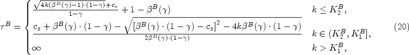
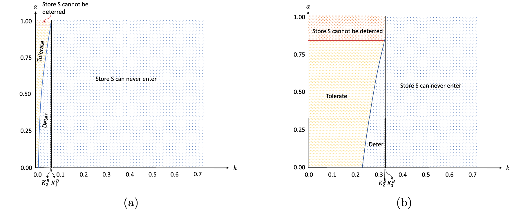
These observations motivate us to compare store R’s deterrence strategies when facing two different types of store S’s entry for the case when both types of stores generate the same level of warm-glow effect ${\beta }^A({\gamma }^A)={\beta }^B({\gamma }^B)$ even though the proportions ${\gamma }^A\ne {\gamma }^B$ . Before we conduct the comparison analytically, we first use Figure 5 to numerically illustrate store R’s optimal deterrence strategies against two types of store S by setting $c_s=0.8$ , ${\gamma }^A=0.1$ , and ${\gamma }^B=0.05$ . While ${\gamma }^A>{\gamma }^B$ in this example, we consider a linear warm-glow effect. Specifically, we set ${\beta }^A({\gamma }^A)=1+b^A\cdot {\gamma }^A=1+5\cdot {\gamma }^A=1.5$ and ${\beta }^B({\gamma }^B)=1+b^B\cdot {\gamma }^B=1+10\cdot {\gamma }^B=1.5$ so that ${\beta }^A({\gamma }^A)={\beta }^B({\gamma }^B)$ .

Figure 5.

Store R’s equilibrium deterrence strategy against both types of store S (setting: $c_s=0.8$ , ${\gamma }^A=0.1$ , ${\gamma }^B=0.05$ , ${\beta }^A({\gamma }^A)=1+5\cdot {\gamma }^A=1.5$ , and ${\beta }^B({\gamma }^B)=1+10\cdot {\gamma }^B=1.5$ ): (a) deterrence strategy against type (A) store S and (b) deterrence strategy against type (B) store S.

First, let us examine the entry conditions for both types of store S through $K_1^j$ and $K_2^j$ ; that is, the thresholds with respect to the entry cost $k$ of a type $j$ store, $j=A,B$ . Observe from Figure 5(a) and (b) that, because $K_1^B<K_1^A$ , the (blue) area $k>K_1^B$ is larger than the (blue) area $k>K_1^A$ so that a type (B) store will find it more difficult to enter the market relative to a type (A) store. More formally, when the entry cost $k\in [K_1^B,K_1^A)$ for both types of store S, a type (B) store S cannot afford to enter the market (because $k>K_1^B$ as stated in statement 1 of Proposition 4) even though a type (A) store S may be able to do so (because $k<K_1^A$ as stated in Proposition 2). Hence, from store S’s vantage point of entry cost $k$ , a type (B) store S is less affordable to enter the market than a type (A) store S.

Second, let us examine the thresholds ${\mathrm{\Theta }}_2^j(k)$ in relation to store R’s cost advantage $\alpha =c_r/c_s<1$ . As shown in Figure 5(a) and (b), ${\mathrm{\Theta }}_2^B(k)>{\mathrm{\Theta }}_2^A(k)$ , which implies that the (pink) area $\alpha >{\mathrm{\Theta }}_2^A(k)$ is larger than the (pink) area $\alpha >{\mathrm{\Theta }}_2^B(k)$ . To be more precise, when store R’s cost advantage $\alpha \in ({\mathrm{\Theta }}_2^A(k),{\mathrm{\Theta }}_2^B(k)]$ for both types of store S, store R cannot deter the type (A) store S’s entry (because $\alpha \ge {\mathrm{\Theta }}_2^A(k)$ as stated in statements 2(b) and 3(c) of Proposition 2); however, store R can deter the type (B) store S’s entry (because $\alpha <{\mathrm{\Theta }}_2^B(k)$ as stated in statements 2(a), 3(a) and 3(b) of Proposition 4). Hence, from store R’s vantage point of its cost advantage $\alpha$ , it is relatively easier for store R to deter a type (B) store than a type (A) store.

Third, observe from Figure 5(a) and (b) that $K_2^B<K_2^A$ and ${\mathrm{\Theta }}_1^A(k)<{\mathrm{\Theta }}_1^B(k)$ . Thus, when $k<K_2^B<K_2^A$ , $\alpha \in ({\mathrm{\Theta }}_1^A(k),{\mathrm{\Theta }}_2^A(k)]$ and $\alpha <{\mathrm{\Theta }}_1^B(k)$ , store R would deter a type (B) store, but tolerate the entry of a type (A) store. In Figure 5, it can be observed that the (blue) area (in which store R will deter and/or store S cannot enter) is larger for a type (B) store than that of a type (A) store, whereas the (yellow and pink) area (in which store S can enter) is larger for a type (A) store S than that of a type (B) store S. This implies that store R tends to take a more aggressive deterrence strategy against the entry of a type (B) store S than a type (A) store S.

To conclude, the numerical example shown in Figure 5 suggests that the incumbent store R is more aggressive in deterring a type (B) than a type (A) store S, and it is relatively easier for a type (A) store S to enter the market. However, is this result always true? Due to the complexity of the expressions for the thresholds mentioned earlier, it becomes analytically intractable to analyze a general case where the proportion ${\gamma }^j$ is endogenously determined by each type of store S. Therefore, in order to establish a hypothesis, we focus on analytically examining a benchmark case where both stores generate an identical warm-glow effect (i.e., ${\beta }^A({\gamma }^A)={\beta }^B({\gamma }^B)$ ) in Section 6 (also note that the pre-committed donating proportions of two types of store S can be different, i.e., ${\gamma }^A\ne {\gamma }^B$ ). We shall numerically examine this hypothesis by considering the case where ${\gamma }^j$ is endogenously determined by each type $j$ of store S in Section 7 so that the donation proportion along with the warm-glow effect generated by store S will become type-specific; that is, ${\gamma }^A\ne {\gamma }^B$ and ${\beta }^A({\gamma }^A)\ne {\beta }^B({\gamma }^B)$ .

6.1. Best-Response Pricing Strategies for Type (A) and Type (B) Store S

First, by comparing the results given in Propositions 1 and 3 together with Corollaries 1 and 2, we obtain Corollary 3 that compares entry conditions, best-response pricing strategies, and consumer demand for type (A) and type (B) store S.

Corollary 3

Suppose both types of store S generate the same level of warm-glow effect (i.e., ${\beta }^A({\gamma }^A)={\beta }^B({\gamma }^B)$ ). Then, given store R’s price $p_r$ , the entry conditions and best-response prices for both types of store S, and the corresponding consumer demand satisfy:

Best-response pricing strategy comparison. A type (B) store S would charge a higher price than a type (A) S store upon entering the market; that is, $p_s^B\ge p_s^A$ .

Entry condition comparison. The entry condition for a type (A) store (i.e., ${\tilde{\mathrm{\Pi }}}_s^A\ge k$ ) is less stringent than that of type (B) because ${\tilde{\mathrm{\Pi }}}_s^A\ge {\tilde{\mathrm{\Pi }}}_s^B$ .

Consumer demand comparison. The consumer demand for a type (A) store is higher than that of a type (B) store; that is, $q_s^A\ge q_s^B$ . Accordingly, the consumer demand for store R is lower upon a type (A) store S’s entry than a type (B) store S’s entry; that is, $q_r^A\le q_r^B$ .

To motivate Corollary 3, let us consider a general case where the warm-glow effect ${\beta }^j({\gamma }^j)$ is store “type-specific” with $j=A,B$ . Suppose the donating proportion is the same so that ${\gamma }^A={\gamma }^B=\gamma$ . Then a type (B) store may generate a higher warm-glow effect than a type (A) store (i.e., ${\beta }^B(\gamma )>{\beta }^A(\gamma )$ ). This is because consumers have a stronger understanding of the direct relationship between their purchases and a type (B) store’s donation that is based on a proportion of its revenue. ²⁰ In this context, the warm-glow effect for a type (B) store would be higher. Consequently, a type (B) store can afford to set a lower proportion that has ${\gamma }^B<{\gamma }^A$ in order to create the same level of warm-glow effect ${\beta }^A({\gamma }^A)={\beta }^B({\gamma }^B)$ . The numerical study illustrated in Figure 5 provides an example of the case where $0.05={\gamma }^B<{\gamma }^A=0.1$ and ${\beta }^B({\gamma }^A)={\beta }^B({\gamma }^B)=1.5$ .

Corollary 3 examines the case when both types of store S generate the same level of warm-glow effect ${\beta }^A({\gamma }^A)={\beta }^B({\gamma }^B)$ (even though a type (B) store may donate a lower proportion, i.e., ${\gamma }^B<{\gamma }^A$ ). First, Corollary 3(a) implies that the best-response price set by a type (B) store S is higher than a type (A) store S, given that both types of store S generate the same level of warm-glow effect. In particular, this holds true even if a type (B) store S may contribute a much smaller proportion ${\gamma }^B$ compared to ${\gamma }^A$ from a type (A) store S. This is because a type (B) store donates its revenue (not profit as for a type (A) store). Consequently, a type (B) store S has to charge a higher price than a type (A) store S in order to cover its cost. Second, statement (b) states that it is easier for a type (A) store S to enter the market than a type (B) store S for the same entry cost $k$ because the gross profit ${\tilde{\mathrm{\Pi }}}_s^A\ge {\tilde{\mathrm{\Pi }}}_s^B$ . Finally, Corollary 3(c) implies that, from store R’s perspective, a type (A) store S poses a higher threat than a type (B) store S because the former can siphon off more demand from store R after entering the market than the latter. This is because a type (A) store S can afford to charge a lower price than a type (B) store S as shown in statement (a).

6.2. Store R’s Deterrence Strategies Against a Type (A) and Type (B) Store S

In view of the differences in terms of entry conditions, best-response price, and consumer demand across two types of stores as stated in Corollary 3, we now compare store R’s deterrence strategies across different types of store S in two ways. First, recall from Lemma 2 (Lemma 4) that store R can deter a type (A) (type (B)) store S by setting a price $p_r<{\tau }^A$ ( $p_r<{\tau }^B$ ). As such, by directly comparing ${\tau }^A$ and ${\tau }^B$ , we can derive the relative difficulty of deterring different types of store S. Second, because $\alpha =c_r/c_s<1$ captures store R’s cost advantage over store S and $k$ captures store S’s entry barrier, we can compare the store R’s deterrence strategies across different types of store S by comparing the corresponding thresholds for $\alpha$ and $k$ as presented in Propositions 2 and 4. The following corollary compares store R’s deterrence strategy across different types of store S.

Corollary 4

Suppose both types of store S generate the same level of warm-glow effect (i.e., ${\beta }^A({\gamma }^A)={\beta }^B({\gamma }^B)$ ). Then store R’s deterrence strategies across different types of store S satisfy:

The price deterrence thresholds. The price deterrence thresholds for store R’s retail price against two types of store S satisfy ${\tau }^A<{\tau }^B$ .

The cost deterrence thresholds. Store R’s deterrence strategies as stated in Propositions 2 and 4 hinge on whether $k$ lies within a certain region and whether $\alpha$ is above or below certain thresholds: $K_i^j$ and ${\mathrm{\Theta }}_i^j(k)$ , $i\in \{1,2\}$ and $j\in \{A,B\}$ . Specifically, these thresholds satisfy: $K_1^A>K_1^B$ , $K_2^A>K_2^B$ , ${\mathrm{\Theta }}_1^A(k)<{\mathrm{\Theta }}_1^B(k)$ , and ${\mathrm{\Theta }}_2^A(k)<{\mathrm{\Theta }}_2^B(k)$ .

Corollary 4 implies that, given that both types of store S generate the same level of warm-glow effect (i.e., ${\beta }^A({\gamma }^A)={\beta }^B({\gamma }^B)$ ), store R is more likely to deter a type (B) store S than a type (A) store S, even though a type (B) store S may donate a lower proportion ${\gamma }^B$ than ${\gamma }^A$ . Specifically, Corollary 4(a) indicates that, because ${\tau }^A<{\tau }^B$ , the condition for store R to deter a type (A) store S (i.e., $p_r<{\tau }^A$ ) is more “stringent” than that of type (B) (i.e., $p_r<{\tau }^B$ ). Hence, relatively speaking, it is more affordable for store R to deter a type (B) store S without setting a much lower price $p_r$ . Next, Corollary 4(b) demonstrates the same results as depicted in Figure 5.

To summarize, the analysis of the benchmark case, where two types of store S generate the same level of warm-glow effect (i.e., ${\beta }^A({\gamma }^A)={\beta }^B({\gamma }^B)$ ), indicates that the incumbent store R is more likely to deter a type (B) store S than a type (A) store S. The question remains whether this hypothesis holds true when $\gamma$ is determined endogenously by each type of store S. We will address this through numerical examination in Section 7.

7. Endogenously Determined Donating Proportion ${\gamma }^j$ for Store Type $j=A,B$

We now expand our analysis to the case when the donating proportion is “endogenously determined” by a type (A) (or (B)) store S. We consider a similar decision sequence described in Section 3.1. In period 1, store R chooses its price $p_r$ to either deter or tolerate store S’s entry; and if store R chooses to tolerate store S’s entry, then in period 2 a type $j$ store S determines its donating proportion ${\gamma }^j$ along with its price $p_s^j$ to compete with store R, where $j=A,B$ . Since the market-entry game is not analytically solvable when ${\gamma }^j$ is endogenously determined, we numerically search for the optimal ${\gamma }^j$ in the range of $(0,1)$ that maximizes the profit of a type $j$ store S. To capture the warm-glow effect ${\beta }^j({\gamma }^j)\ge 1$ is an increasing function of ${\gamma }^j$ (a decision variable for a type $j$ store S), we shall assume:

$${\beta }^j({\gamma }^j)=1+b^j\cdot ({\gamma }^j{)}^t,j\in \{A,B\},$$

(23)

where the parameters $t>0$ ²¹ and $b^j>0$ . In this section, we focus on the scenario where $t=1$ so that the warm-glow effect function given in (23) takes on a linear form. In the Online Appendix B, we present our results for the case when $t\ne 1$ so that ${\beta }^j({\gamma }^j)$ is a nonlinear function of ${\gamma }^j$ . Overall, we find similar structural results as presented earlier in Sections 4, 5, and 6.

7.1. Store R’s Deterrence Strategies Against Both Types Store S.

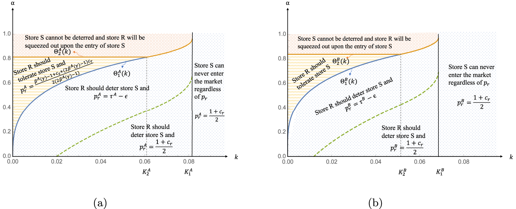
Because the key focus of the paper is to analyze store R’s deterrence strategies in response to store S’s entry, we begin by presenting our numerical results related to store R’s optimal deterrence strategy for the case when $\gamma$ is endogenously determined by each type of store S. Figures 6 and 7 depict store R’s optimal deterrence strategies against a type (A) and a type (B) store S, respectively.

Figure 6.

Store R’s equilibrium deterrence strategy against a type (A) store S. Setting: $c_s=0.7$ . (a) store R’s deterrence strategy against a type (A) store S with ${\beta }^A({\gamma }^A)=1+3\cdot {\gamma }^A$ and, (b) store R’s deterrence strategy against a type (A) store S with ${\beta }^A({\gamma }^A)=1+8\cdot {\gamma }^A$ .

Figure 7.

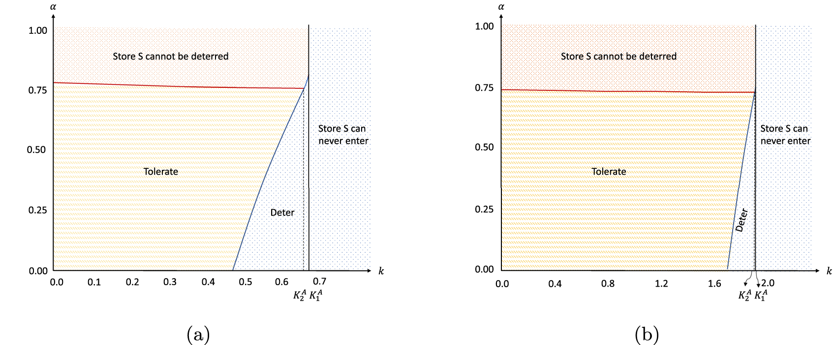
Store R’s equilibrium deterrence strategy against a type (B) store S. Setting: $c_s=0.7$ , (a) store R’s deterrence strategy against a type (B) store S with ${\beta }^B({\gamma }^B)=1+3\cdot {\gamma }^B$ and, (b) store R’s deterrence strategy against a type (B) store S with ${\beta }^B({\gamma }^B)=1+8\cdot {\gamma }^B$ .

First, recall from Proposition 2 and 4 that the optimal deterrence strategy of store R against store S depends on both store S’s entry cost $k$ and store R’s cost advantage $\alpha$ . Observe that Figures 6 and 7 resemble Figure 3, indicating that the optimal deterrence strategies of store R against store S for the case when the donating proportion $\gamma$ is endogenously determined by store S, possess a similar structure as stated in Propositions 2 and 4 for the base model when $\gamma$ is exogenously given.

Next, observe from Figure 6 that, as the warm-glow factor for a type (A) store S, denoted as $b^A$ , increases from $3$ (Figure 6(a)) to $8$ (Figure 6(b)), consumers can derive more utility by shopping at a type (A) store S, making it difficult for store R to deter. For this reason, store R is more likely to tolerate its entry. This is evident as the yellow “tolerance” region becomes larger in Figure 6(b). This line of logic continues to hold for a type (B) store S. Specifically, when the warm-glow factor for a type (B) store S, denoted as $b^B$ , increases from $3$ (Figure 7(a)) to $8$ (Figure 7(b)), it becomes easier for a type (B) store S to enter the market. This can be seen from the larger yellow “tolerance” region in Figure 7(b) compared to Figure 7(a).

Finally, observe from Figure 6(a) and Figure 7(b) that, when the warm-glow factor $8=b^B>b^A=3$ (so that a type (B) store S can generate a stronger warm-glow effect), it can be seen that the sizes of both the yellow and the pink regions (i.e., regions within which a store S can enter) are larger in Figure 6(a) than in Figure 7(b). However, the size of the “deterrence” region, along with the region where store S can never enter the market (colored in blue), is smaller in Figure 6(a). It reveals that it is more likely for a type (A) store S to enter the market than a type (B) store S even when a type (B) store may generate a stronger warm-glow effect.

Remark 1

In the case when the donating proportion is endogenously determined by each type of store S, the incumbent store R’s optimal deterrence strategy against store S yields the same structural results as when the donation proportion is exogenously given. Moreover, as the warm-glow factor increases, the incumbent store R becomes less aggressive in deterring store S. Additionally, the incumbent store R is generally more likely to deter a type (B) store S (that donates revenue) rather than a type (A) store S (that donates profit) unless a type (B) store S can generate a significantly stronger warm-glow effect than a type (A) store S.

7.2. Equilibrium Results Analysis

Next, we shall numerically analyze how the parameters would affect the optimal ${\gamma }^j,j\in \{A,B\}$ set by two types of store S along with other corresponding equilibrium outcomes.

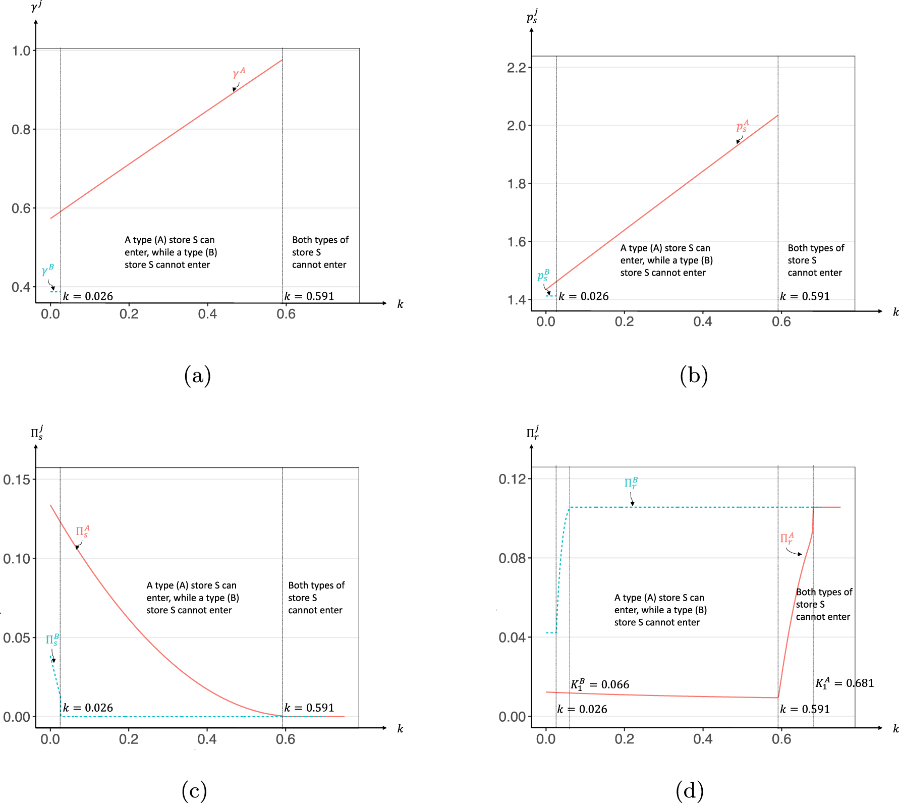
7.2.1. Impact of Store S’s Entry Cost $k$ on the Equilibrium Results

First, we examine the impact of store S’s entry cost $k$ by setting $c_s=0.7$ , $\alpha =0.5$ , and $b^A=b^B=3$ . Observe from Figure 8(a) that a type (A) store S can enter the market more easily (when $k<0.591$ ) than a type (B) store S (who can only enter when $k<0.026$ ). Also, observe from Figure 8(a) and (b) that, when store S can enter the market, as the entry cost $k$ increases, a type (A) store S will increase its optimal donating proportion ${\gamma }^A$ to boost consumer utility and increase its price $p_s^A$ to offset the higher entry cost $k$ . Interestingly, this behavior is not present for a type (B) store S. Specifically, the optimal ${\gamma }^B$ and $p_s^B$ set by a type (B) store S remain unchanged regardless of $k$ . This is because a type (A) store S deducts its entry cost $k$ from its profit before donating, whereas a type (B) store S donates a portion of its revenue, which is independent of $k$ .

Figure 8.

Equilibrium results when $k$ varies. Setting: $c_s=0.7$ , $\alpha =0.5$ , ${\beta }^j({\gamma }^j)=1+3\cdot {\gamma }^j$ with $j\in \{A,B\}$ , (a) optimal ${\gamma }^j$ set by store S when $k$ varies, (b) optimal $p_s^j$ set by store S when $k$ varies, (c) ${\mathrm{\Pi }}_s^j$ in equilibrium when $k$ varies, and (d) ${\mathrm{\Pi }}_r^j$ in equilibrium when $k$ varies.

Figure 8(c) and (d) depict the corresponding profits of store S and store R, respectively. It is intuitive that both types of store S’s optimal profit will decrease when its entry cost $k$ increases. However, the impact of $k$ on the incumbent store R’s profit is more nuanced. First, let us examine store R’s profit in the face of the entry threat from a type (A) store S. Interestingly, when $k<0.591$ so that store R chooses to tolerate the entry of a type (A) store S, store R’s profit (in red) decreases slightly in $k$ . This is because as $k$ increases, a type (A) store S also increases its donating proportion ${\gamma }^A$ , thus by tolerating its entry, store R needs to lower its price further to recapture market share, thereby squeezing its profit. However, when $0.591<k<K_1^A=0.681$ store R chooses to deter a type (A) store’s entry, which will boost store R’s profit as $k$ increases. This is because a higher entry cost makes it easier for store R to deter store S. Finally, when $k>K_1^A=0.681$ store S can never enter the market, store R’s profit remains unaffected by $k$ . Next, in the face of the potential entry of a type (B) store S, when store R chooses to tolerate its entry when $k<0.026$ , store R’s optimal profit will not be affected by the entry cost $k$ . This is because a type (B) store S’s optimal ${\gamma }^B$ and $p_s^B$ both remain unchanged when $k$ as shown in Figure 8(a) and (b). Also, similarly to a type (A) store S, when $0.026<k<K_1^B=0.066,$ store R chooses to deter the entry of a type (B) store S, store R’s profit increases with the entry cost $k$ . When $k>K_1^B=0.066,$ store S can never enter the market, store R’s profit will remain unchanged.

Figure 8 also indicates that when $b^A=b^B$ , upon entry, a type (A) store S set a higher donating proportion ${\gamma }^A$ along with a higher price $p_s^A$ compared to a type (B) store S (as shown in Figure 8(a) and (b)). Additionally, upon entry, a type (A) store S attains a higher profit ${\mathrm{\Pi }}_s^A$ (Figure 8(c)), resulting in a more significant squeeze on store R’s profit (Figure 8(d)).

7.2.2. Impact of Store R’s Cost Advantage $\alpha$ on the Equilibrium Results

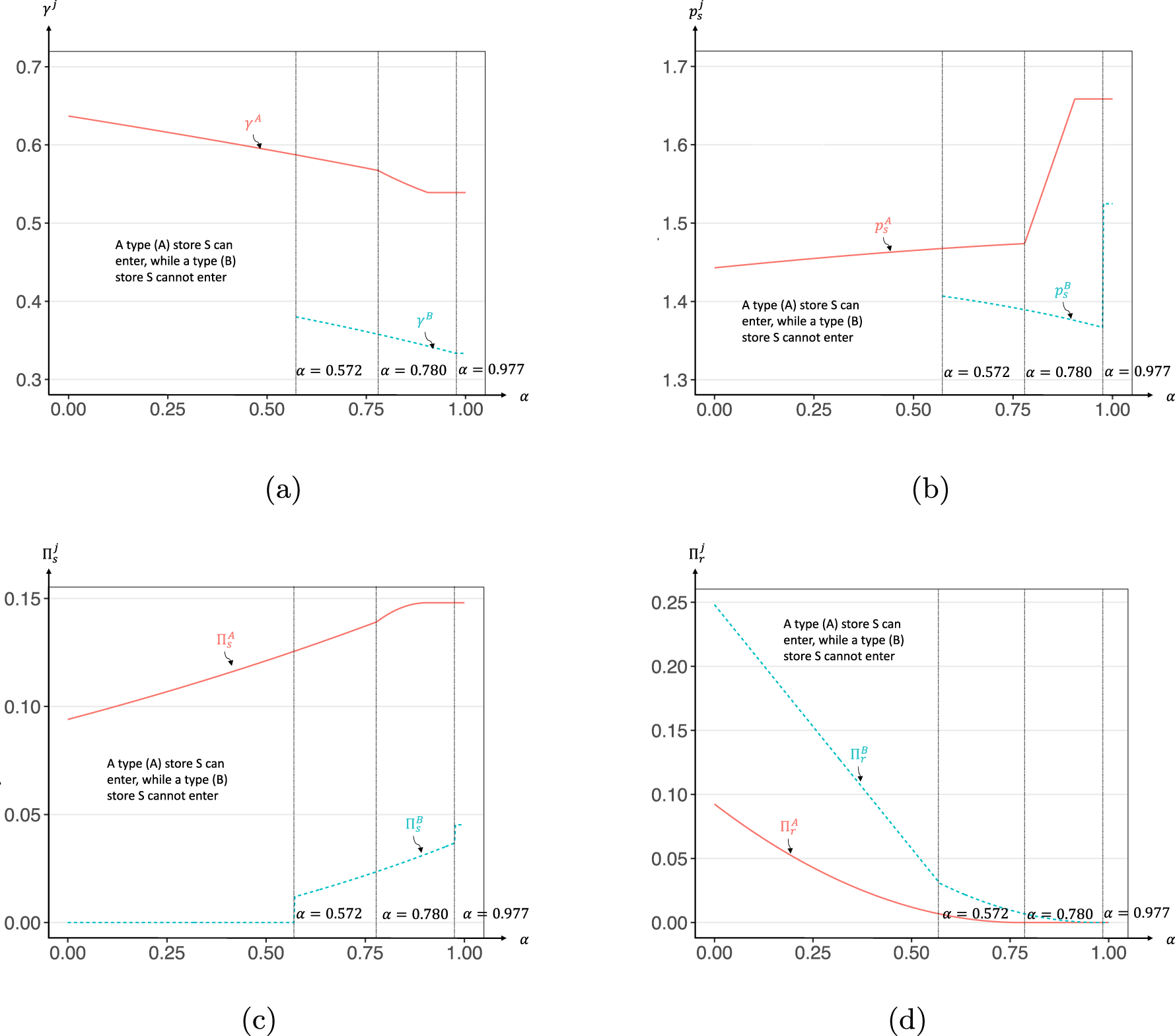
Next, we numerically examine the impact of store R’s cost advantage $\alpha \equiv \frac{c_r}{c_s}<1$ on the equilibrium results for the case when $\gamma$ is endogenously determined by store S. We set $c_s=0.7$ , $k=0.03$ and $b^A=b^B=3$ . Recall that $\alpha \equiv (c_r/c_s)$ so that as $\alpha$ increases, store R’s cost advantage over store S is lower. Observe from Figure 6(a) and 7(a) that when $k=0.03$ , a type (A) store S can always enter the market, while whether a type (B) store S can enter or not depends on $\alpha$ . Observe from Figure 9(a) that, when $\alpha >0.572$ , a type (B) store S can enter the market. Moreover, Figures 6(a) and 7(a) also show that when $\alpha$ is very large so that store R’s cost advantage is low, not only can store S enter the market, but it can also drive store R out of the market. This is also supported by Figure 9(d) that when $\alpha >0.780$ , store R’s profit becomes $0$ upon a type (A) store S’s entry; and when $\alpha >0.977$ , store R will be squeezed out upon a type (B) store S’s entry.

Figure 9.

Equilibrium results when $\alpha$ varies. Setting: $c_s=0.7$ , $k=0.03$ , ${\beta }^j({\gamma }^j)=1+3\cdot {\gamma }^j$ with $j\in \{A,B\}$ : (a) optimal ${\gamma }^j$ set by store S when $\alpha$ varies, (b) optimal $p_s^j$ set by store S when $\alpha$ varies, (c) ${\mathrm{\Pi }}_s^j$ in equilibrium when $\alpha$ varies, and (d) ${\mathrm{\Pi }}_r^j$ in equilibrium when $\alpha$ varies.

Observe from Figure 9(a) that, upon entry, both types of store S will reduce their donating proportion ${\gamma }^j$ as $\alpha$ increases. This is due to the fact that store S can enter the market even with a lower warm-glow effect when store R’s cost advantage is sufficiently low (i.e., when $\alpha$ is high). Therefore, as $\alpha$ increases, both types of store S can afford to lower their optimal donating proportion in order to maximize their profit. Additionally, when store R’s cost advantage decreases (i.e., $\alpha$ increases), a type (A) store S can also afford to charge a higher price, whereas a type (B) store S will lower its price upon entry. Hence, the change in store S’s optimal price $p_s^j$ with respect to $\alpha$ (whether increasing or decreasing) is type-specific. Finally, we observe from Figure 9(c) that the optimal profits of both types of store S increase with $\alpha$ . Consequently, store R’s profit decreases as $\alpha$ increases due to lower cost advantage (Figure 9(d)).

7.2.3. Impact of Relative warm-glow Factor $\frac{b^B}{b^A}$ on the Equilibrium Results

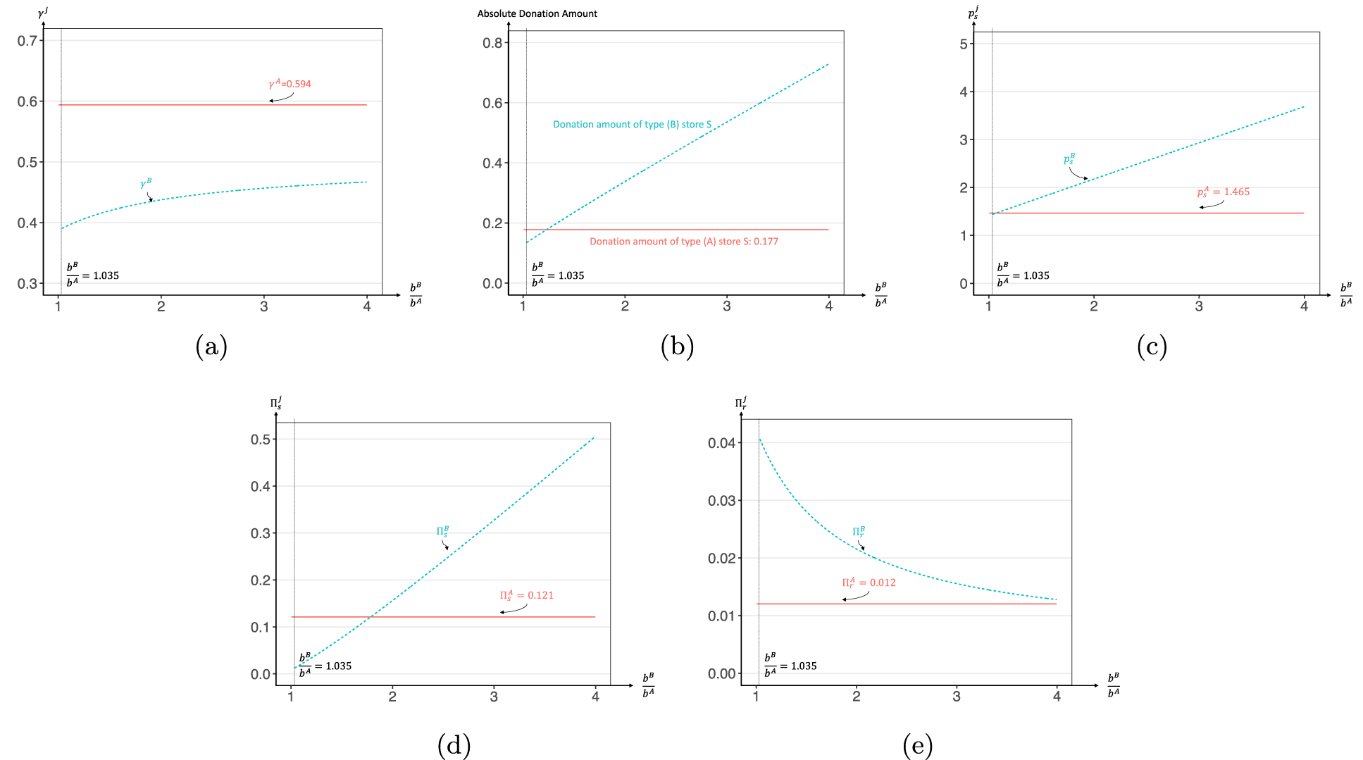
We now examine the case where the warm-glow factors $b^A$ and $b^B$ are store “type-specific.” As before, we set $c_s=0.7$ , $k=0.03$ , $\alpha =0.5$ , and fix $b^A=3$ so that ${\beta }^A({\gamma }^A)=1+3\cdot {\gamma }^A$ . In this case, store R chooses to tolerate a type (A) store S’s entry, which can be observed from Figure 6(a). Here, we vary $b^B$ so that the corresponding ratio $b^B/b^A$ can vary between $1$ and $4$ . In doing so, we can examine the impact of the warm-glow factor ratio $b^B/b^A$ on the equilibrium results. Observe from Figure 10 that, only when $(b^B/b^A)>1.035$ can a type (B) store S enter the market.

Figure 10.

Equilibrium results when $b^B$ ( $\frac{b^B}{b^A}$ ) varies. Setting: $c_s=0.7$ , $k=0.03$ , $\alpha =0.5$ , $b^A=3$ so that ${\beta }^A(\gamma )=1+3\cdot \gamma$ , (a) optimal donation proportion ${\gamma }^j$ when $b^B$ ( $b^B/b^A$ ) varies, (b) Optimal absolute donation amount when $b^B$ ( $b^B/b^A$ ) varies], (c) Optimal $p_s^j$ when $b^B$ ( $b^B*b^A$ ) varies], (d) ${\mathrm{\Pi }}_s^j$ in equilibrium when $b^B$ ( $b^B/b^A$ ) varies], and (e) ${\mathrm{\Pi }}_r^j$ in equilibrium when $b^B$ ( $b^B/b^A$ ) varies].

From Figure 10(a), observe that the optimal ${\gamma }^B$ set by a type (B) store S increases with the warm-glow factor $b^B$ (i.e., as $(b^B/b^A)=(b^B/3)$ increases). Interestingly, even when the ratio $b^B/b^A$ becomes very high so that $b^B$ is much higher than $b^A=3$ , the optimal ${\gamma }^B$ remains lower than the optimal ${\gamma }^A$ . This finding suggests that, as the warm-glow factor $b^B$ increases, although a type (B) store S will increase its donation proportion, it still cannot afford to set ${\gamma }^B$ as large as ${\gamma }^A$ because the donation is based on revenue and its profitability needs to be ensured. This observation is consistent with practical implications. However, upon examining the absolute donation amount, Figure 10(b) suggests that either a type (A) or a type (B) store S would donate a greater amount. Next, it can be observed from Figure 10(c) that the optimal $p_s^B$ also increases with the warm-glow factor $b^B$ . Furthermore, as $b^B$ increases, a type (B) store S would charge a higher $p_s^B$ compared to $p_s^A$ in order to ensure profitability. Figure 10(d) shows that when the warm-glow factor $b^B$ increases, a type (B) store can also earn a higher profit, which can be even higher than a type (A) store’s profit. Nevertheless, it is worth noting that, even when $b^B>b^A$ , a type (B) store S may still get a lower profit than a type (A) store S unless it can generate a much stronger warm-glow effect than a type (A) store S. Figure 10(e) presents the profit of the incumbent store R, which decreases with $b^B$ .

8. Conclusion

In recent years, there has been a strong shift in consumer preferences toward social responsibility, and this shift creates a suitable environment for new socially responsible retailers to enter the market. This observation motivated us to study entry conditions of a commonly observed class of socially responsible retailers that pre-commit to donating a certain proportion of their profits (type (A)) or revenues (type (B)). Our equilibrium analysis revealed that the incumbent retailer’s deterrence strategy depends on its cost advantage (captured by $\alpha$ ) and the social retailer’s entry cost (captured by $k$ ). An interesting finding is that even when the incumbent retailer has the power to deter the entry of the social retailer, it may still choose to tolerate its entry. We also compare the two types of social retailers. We find that a type (A) social retailer poses a higher entry threat for the incumbent than type (B) social retailer, yet interestingly, the incumbent is more aggressive in deterring the entry of type (B) social retailer. Thus, it is easier for a type (A) social retailer to enter the market unless a type (B) social retailer can generate a sufficiently higher warm-glow effect than a type (A) store. This managerial insight may guide entrepreneurs who aim to establish social retailers to pre-commit to donate a certain proportion of their profits rather than revenues.

Our paper is the first attempt to understand the market dynamics between an incumbent for-profit retailer and a common class of socially responsible retailers. There are several avenues for further research. For instance, we have examined a common class of social retailers, but it is of interest to compare very different classes of social retailers (e.g., one type donates one unit to charity when a consumer buys one unit, and the other type donates the revenue to charity). Also, there are other classes of social retailers such as food cooperatives. Studying the entry of such cooperatives would be an interesting research avenue to pursue.

Supplemental Material

sj-pdf-1-pao-10.1177_10591478231224935 - Supplemental material for Should an Incumbent Store Deter Entry of a Socially Responsible Retailer?

Supplemental material, sj-pdf-1-pao-10.1177_10591478231224935 for Should an Incumbent Store Deter Entry of a Socially Responsible Retailer? by C Gizem Korpeoglu, Ersin Körpeoğlu, Christopher S Tang and Jiayi Joey Yu in Production and Operations Management