
Abstract
This article studies an appointment scheduling problem where a service provider dynamically receives appointment requests from a random number of customers. By leveraging the randomness of the number of potential customers, we develop a nonsequential appointment scheduling policy as an alternative to the conventional first-come-first-served (FCFS) policy. This allows for more flexibility in managing appointment scheduling. To calculate the optimal policy, we develop a branch-and-bound algorithm in which the lower bound is estimated using multiple approaches, such as optimality conditions, dynamic programming for calculating FCFS policy, and the shortest path reformulation. Through numerical studies, we observe that nonsequential appointment scheduling is particularly advantageous in systems characterized by highly fluctuating customer numbers or low congestion. In such cases, leaving gaps between appointments for potential future arrivals proves to be a more appropriate strategy. We also evaluate the performance of heuristics proposed in prior literature and provide insights into situations where these heuristics can be effectively applied.
Introduction
Background
Appointment scheduling plays a vital role in achieving operational excellence within a service system by minimizing customer waiting time and maximizing the utilization of system resources. In practice, appointment scheduling can be carried out through various approaches, including offline and online scheduling and inter and intraday scheduling.
In offline appointment scheduling, the system provides appointment schedules after all requests have arrived, whereas, in online appointment scheduling, the system offers an appointment upon receiving a customer’s request, regardless of the exact number of upcoming customers (Ahmadi-Javid et al., 2017). In interday scheduling, the system aims to assign appointment requests to future days, taking into account customer preferences and indirect waiting costs (the time between the appointment request date and the appointment date provided) (Gupta and Wang, 2008; Keyvanshokooh et al., 2021; Liu et al., 2019). In intraday scheduling, the system schedules specific service start times for customers with predetermined appointment dates, aiming to strike a balance between waiting times, idle times, and overtime within a single day’s operation (Chen and Robinson, 2014; Erdogan et al., 2015).
This article investigates an online intraday appointment scheduling problem with a random number of customers. Such problems commonly arise in healthcare systems, particularly when certain doctors are only available for duty on specific days of the week, as illustrated, for example, by the timetable of specialists of a hospital in Hong Kong. 1 While our research primarily focuses on intraday scheduling, it is also relevant to interday scheduling. In certain interday appointment scheduling systems, customers are initially granted the opportunity to select an available service day, after which the system assigns them a specific start time for their appointment. This is illustrated by the appointment system of MaxHealth, 2 where customers are given the option to choose between morning, lunchtime, or afternoon medical appointments on a particular day. Since customers call in dynamically, the number of upcoming customers on an arbitrary day fluctuates.
Major Issues
The general difficulty of the online intraday appointment scheduling problem stems from the uncertainty of the number of customers, which leads to the sequencing issue of the customers. In certain systems, customers are scheduled on a first-come-first-served (FCFS) basis, where those submitting requests earlier will be assigned earlier service start times. We refer to such a process as sequential appointment scheduling. An example of such a system can be observed in HA Go, 3 an APP used by the Hong Kong public hospital system to provide various services to patients. One particular function of the app is to manage appointments. Once a patient selects a clinic and submits an appointment request, the patient will be provided with the earliest available slot. In some other systems, nonsequential appointment scheduling is adopted in which customers submitting requests early may be given later service start times. To illustrate this disparity, we provide Example 1, depicted in Figure 1, to highlight the distinction between sequential and nonsequential appointment scheduling.
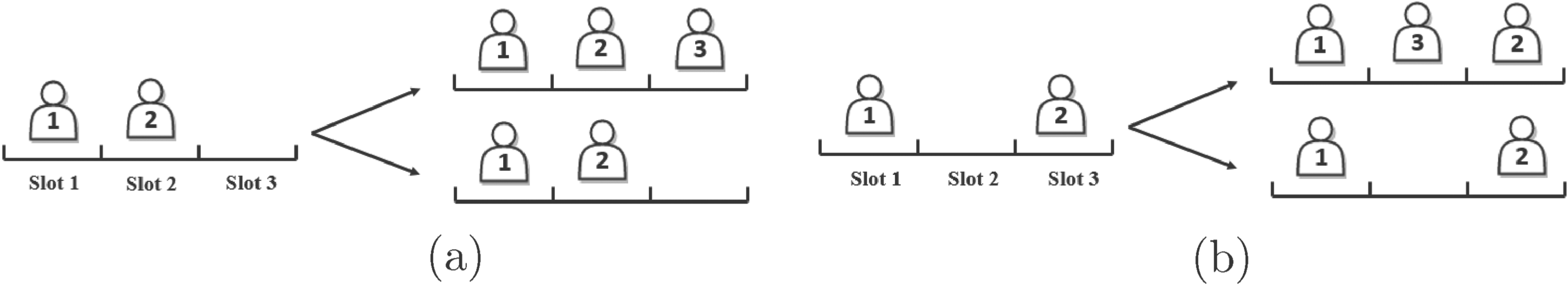
Sequential scheduling and nonsequential scheduling for Example 1: (a) sequential scheduling; (b) nonsequential scheduling.
Consider a single server with a service horizon equally divided into three time slots. Each slot can be offered to only one customer. There are two or three potential customers whose service times are identically and independently distributed, and the mean of the service times is equal to the length of a time slot.
In sequential appointment scheduling, time slot
In nonsequential scheduling, one possible scheduling principle is to assign slot 3 to the second customer submitting the request, thereby reserving slot 2 for the potential request from a third customer. This strategy leads to two possible final appointment schedules, as shown in Figure 1(b). By comparing the overall expected waiting times for customers in Figure 1(a) and (b), we can see that the second customer in Figure 1(b) experiences a much shorter waiting time when there are only two customers. This is because, in this case, the empty slot 2 absorbs the impact of the first customer’s randomly varying service time. Although this alone may not be sufficient to firmly conclude that schedule (b) is superior to schedule (a), as other factors such as system idle costs and overtime costs also need consideration, it does highlight the potential advantages of nonsequential scheduling when dealing with an uncertain number of customers.
Such an online intraday nonsequential appointment scheduling problem has been studied in the literature (Chen and Robinson, 2014; Erdogan et al., 2015). These studies reveal the potential benefits of considering sequencing issues when dealing with a random number of customers. However, their focus primarily revolves around proposing heuristics. There is still no algorithm for determining the optimal schedule.
In practice, in addition to uncertainty regarding the number of customers, the task of determining optimal appointments is further complicated by uncertainties in customer behavior. In many appointment service systems, cancellations, late arrivals, and no-shows occur frequently. These behaviors disrupt schedules and increase system idle time (Kong et al., 2020; Liu et al., 2010; Pan et al., 2021). While research has examined the influence of these behaviors on optimal schedules, a comprehensive investigation of these factors in online appointment scheduling problems is lacking.
Our work simultaneously considers three potential customer behavior cases, namely last-minute cancellations, late arrivals, and no-shows. First, if a customer cancels their appointment and notifies the system prior to the scheduled appointment time, the system can bypass them and proceed to serve the next customer. Consequently, there is no waiting time cost incurred for these customers who cancel at the last minute. This is referred to as a last-minute cancellation (Liu et al., 2010). Second, in the event of a customer arriving late without prior notification, the system will wait for the customer instead of serving the next customer. The duration of the customer’s lateness will not be counted as part of their waiting time. This is referred to as a late arrival (Samorani and Ganguly, 2016). Third, the system cannot confirm whether a customer is a no-show until
We summarize the main results and contributions of our work from three perspectives, namely, the positioning of our model, the algorithms for problem-solving, and the managerial insights for operational guidelines.
For modeling, we first study a basic online appointment scheduling problem with a stochastic number of customers. This particular problem was previously explored by Chen and Robinson (2014) and Erdogan et al. (2015). These studies primarily tackled cases involving continuous appointment times and proposed heuristic approaches for determining appointment sequences. In contrast, our work addresses the discrete appointment times scenario and is the first to optimally solve the online appointment scheduling problem. Significantly, our model can be expanded to incorporate last-minute cancellations, late arrivals, and no-shows by customers, thereby introducing additional complexities to the online scheduling problem beyond the scope of Chen and Robinson (2014) and Erdogan et al. (2015).
With regard to problem-solving, we develop a novel branch-and-bound (B&B) algorithm that integrates two perspectives for this particular problem. First, our problem can be perceived as a dynamic assignment problem, in which the decision is an appointment scheduling principle that specifies the time slot assigned to each customer upon request. Second, our problem can also be formulated as a shortest path problem on a layered directed network, in which each vertex corresponds to a possible state (a term that is formally defined below). Consequently, an appointment scheduling principle can be modeled by the path from a specified source to a specified sink, with the shortest path providing the optimal solution. Both perspectives possess inherent advantages and some disadvantages. To mitigate these drawbacks, we explore various properties of these two models and subsequently develop a set of rules specifically designed to speed up the search process for optimal policies. Hence, the distinctiveness of our algorithm lies in its ability to leverage the strengths of both perspectives while circumventing their respective limitations.
Numerical studies have also yielded several managerial insights, which are presented as follows:
In scenarios where the number of customers fluctuates significantly or the system is not heavily congested, it is advisable to adopt nonsequential appointment scheduling, that is, leaving some time slots open in between for future arrivals. Patient lateness will substantially increase system costs, whereas cancellations and no-shows can partially offset system costs for that particular day. For an optimal online policy, we can always find an implemented online policy that is close to or even identical to the corresponding optimal offline policy. The point at which this correspondence appears is closely related to factors such as the expected number of customers, the customer number with the highest probability, and the maximum weighted offline cost. This correspondence pattern motivates us to utilize several offline optimal policies as approximations for an online policy. Regarding the heuristics, we compare two approaches: a pairwise interchange proposed in the literature and a greedy algorithm proposed in this study. Our comparison reveals that the pairwise interchange performs better in congested systems. Conversely, the greedy algorithm demonstrates good performance within relatively idle systems. The combination of the two heuristics results in a well-performing heuristic that is suitable for general service systems.
The remainder of this article is organized as follows. In Section 2, we review the relevant literature. In Section 3, we describe the problem, derive optimal properties, and extend our model. In Section 4, we investigate special cases of the sequential scheduling principle. In Section 5, we develop a B&B algorithm. In Section 6, we present the computational results. We conclude this article in Section 7. The proofs of all theorems are available in the E-Companion of the Supplemental Material.
Appointment scheduling problems have been investigated in many service industries. Most studies are driven by healthcare management (Deng et al., 2019; Zacharias and Yunes, 2020; Bandi and Gupta, 2020), and some studies contribute to general service systems (Mancilla and Storer, 2012; Kemper et al., 2014; Mak et al., 2014b; Qi, 2017). For comprehensive reviews, refer to Cayirli and Veral (2003), Gupta and Denton (2008), Ahmadi-Javid et al. (2017), and Youn et al. (2022). To keep the review concise, we concentrate on two streams of literature, one on nonsequential appointment scheduling and the other on cancellations, late arrivals, and no-shows.
In offline appointment scheduling, several studies investigate the relationship between the optimal sequence and the distribution of service time. They propose certain heuristic rules, such as the smallest-variance-first rule, which prove to be optimal under some conditions (Weiss, 1990; Wang, 1999; Denton et al., 2007; Mak et al., 2014a; Kemper et al., 2014; Kong et al., 2016; Guda et al., 2016; de Kemp et al., 2021). Moreover, the impact of various customer attributes on the optimal sequencing decision has been explored, such as customers with different probabilities of being a no-show (LaGanga and Lawrence, 2012; Zacharias and Pinedo, 2014) and different delay-unpleasantness measures (Qi, 2017).
In online appointment scheduling, most studies in this stream of the literature are centered around healthcare applications, where customers are classified into two types, that is, routine customers and same-day (or walk-in) customers. Routine customers are scheduled with sufficient prior information, whereas same-day customers and walk-in customers introduce a source of uncertainty into the system. Throughout the existing literature, the treatment of same-day and walk-in customers differs markedly.
Same-day customers must submit an appointment request before the start of the working horizon in order to receive service. Our work is closely related to such problems, which were initially explored by Chen and Robinson (2014) and Erdogan et al. (2015). Chen and Robinson (2014) considered sequencing and scheduling appointments for both homogeneous routine patients and heterogeneous same-day patients. The critical difference between our work and theirs is that Chen and Robinson (2014) employed heuristic rules to identify appointment sequences, whereas we design an algorithm to determine the optimal sequence. Furthermore, Chen and Robinson (2014) assumed that a doctor’s day ends once he or she finishes attending to the last scheduled patient. They acknowledge that their heuristic structure ceases to be applicable if the doctor is obligated to remain until the end of the working horizon. This particular scenario is the focus of our investigation. Erdogan et al. (2015) delved into the same model and develop a stochastic program. They also design heuristic sequencing rules to solve this problem. What distinguishes our work from Erdogan et al. (2015) is that they enumerate appointment sequences using an integer program, whereas we implicitly enumerate them using a B&B strategy. Another technical difference is that Chen and Robinson (2014) and Erdogan et al. (2015) assumed that appointment times are continuous, for which a mathematical program is a natural solution tool. In contrast, we consider appointment times to be discrete (e.g., multiples of 10 min), a more practical approach, and subsequently employ a tailored B&B algorithm.
Distinct from same-day customers, walk-in customers arrive unpredictably during the service horizon and have the opportunity to receive service without a prior appointment. Green et al. (2006) established dynamic priority rules for admitting customers to service, particularly when two types of customers are waiting simultaneously. Freeman et al. (2016) examined the scheduling of routine customers, emphasizing the need to serve potential walk-in customers within a specified waiting time upon arrival. Zacharias and Yunes (2020) studied an online scheduling problem, in which general stochastic service times, no-shows, nonpunctuality, and walk-ins are jointly considered. They investigate the multi-modularity of the objective function in a general setting. Wang et al. (2020) studied a similar problem to that of Zacharias and Yunes (2020) but from a fundamentally different angle, reformulating the challenging problem to a tractable mathematical program.
In addition, online appointment scheduling problems can also be categorized into intraday (i.e., at what time) and interday (i.e., on which day) scheduling. Most of the above online scheduling literature focuses on intraday scheduling. In interday appointment scheduling, there exists a concept analogous to nonsequential scheduling known as the “leaving holes” strategy (Patrick et al., 2008; Sauré and Puterman, 2014; Izady, 2019). This strategy involves reserving some capacity to accommodate potential same-day demand while allocating daily capacity for advance booking demand. Patrick et al. (2008) explored this strategy in the context of scheduling surgical patients with varying priorities. Truong (2015) characterizes an optimal policy for the dynamic interday problem and derives an efficient algorithm for policy computation. Wang and Truong (2018) investigated a multi-priority interday scheduling problem that incorporates cancellations, with the competition ratio serving as the optimization criterion. Wang et al. (2019) considered sequential appointment scheduling in a network of stations with exponential service times, no-shows, and overbooking. Keyvanshokooh et al. (2021) studied an online resource allocation problem in which arrivals with different service times and rewards make appointments on several servers. Keyvanshokooh et al. (2022) addressed healthcare coordination aimed at setting appointments for pairs of sequential visits and minimizing the indirect access time. Zacharias et al. (2022) simultaneously considered both inter and intraday scheduling in dynamic scheduling decisions.
In addition to offline and online scheduling problems, there is another category of appointment scheduling problem known as “myopic scheduling.” In myopic scheduling, the system immediately schedules an appointment as soon as a customer submits a request, without considering potential future requests (Muthuraman and Lawley, 2008; Zacharias and Pinedo, 2014). The key distinction between myopic and online scheduling lies in their consideration of future requests, with online scheduling taking into account such possibilities while myopic scheduling does not.
The second body of literature pertains to the challenges posed by last-minute cancellations, late arrivals, and no-shows. Past research has made significant contributions to appointment scheduling with no-shows and minimizing their impact on schedules, thus achieving a better balance between demand and capacity. Some studies have focused on homogeneous no-show probabilities (Green et al., 2006; Hassin and Mendel, 2008), and others have delved into heterogeneous no-show rates (Zeng et al., 2010; Chen and Robinson, 2014) and time-dependent no-show rates (Kong et al., 2020; Wang et al., 2020; Zacharias and Yunes, 2020). Additionally, some papers consider the rescheduling of a no-show or canceled appointment within the context of interday scheduling problems (Xie et al., 2021). However, relatively few papers have focused on cancellations (Liu et al., 2010) and late arrivals (Deceuninck et al., 2018; Pan et al., 2021).
It is worth mentioning that the existing literature presents various definitions of cancellations and no-shows. In the study by Liu et al. (2010), the focus is on interday cancellations, where customers can cancel their appointments prior to the scheduled day and the vacant slots resulting from these cancellations can be allocated to future customers. In addition, Chen and Robinson (2014) assumed that if a patient fails to arrive promptly for their appointment, the system can immediately recognize the customer as a no-show, skip them, and serve the next customer, which is equivalent to a last-minute cancellation in our work. Regarding no-shows, according to Zacharias and Yunes (2020), the system does not need to wait for a specific patient at their appointment time. Instead, the system continues to serve customers who have already arrived and are waiting in the queue. Consequently, the actual order of service may differ from the scheduled sequence. In the study of Xie et al. (2021), cancellations and no-shows are considered synonymous and referred to as “missed appointments.” Some papers consider two features simultaneously, including both no-shows and late arrivals (Zacharias and Yunes, 2020; Jiang et al., 2019; Pan et al., 2021; Jouini et al., 2022), as well as the combination of no-shows and cancellations (Liu et al., 2010; Feldman et al., 2014; Diamant, 2021). However, there are limited studies that comprehensively address the triad of last-minute customer cancellations, late arrivals, and no-shows in the context of online appointment scheduling. Furthermore, Zacharias and Yunes (2020) shed light on the exponential complexity of objective function evaluations when nonpunctual patients are taken into account. To the best of our knowledge, the simultaneous consideration of last-minute customer cancellations, late arrivals, and no-shows in online appointment scheduling is novel in the existing literature.
Model and Properties
Problem Description and Dynamic Assignment Model
To enhance comprehension of the model, we initially present the problem formulation without incorporating last-minute cancellations, late arrivals, or no-shows. Subsequently, in Section 3.4, we extend this model to encompass the simultaneous consideration of these three stochastic features.
We consider a scenario where there is a single server attending to a random number of customers. The server is available for a specified time interval, denoted as The assigned time slots and corresponding service start times for Example 2.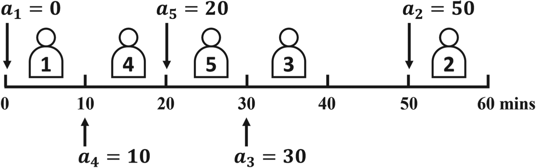
The service horizon is divided into
In the online appointment scheduling problem, the decision can be represented by an appointment policy, formally defined as follows.
An appointment policy is represented by a vector
A system has
Henceforth, for clarity and to distinguish between various policies, we employ additional boldface Greek letters, such as
As the number of customers
For a policy
The evaluation of a policy
For a partial policy
The state vector
Consider two appointment policies
Given a partial policy
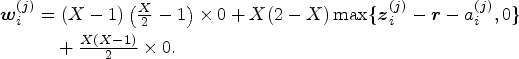
First, we model the waiting time of a customer. Similar to the definition of 
Finally, we consider the system overtime cost, which can be represented by the waiting time of a dummy customer who is the first to call and is scheduled to start service at time
Then, the state cost of 
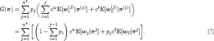
Overall, the objective function 
When the number of customers is
Thus, the objective function 

When the total cost per unit of idle time plus per unit of overtime
We introduce two properties of optimal appointment policies that outline the circumstances in which a specific partial policy does not result in an optimal policy.
The first property focuses on the state costs of two partial policies derived from a common partial policy. We refer to it as the property on state cost.
(Property on State Cost)
Given a partial policy
Theorem 1 indicates that when scheduling the
Second, we study partial policies from the aspect of the marginal state cost. For this purpose, we introduce the concept of the expected marginal cost brought by the
(Property on Marginal State Cost)
Given a partial policy
Theorem 2 shows that the new state cost should not be relatively too low; otherwise, the corresponding new partial policy cannot be optimal. It establishes a minimum threshold for the marginal cost when scheduling an additional customer. Moreover, Theorem 2 implies that, in an optimal appointment policy, the marginal cost should increase with
(Increasing Marginal State Cost)
There exists an optimal appointment policy
In Section 5, based on Theorems 1 and 2, and Corollary 1, we propose a set of elimination rules and establish a lower bound to speed up the search process within our B&B algorithm.
Shortest Path Model
Our appointment scheduling problem can also be modeled as a shortest path problem on a directed network with
To represent a partial policy
A shortest path network with Shortest path model of the scheduling problem with 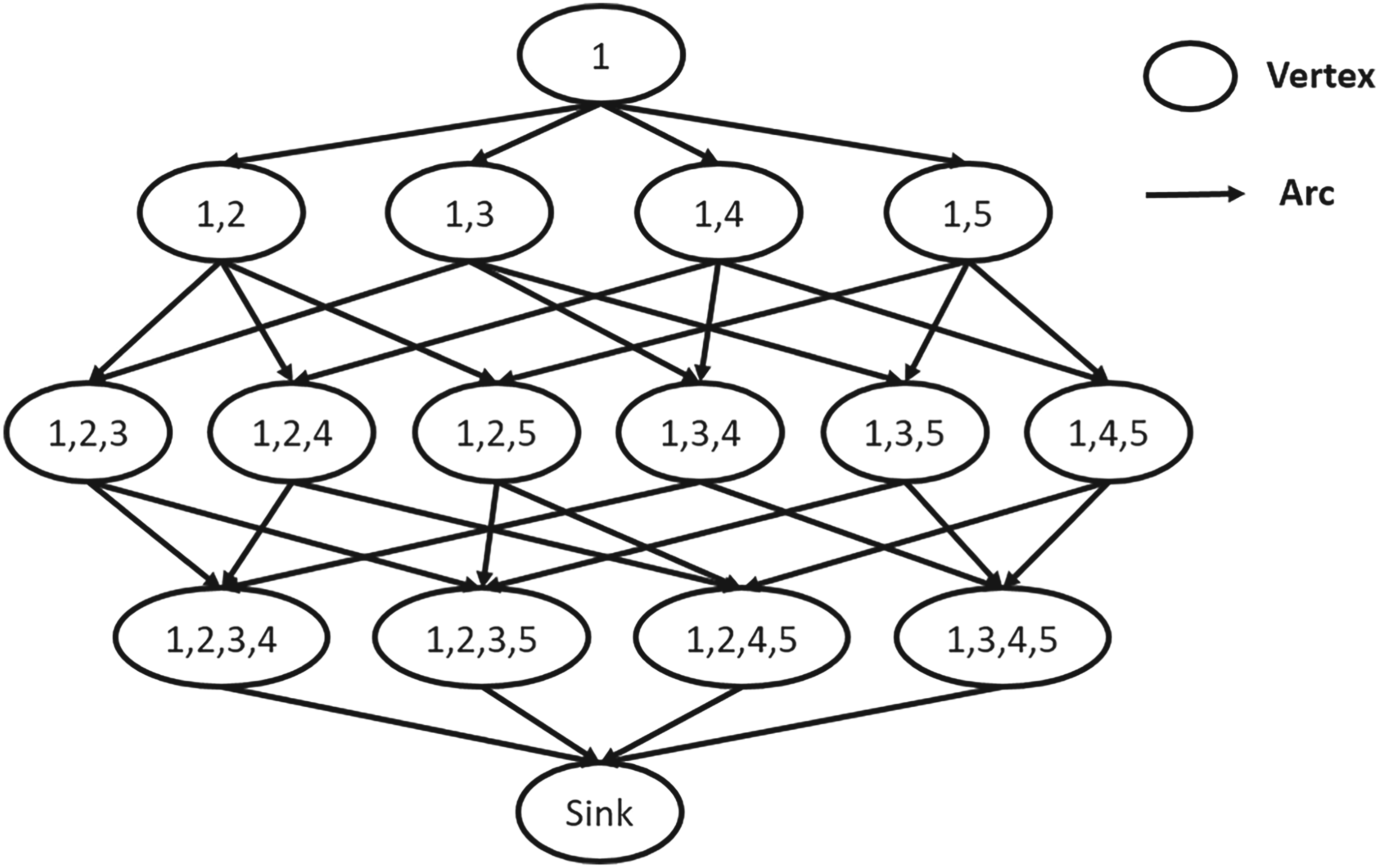
In problems with a general scale, the constructed network exhibits an exponential size, where the number of vertices is in
Given two subpaths
Note that Theorem 1 is a special case of Theorem 3. Both theorems serve as valuable tools for evaluating the optimality of partial policies. Theorem 1 specifically focuses on the comparison between two partial policies derived from a shared partial policy. Theorem 3 is applicable to a larger set of partial policies. It is worth mentioning that Theorem 3 requires additional computational effort, as it entails the calculation of the path cost.
Besides the new optimal condition, this shortest path model will contribute further to our B&B algorithm, which is discussed in Section EC.1 of the Supplemental Material.
Last-Minute Cancellations, Late Arrivals, and No-Shows
Up to now, we assume that all customers will arrive at the system punctually. In this section, we extend the scope of our model by incorporating all three random features into our online appointment scheduling problem.
Prior to the scheduled appointment, there is a probability that a customer may cancel their appointment and notify the system, denoted as
Subsequently, we denote the status of all potential customers by 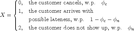
Redefine 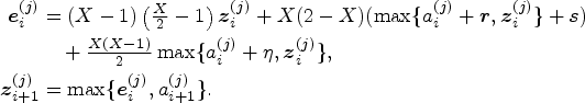
Fundamentally, due to the assumption that customers are homogeneous, albeit with additional diversity in their behaviors, all theorems remain valid, as confirmed by the following corollary.
With the consideration of last-minute cancellations, late arrivals, and no-shows, Remark
In this section, we first develop a dynamic programming (DP) algorithm for dealing with online FCFS appointment scheduling. Subsequently, we simplify the DP algorithm to address offline problems. These two cases can provide some basic bounds for solving online nonsequential scheduling problems. In this section, we employ
DP for Online FCFS Scheduling
Under the FCFS rule, the expected waiting time of the
Then, we can rewrite the objective function (6) as an expression of the expected waiting cost contributed by each customer, as follows:
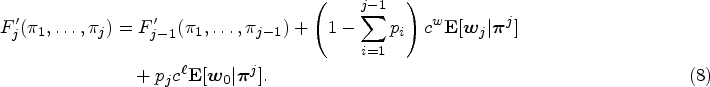
In the FCFS scheduling problem, given a partial FCFS policy
Consider a partial FCFS policy
The value
In the FCFS scheduling problem, given a partial policy
Lemma 1 can be enhanced as the following corollary, which implies that the larger the value of
In FCFS scheduling, given a partial policy 
The purpose of constructing the policy 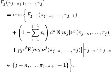
Given the schedule from the
The boundary condition of the DP is

In the above DP formulation, there are
The DP algorithm yields a cost denoted as
For a specific choice of
Lemma 3 shows that the DP value is a lower bound for the actual expected cost of the DP policy.
In addition, we note that the optimal cost of the online FCFS problem can be constrained by the DP value and the actual cost of the DP policy, as demonstrated in Theorem 4. By leveraging these upper and lower bounds, we can assess the performance of the DP algorithm. Please refer to Appendix EC.2 of the Supplemental Material for a detailed evaluation.
For a specific choice of
Since the online FCFS problem is a special case of the online nonsequential problem, the actual cost of the DP policy in the online FCFS problem
In an offline scheduling problem, the number of customers
The recursion formulation of the simplified DP algorithm is as follows:
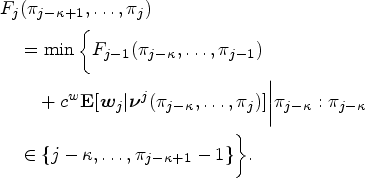

Here, the DP algorithm also provides a DP policy and a DP value. With Lemma 4, we demonstrate that the DP value, denoted as
For a specific choice of
Such a bound can be applied to our B&B algorithm, which is discussed in detail in the next section.
In this section, we begin by presenting the structure of the B&B tree. Then, in Sections 5.2 and 5.3, we propose a set of elimination rules and a lower bound. Furthermore, we provide a pseudo-code algorithm and an illustrative example to demonstrate the workings of the B&B tree. Lastly, in Section 5.5, we propose a greedy algorithm to address the challenges posed by larger problem instances, which may be difficult to solve using the B&B algorithm. In addition, in Appendix EC.1 of the Supplemental Material, we outline other contributions derived from the shortest path model.
Algorithm Description
The B&B algorithm searches for an optimal policy over a search tree. Each node in the tree corresponds to a partial policy
The B&B algorithm dynamically constructs the tree in the search process, following a best-and-depth first strategy. Once a node is generated, it undergoes a check to determine whether it violates any elimination rules. If violations are found, the node is promptly eliminated without exploring its child nodes. In addition, at each node, an evaluation is performed to estimate the lower bound cost of all leaf nodes derived from that specific node. If the lower bound exceeds the current upper bound, the node is immediately fathomed. The initial upper bound of the search tree is set as the actual cost of the DP policy developed in Section 4.1. During the search process, if a leaf node has a cost lower than the current upper bound, the upper bound is updated accordingly.
Elimination Rules
In order to enhance the efficiency of the search process, we develop a set of rules to eliminate nodes dominated by other nodes so that the remaining nodes can still lead to an optimal policy.
In light of the optimal conditions outlined in Theorem 1, we examine two sibling nodes
For any two sibling nodes
To employ Rule 1, we sort all the child nodes of a parent node in ascending order according to their state costs. This enables us to eliminate, on average, half of the child nodes, which corresponds to the best-first strategy.
In Theorem 2 and Corollary 1, we prove that within an optimal policy
If the marginal cost of a node
In Theorem 3, we show that when considering two subpaths
For a node
During the search process, when considering a specific node
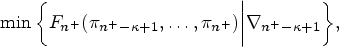
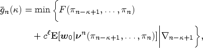
In addition to the aforementioned node elimination rules, we propose a lower bound on the cost of any full policy derived from node
First, as per Corollary 1, the condition
Second, we can derive a lower bound for
Hence, we can formulate the lower bound of 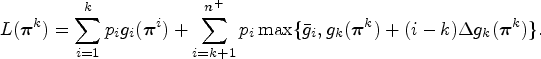
For any leaf node
During our search process, for any node
By integrating the B&B tree structure outlined in Section 5.1, the rules from Section 3.2, and the lower bound proposed in Section 5.3, we demonstrate the entire B&B algorithm with the pseudo-code provided in Appendix EC.10 of the Supplemental Material. In addition, with reference to the shortest path model, we define second-level nodes to mitigate certain redundancies associated with the root node, as shown in Appendix EC.1.2.1 of the Supplemental Material.
Throughout the search process, each node undergoes an initial assessment based on Rule 1 and, should it violate this rule, it is promptly eliminated. Among the remaining nodes, including second-level nodes, any node that fails to comply with the increasing marginal cost property specified in Rule 2 is discarded. In addition, if the partial cost
Consider a server with Search tree of the branch-and-bound (B&B) algorithm for Example 6.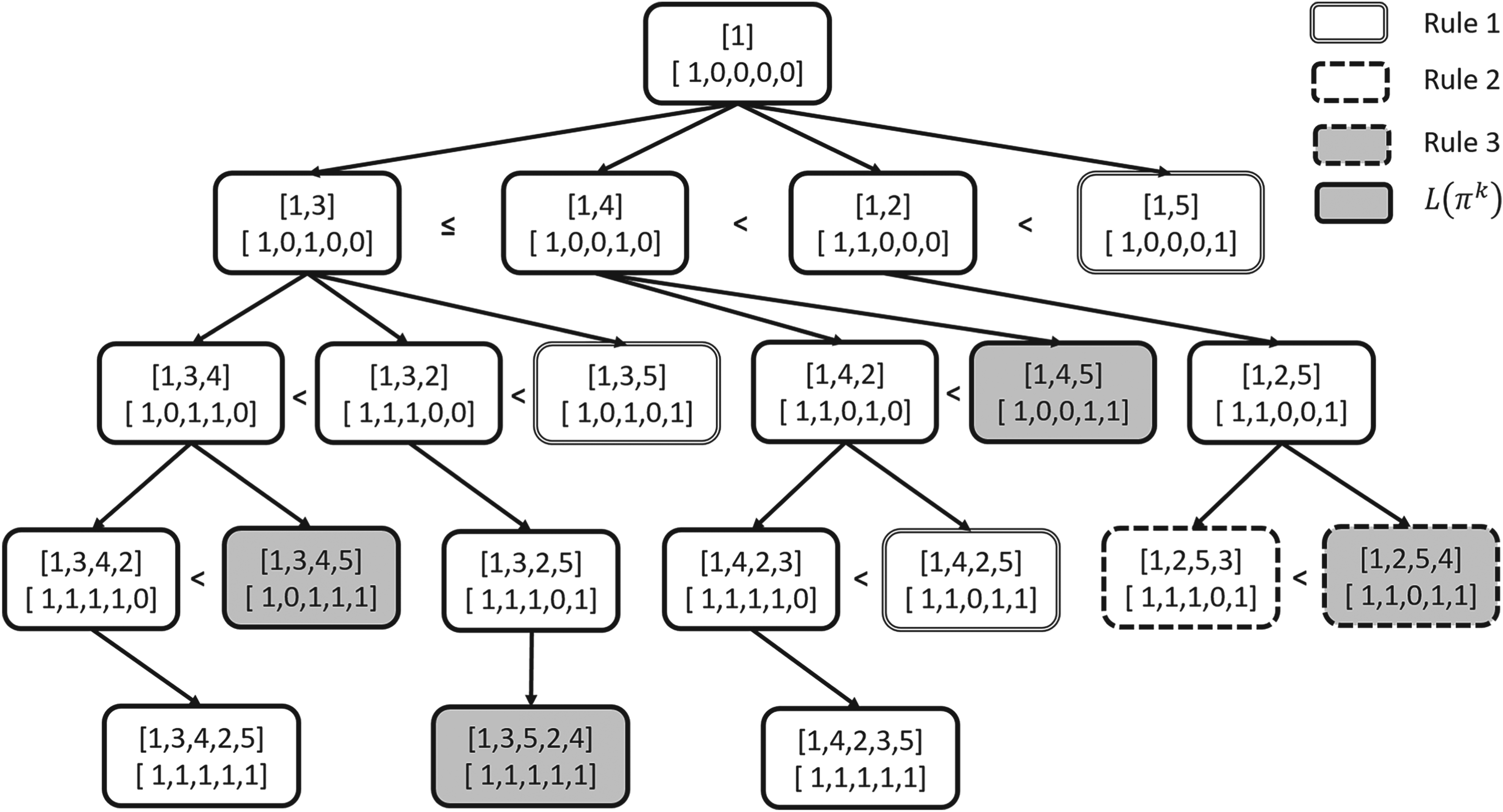
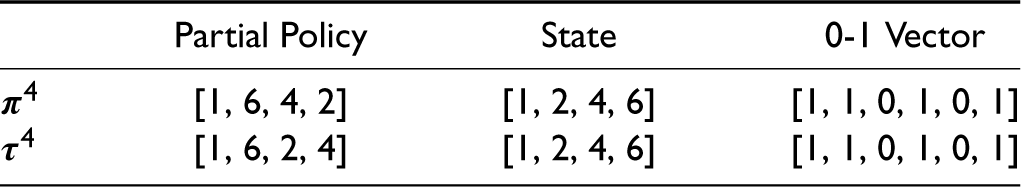
In Figure 4, each node is characterized by two descriptions, namely, the partial policy and the 0-1 vector form state. To illustrate, consider a second-level node denoted as
Within the search tree, the second-level nodes are
In Figure 4, nodes with double lines are eliminated according to Rule 1. For example, the second-level node
For large-sized instances, the B&B algorithm may be terminated once the specified time limit is reached. Consequently, we introduce a more time-efficient greedy algorithm based on the B&B algorithm.
Within the greedy algorithm, we selectively retain only the best child node from each explored node within the search tree. Since there are no sibling nodes, the application of Rule 1 is redundant. Nevertheless, we can still employ Rule 2, Rule 3, and the lower bound
Consider the instance of Example 6. We involve all the second-level nodes and show the search tree of the greedy algorithm in Figure 5. In Figure 5, the gridded nodes are eliminated via the greedy selection and only the node with the smallest state value among the sibling nodes is retained for further consideration. While Rule 1 does not apply, both Rule 2 and Rule 3 remain effective in the greedy search process. In Example 6, the greedy algorithm successfully identifies the two optimal policies. Furthermore, in Section 6, we evaluate the performance of the greedy algorithm when applied to large-scale instances.
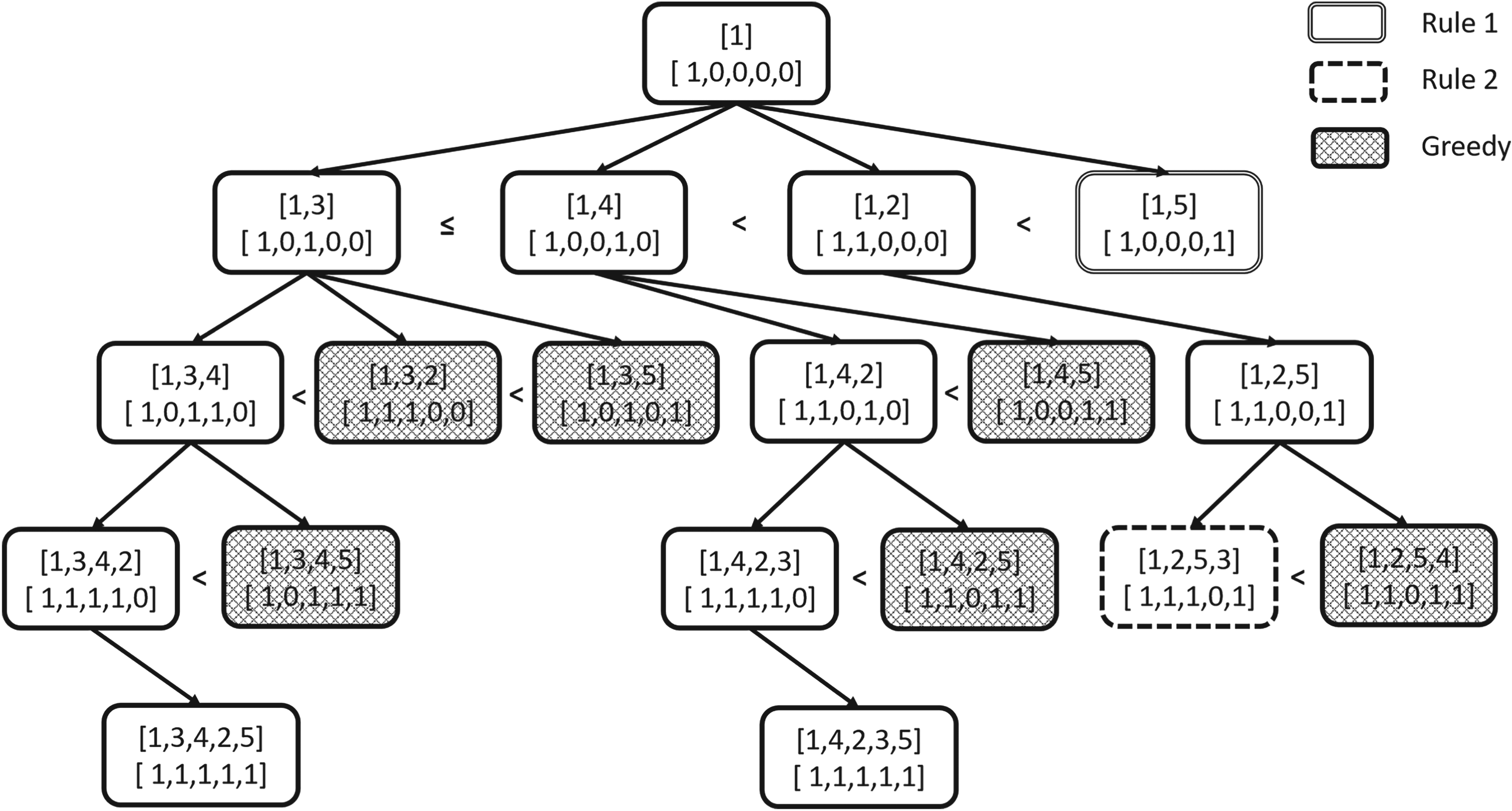
Search tree of the greedy algorithm for Example 6.
Our computational studies serve several purposes. First, we demonstrate the computational efficiency of our B&B algorithm in online nonsequential scheduling. Second, we assess the performance of our greedy algorithm when confronted with large-scale problems. Third, we study the benefit of nonsequential policies compared to FCFS policies. Fourth, we delve into the impact of last-minute cancellations, late arrivals, and no-shows. Fifth, we investigate the competitive ratio (CR) between implemented online nonsequential policies and offline policies. Sixth, we compare heuristics proposed by existing papers with the optimal nonsequential policies. All the algorithms mentioned above were coded in Python and tested on a desktop computer with an i7-7600 CPU.
The instances used in our computational studies are as follows. By default, the service horizon is designated as
In our numerical studies, the mean of the number of customers, denoted as 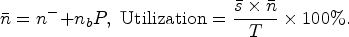
Computational Efficiency of the B&B Algorithm
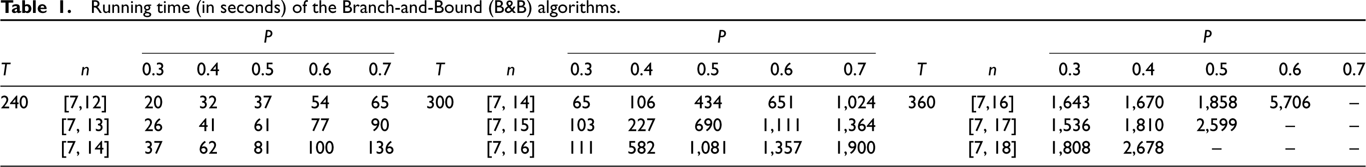
We investigate the computational efficiency of the B&B algorithm by demonstrating the computation time of the algorithm. According to the computation time presented in Table 1, we observe that our B&B algorithm efficiently solves instances with a service horizon of
Running time (in seconds) of the Branch-and-Bound (B&B) algorithms.
Running time (in seconds) of the Branch-and-Bound (B&B) algorithms.
The computation time increases as the range of uncertainty in the number of customers
In addition, we examine the percentage of retained nodes at each level using three specific instances (see Appendix EC.3 of the Supplemental Material). This analysis serves to showcase the notable efficacy of our suggested elimination rules in expediting the search process.
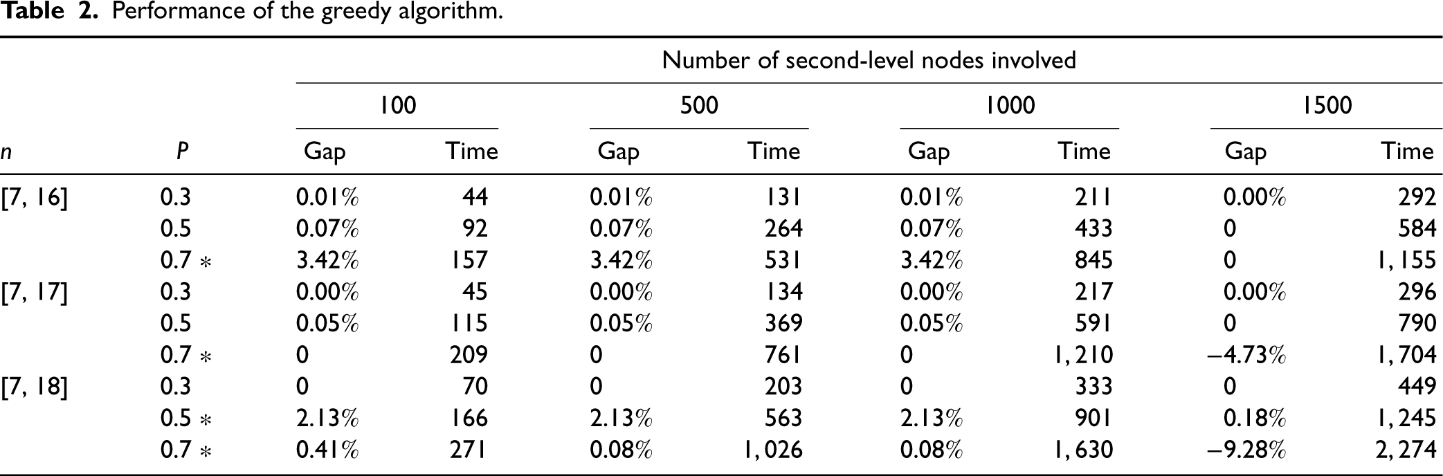
In Section 5.5, we introduce a greedy algorithm to solve large-sized instances. In this section, we evaluate the performance of the greedy algorithm by measuring the relative difference, referred to as the “relative gap,” between the cost of the policy found by the greedy algorithm and the cost generated by the B&B algorithm, with respect to the latter’s cost.
Specifically, we analyze nine large-sized instances with a service horizon of
Performance of the greedy algorithm.
Performance of the greedy algorithm.
For instances that can be solved optimally by the B&B algorithm, the gap is satisfactorily small even when applying only
In summary, the greedy algorithm is an accurate and efficient heuristic for addressing large-sized online nonsequential appointment scheduling problems.
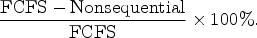
We assess the benefit of the nonsequential scheduling policy in comparison to the sequential scheduling policy and quantify it using the following expression:
Our initial inquiry explores the correlation between the benefit and two parameters pertaining to the distribution of
Benefits of nonsequential scheduling compared to sequential scheduling.
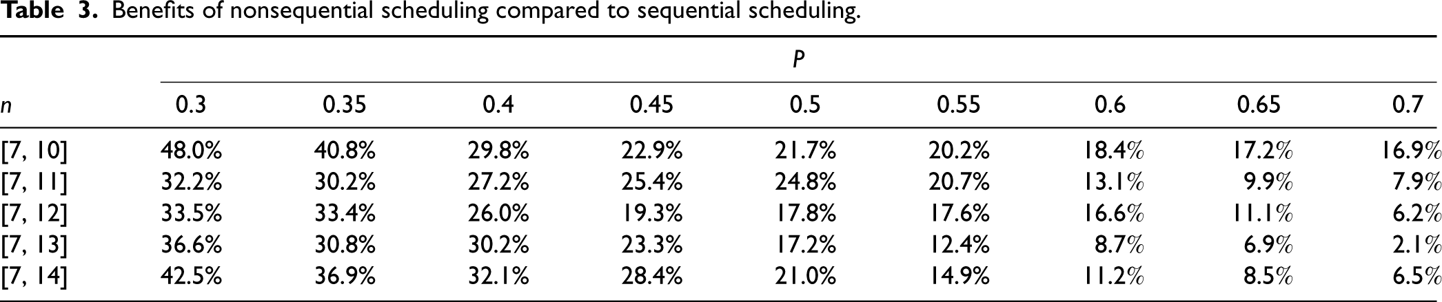
Benefits of nonsequential scheduling compared to sequential scheduling.
Benefits of nonsequential scheduling under different variances.
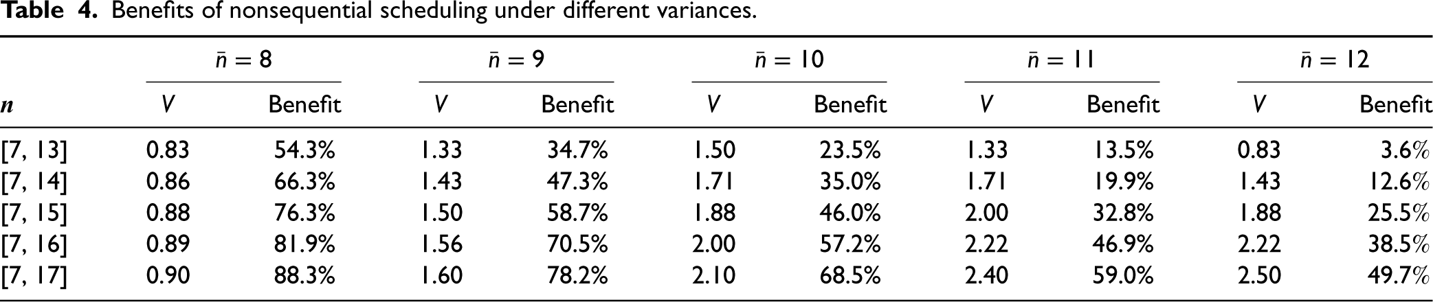
Next, we delve deeper into the association between the benefit and the combined impact of
First, given a fixed variance
Second, we explore the impact of variance on the benefit while considering a fixed mean value
In summary, nonsequential scheduling holds a significant advantage over sequential scheduling when the system is not congested or when there is a considerable fluctuation in the number of customers.
In Section 3.4, we extended our model to incorporate last-minute cancellations, late arrivals, and no-shows in the context of online intraday appointment scheduling problems. In this section, we further investigate the impact of different sources of uncertainty on online scheduling.
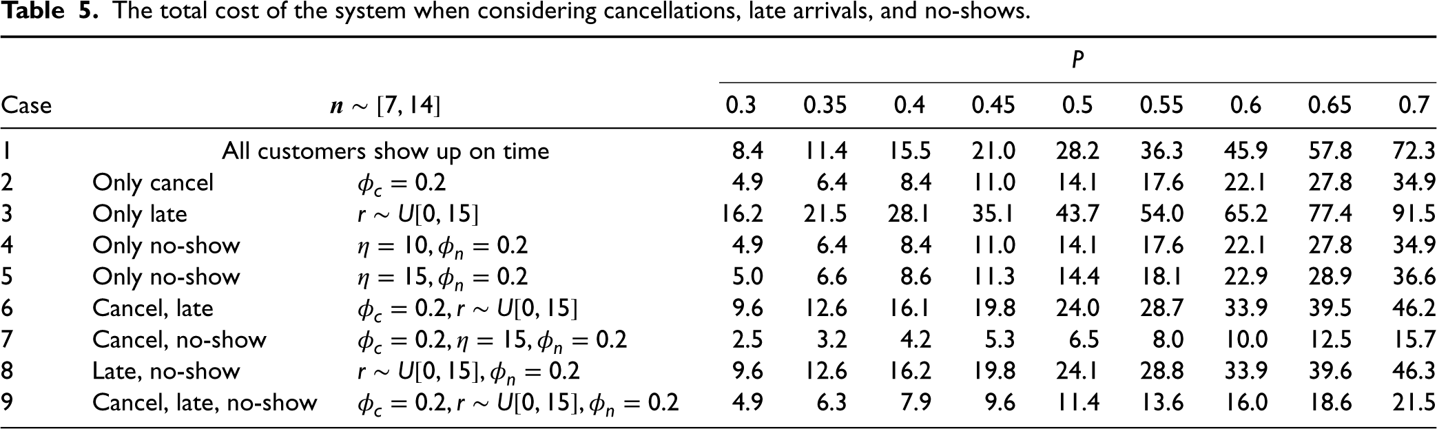
Table 5 presents the system costs in nine scenarios, including cancellations only, no-shows only, lateness only, all possible combinations of pairs, and a full complement of all three factors. The minimum and the maximum number of customers are denoted as
The total cost of the system when considering cancellations, late arrivals, and no-shows.
The total cost of the system when considering cancellations, late arrivals, and no-shows.
In Case 4, where
In summary, lateness yields a significant increase in system costs, whereas last-minute cancellations and no-shows can reduce system costs on that specific day. Furthermore, it is reasonable to treat last-minute cancellations and no-shows as interchangeable occurrences in some cases.
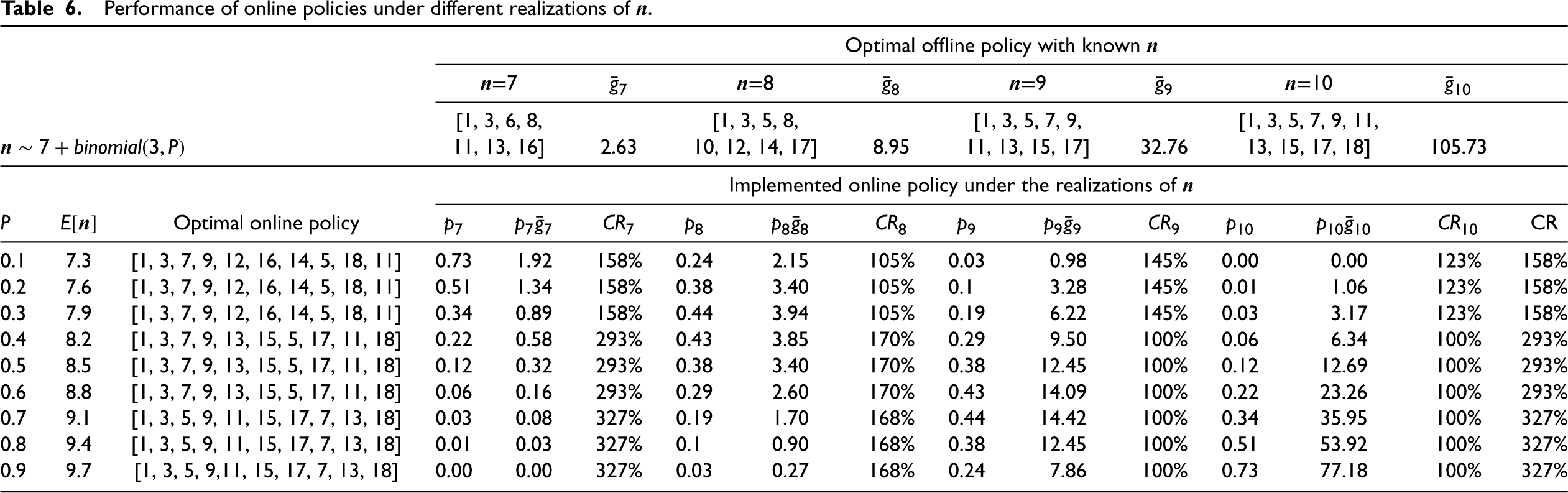
In this article, our objective is to minimize the expected cost of the system, which is a reasonable criterion given that the system knows the customer distribution. In the realm of online appointment scheduling, two additional types of evaluation criteria, namely, (i) regret analysis and (ii) CR analysis, are commonly employed to evaluate the worst-case guarantees of online policies when the distribution of the number of customers is unknown (Zhalechian et al., 2022; Stein et al., 2020). In this section, we compare the implemented optimal online nonsequential policies with their corresponding optimal offline policies, thereby assessing the performance of online policies through CR analysis. We define 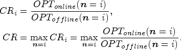
Performance of online policies under different realizations of
.
Performance of online policies under different realizations of
From the table, we observe some intriguing phenomena. First, the optimal online policy remains consistent across cases with varying
In addition, we identify certain corresponding patterns between implemented online policies and offline policies. In general, when the system is not congested, such as at
Overall, for an optimal online policy, we can always find an implemented online policy that is close to or even identical to the corresponding optimal offline policy. The point at which this correspondence appears is closely related to the expected number of customers, the customer number with the highest probability, and the maximum weighted offline cost. This corresponding pattern motivates us to leverage multiple offline optimal policies to approximate an online policy.
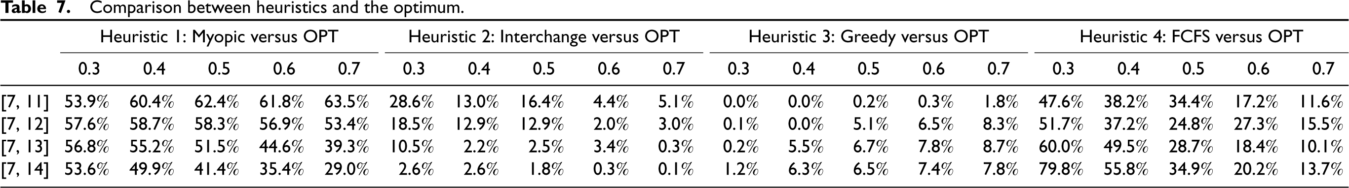
We further compare the optimal online nonsequential policies with four heuristics, as illustrated in Table 7. The first heuristic we examine is myopic scheduling (Zacharias and Pinedo, 2014). In this approach, customers call one by one, and once a customer calls, the system schedules a local optimal appointment for them immediately, regardless of possible future arrivals. The second heuristic is the pairwise interchange (Chen and Robinson, 2014). The search procedure for a nonsequential policy starts with the FCFS policy and then checks whether a pairwise interchange can reduce the cost. In each iteration, we keep the first interchange that leads to an improvement, move to a new sequence, and start afresh until no further improvement can be made. The third and fourth heuristics are the greedy algorithm and the online FCFS policy discussed above.
Comparison between heuristics and the optimum.
Comparison between heuristics and the optimum.
Of the four heuristics evaluated, the pairwise interchange and the greedy algorithm perform best, each showcasing distinct strengths. The pairwise interchange heuristic is particularly well-suited for congested systems, aligning with the observations made in the study conducted by Chen and Robinson (2014) on healthcare systems characterized by a high workload. Conversely, when the system is not crowded, the greedy algorithm demonstrates greater effectiveness. Thus, the pairwise interchange and the greedy algorithm can complement each other adeptly, and combining these two heuristics results in a well-performing heuristic that is suitable for general service systems.
Moreover, although both myopic scheduling and greedy algorithms yield locally optimal decisions in the immediate context, their overall performance diverges considerably. This observation implies that a policy that appears optimal for the first few customers may not be optimal for the system.
We study a fundamental online nonsequential scheduling problem with a random number of requests. Furthermore, our model incorporates customer cancellations, late arrivals, and no-shows, thus providing a comprehensive representation of real-world scenarios. To tackle this problem, we first investigate the online FCFS scheduling problem, which serves as a benchmark and provides an upper bound for optimal nonsequential scheduling. Subsequently, we introduce an innovative approach by integrating a dynamic assignment model and a shortest path model to develop an efficient B&B algorithm. This algorithm incorporates several elimination rules and introduces a lower bound to expedite the search process.
Through numerical studies, we assess the performance of our algorithms across different scenarios. The B&B algorithm is efficient enough to be applied to the daily appointment operations of a service system, such as 24 slots of length
Our computational study not only demonstrates the commendable performance of the proposed nonsequential policy but also several managerial insights. First, we point out situations where the adoption of nonsequential scheduling is more appropriate, namely in systems with highly fluctuating number of customers or in systems that are not congested. Second, we unveil the distinctive impacts of lateness, cancellations, and no-shows on the system. Patient lateness exerts a substantial increase in system costs, whereas cancellations and no-shows bring a certain degree of cost reduction for the given day. Through the competitive analysis, we observe a correspondence between an implemented online policy and an offline policy, suggesting that we can employ several optimal offline policies to approximate the online policy. Regarding the performance of heuristics, the pairwise interchange is more suitable for congested systems, while the greedy algorithm is more effective in relatively idle systems. The combination of these two heuristics is a well-performing heuristic suitable for general service systems. In addition, the result that the greedy algorithm outperforms myopic scheduling shows that a policy that is optimal for the first few customers is not necessarily optimal for the entire system.
Our work has limitations and future research will be valuable in several ways. First, evaluating overbooking in an online setting is valuable, where customers may have the same appointment time. Second, it would be interesting to study online appointing problems involving heterogeneous customers, such as different service time distributions. Note that in such a case, it is necessary to employ a dynamic policy that updates beliefs regarding future arrivals when scheduling real-time requests. Third, providing multiple choices to customers (Liu et al., 2019) has emerged as a new trend in online appointment problems, presenting an interesting direction for future research.
Supplemental Material
sj-pdf-1-pao-10.1177_10591478231224926 - Supplemental material for Nonsequential Appointment Scheduling With a Random Number of Requests
Supplemental material, sj-pdf-1-pao-10.1177_10591478231224926 for Nonsequential Appointment Scheduling With a Random Number of Requests by Yan Zhu, Zhixin Liu and Xiangtong Qi in Production and Operations Management
Footnotes
Acknowledgments
The authors sincerely thank the Senior Editor and two anonymous reviewers for their constructive comments that have substantially improved the quality of this work.
Declaration of Conflicting Interests
The author(s) declared no potential conflicts of interest with respect to the research, authorship, and/or publication of this article.
Funding
The author(s) disclosed receipt of the following financial support for the research, authorship, and/or publication of this article: The work is partially supported by Hong Kong RGC CRF (Grant No. C6103-20G).
Notes
How to cite this article
Zhu Y, Liu Z and Qi X (2024) Nonsequential Appointment Scheduling With a Random Number of Requests. Production and Operations Management 33(1): 184–204.
References
Supplementary Material
Please find the following supplemental material available below.
For Open Access articles published under a Creative Commons License, all supplemental material carries the same license as the article it is associated with.
For non-Open Access articles published, all supplemental material carries a non-exclusive license, and permission requests for re-use of supplemental material or any part of supplemental material shall be sent directly to the copyright owner as specified in the copyright notice associated with the article.