
Abstract
This paper explores the computational modeling of nonlocal strain, damage, and fracture in concrete, considering the isolated contribution of two random, spatially variable properties related to the fracture process: Young’s modulus (E) and tensile strength (ft). Applying a continuum damage model, heterogeneous specimens of concrete with random and spatially varying E or ft were found to produce substantial differences when contrasted with traditional homogeneous (non-random) specimens. These differences include variable and uncertain strain and damage, wandering of the failure paths, and differing (sometimes lower) peak forces, i.e. increased probabilities of failure in the heterogeneous specimens. It is found that ft variability contributes more (from 1.7 to up to 4 times more, depending on the parameter) to the overall performance variability of the concrete than E variability, which has a comparatively lower contribution. Performance is evaluated using (1) force-displacement response, (2) individual, average, and standard deviation maps of non-local strain and damage, (3) fracture paths and strain and damage values along the fractures. The modeling methodology is illustrated for two specimen geometries: a square plate with a circular hole, and an L-shaped plate. The computational results correlate well with reported experimental data of fracture in concrete specimens.
Introduction
Many engineering and infrastructure materials result from mixing dissimilar components, and consequently they exhibit a probable range of physical and mechanical properties, as well as a natural degree of randomness. In hydraulic concrete, for instance, rocks, cement, and air all have different characteristic responses to mechanisms such as load applications, temperature and moisture transfer, volume variations due to temperature changes, rates of chemical degradation, and susceptibility to specific environmental agents, among others. The coexistence of such heterogeneity within the same material plays a vital role in explaining the variability of damage and failure/fracture processes in concrete. Consequently, we intend to include randomness and heterogeneity (particularly that of modulus and tensile strength) as a part of a computational model of concrete, to study how this material performs to damage and failure while producing variable results. We will assess the random behavior of fracture paths, through analyses of strain and damage occurring in several concrete specimens, and through the study of the force sustained by this material.
The computational modeling of damage and fracture in cement-based concrete, a quasi-brittle material, has been approached through discrete and phase-field methods. Discrete methods, such as the extended finite element method (X-FEM) (Moes and Belytschko, 2002; Moes et al., 1999), cohesive zone models (CZM) (Ferte et al., 2016; Park and Paulino, 2011), and the virtual crack closure technique (VCCT) (Irwin, 1957), are based on the theory of linear fracture mechanics to integrate the discontinuities into the primary field variables; they incorporate fracture through a traction-separation law. For example, VCCT is used commonly for delamination modeling (Valvo, 2012) and benchmark configurations such as the composite double cantilever beam; a comparative approach of the X-FEM, CZM, and VCCT methods can be found in the study by Heidari-Rarani and Sayedain (2019). Discrete methods are robust for tracking and modeling macro-cracks, but they require initiations of cracks and ad hoc criteria to predict ongoing crack orientation. These requirements may limit the applicability of discrete approaches when, for instance, modeling heterogeneous materials with relatively complex geometry where multiple cracks may appear, since it may become difficult or impractical to impose the initial cracks a priori. On the other hand, the family of phase-field methods (Ambati et al., 2014; 2015; Francfort and Marigo, 1998; Sargado et al., 2018) considers brittle and ductile fractures as a continuous field where the internal states of material integrity are described by a “phase” parameter. The fracture propagation in phase-field methods is governed by minimization of an energy function, implying that diffusive cracks grow along a path which results in the least potential energy of the structure. Phase-field methods are therefore able to remedy and alleviate several difficulties of the discrete approaches. Nevertheless, it is important to remark that these methods require the phase variable to be coupled to the field of primary variables (e.g. displacements), resulting in higher number degrees of freedom, and therefore increased computational effort.
As followed by other studies closer to the behavior of interest herein, the nonlocal continuum approach is suitable for modeling damage in quasi-brittle and heterogeneous materials such as concrete (Bazant, 1994; Mazars and Pjaudier-Carbot, 1989). Due to their naturally complex compositions, these materials exhibit significantly different behaviors under tensile and compressive loading conditions. Smeared damage approaches (Comi and Perego, 2001; Kuhl et al., 2000) describe the material degradation by distinguishing damage parameters, controlled by separated tensile and compressive strain components. While highly accurate, they lead to complicated modeling and high computational costs. To tackle this issue, scalar damage models (Peerlings et al., 1996; Verhoosel et al., 2011) deal with this complexity by introducing a single damage parameter, which is in turn driven by a scalar nonlocal equivalent strain value. This variable plays the role of an indicator for the intensity of the strain tensor, considering different behaviors in tensile and compressive directions. At the same time, the evolving nature of nonlocal interactions of micro-defects is essential in the modeling of damage propagation (Pijaudier-Carbot et al., 2004; Simone et al., 2004). The progress of damage in the material is associated with volume variation in cracks and voids during the fracture process; this phenomenon has been measured experimentally for concrete using X-ray CT (Yang et al., 2017). Damage propagation has been addressed analytically by some studies (Giry et al., 2011; Poh and Sun, 2017) which have proposed appropriate laws to capture the nonlocal interactions precisely. Besides the studies in cement-based concrete, the behavior of fracture in polymer concrete, which is not the focus of this article, has also been addressed by Aliha et al. (2012).
Building from the current state of both challenges and research efforts, Nguyen et al. (2018) recently presented a model that applies a modified evolving anisotropic non-local gradient parameter to accurately calculate non-local interactions of damage micro-processes, thus addressing the issues mentioned before. This model was initially developed for and applied to homogeneous materials, and in the present study it has been selected and adapted to consider the heterogeneity and randomness of the spatially varying material properties of concrete.
Many of the studies on fracture in concrete are based on the principles of micromechanics, and thus they rely on geometric representations of heterogeneity, i.e. aggregate particles or air voids embedded in the mortar phase. For instance, recent applications (Heidari-Rarani and Bashandeh-Khodaei-Naeini, 2018; Yilmaz and Molinari, 2017) consider the modeling of rocks within the mortar phase, modeling aggregates as two or three-dimensional ellipses or spheres, and make use of the theory of cohesive zones to model fracture. Others present a detailed scanning and modeling of air voids (Han et al., 2018) and apply a crack phase field model to study the development of damage. For example, an approach using reconstructed microstructures for the study of fracture in concrete due to freeze-thaw is presented by Dong et al. (2018). Alternative approaches include discrete elements as well (Suchorzewski et al., 2018). On the other hand, some applications (Guo et al., 2009) have used innovative techniques to model the material with truss-like elements (i.e. lattices) achieving a mesoscopic, ‘overall' description of fatigue damage in concrete; the microstructure is generated after a picture of a real concrete specimen. Such models of heterogeneous materials enable the analysis of dynamic responses, the appearance of fracture patterns, and in general they assess the effect of parameters such as fracture energy, fatigue damage, and aggregate/air void characteristics (shape, orientation, volume fraction). Particularly, Eliáš et al. (2015) presents fracture results of concrete beams under three-point-bending with varying notch depths, including no notch, using a microstructure-based approach to heterogeneity similar to a point to this study. Both Eliáš et al. (2015) and the present paper coincide in predicting (1) increased variability in the response of stochastic models when compared to the experimental results, and (2) lower peak forces when the specimens are random than when they are not. Additionally, the modeling approach and simulations herein are performed with the objective of isolating the influence of E and ft on the variability in performance of concrete.
Perhaps the most important difference between the present study and those mentioned before is the absence of an aggregate microstructure. Herein, aggregates are not considered explicitly because the meso-scale discretizing of concrete does not intend to represent individual rock particles. Conversely, the discretization enables a synthetic representation of the uncertainty of material properties in space. This uncertainty is reflected later in the variability of the results (Results and analysis section) and is comparable with data reported experimentally. Heterogeneous models that consider inclusions are computationally heavy (Chen et al., 2018a; You et al., 2012), and a considerable part of these elevated computational costs goes to considerations regarding the interface and contact models between the particles and the binder. The methodology presented herein intends to offer an alternative approach, using repetitive simulations with identical discretization but slight (random) differences. Not having a microstructure is precisely what makes each simulation manageable enough so that a high number of models can be set up and run, while managing to obtain results that are representative of the damage and fracture of the material. For an explicit consideration of rock aggregates and heterogeneous effects, the reader is referred to Caro et al. (2018) and Qin et al. (2020); an alternative homogenization approach can be found in Chen et al. (2018b
In this study, we isolate the contribution of modulus (E) and tensile strength (ft) of concrete to the overall variability in strain, damage, and fracture. To this end, we set up computational specimens of concrete with spatially random modulus and tensile strength. The random specimens, or plates, are subjected to controlled displacement boundary conditions that induce damage. We study the force-displacement response of the random specimens, and we provide an overview of specimen-specific and overall maps of non-local strain and damage. Finally, we study the variable behavior of fracture paths as well as the strain and damage values along the fractures. The results from the computational specimens are compared with experimental data reported previously (Winkler, 2001). The paper presents the methodology for modeling and simulation, followed by the results, analysis, and conclusions of the study.
Methodology
The methodology for modeling the spatial variability of mechanical properties of concrete can be divided into three steps, as follows:
Define the domain geometry and mesh: Two geometries were selected: holed and L-shaped (Step 1. Geometry and mesh of the domain section). Assign material properties to the mesh (repeat to create specimens): Random, spatially correlated values of Young’s modulus (E) and tensile strength (ft) are assigned Per geometry, 100 specimens have Per geometry, 100 specimens have Simulations: The 400 random specimens from Step 2 are modeled in finite elements (Step 3. Considerations for FE simulation and modeling of damage section). A controlled displacement is applied; the holed specimens are subjected to tension, and a nodal displacement is applied upwards to one corner of the L-shaped specimens. Concrete is modeled quasi-brittle and develops damage; after a strain threshold is surpassed, it becomes progressively unable to sustain load, with damage eventually spreading and inducing fracture. The following parameters are obtained and analyzed: force sustained by the specimens, non-local strains, damage, and fracture paths.
Step 1. Geometry and mesh of the domain
Two geometries of concrete are used as model structures in this study. The first geometry is a holed plate of side 200 mm with a circular inclusion. The second plate geometry is L-shaped, 500 mm high. The meshed geometries are presented in Figure 1. Details about the selection and characteristics of the geometries are provided next.
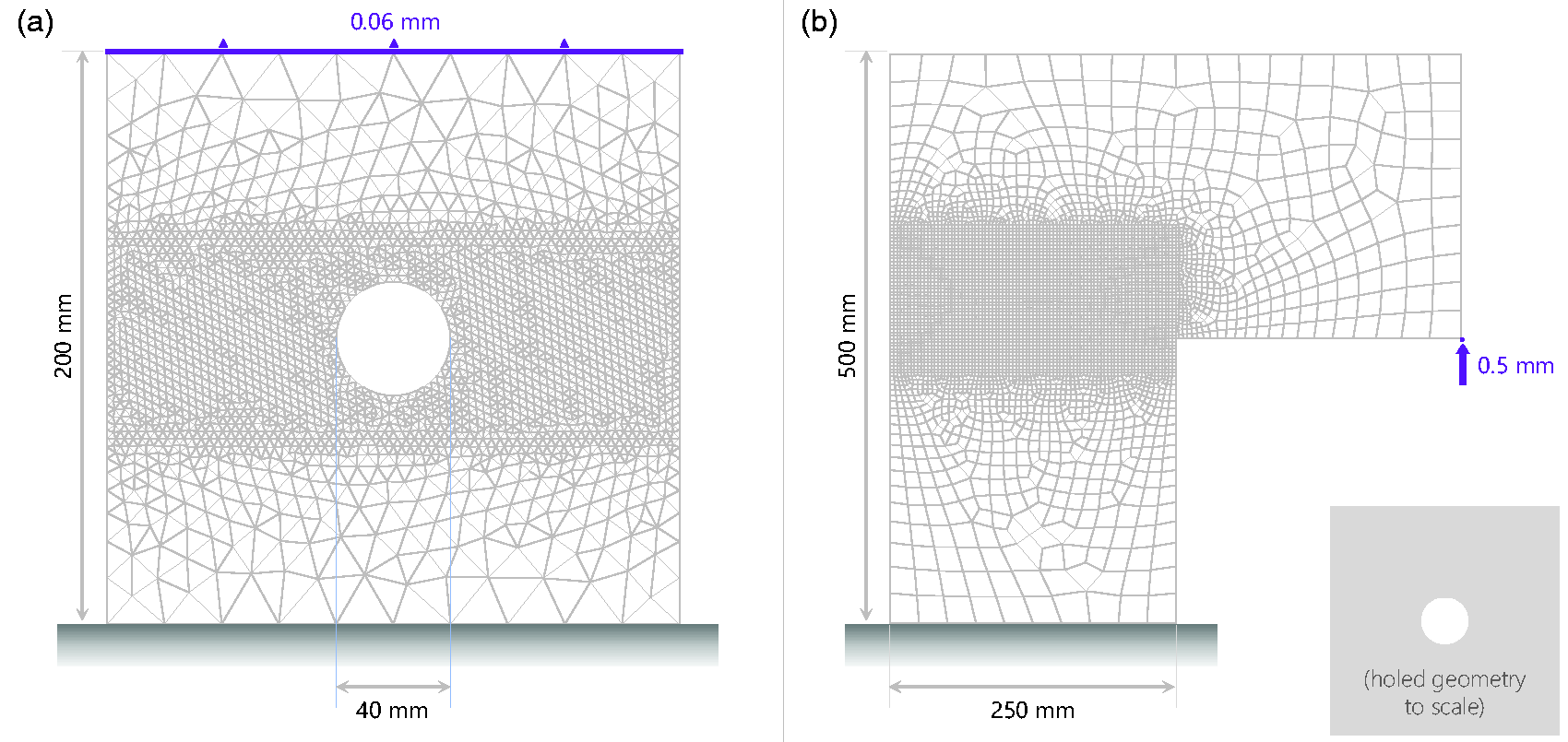
Meshed geometries and boundary conditions for (a) holed specimen, (b) L-shaped specimen. The domains are meshed with triangular and quadrilateral finite elements, respectively. Note the difference in size.
To fully capture the effects of nonlocal interactions and strain localization, finer mesh sizes are required in critical areas where high-gradient values of stress and strain are foreseen, and where damage concentration and fracture are likely. The meshes were defined after a mesh convergence analysis with finest element sizes between 2 mm (fine) and 5 mm (coarse). It was found that a mesh with an intermediate size of 3 mm is within 0.7% of the results of the finest mesh (holed geometry) and even closer for the L-shaped (within 0.1%). The selected meshes have 4,786 elements (holed geometry) and 5,306 elements (L-shaped geometry). The two geometries are created and discretized using the open-source software Gmsh (Geuzaine and Remacle, 2009).
It can be observed from Figure 1 that the mesh for the holed geometry has an uneven horizontal distribution for the nodes, i.e. the nodes do not describe a horizontal line where failure is expected. This was intentional, to avoid prescribing the expected failure path; such a mesh was tested as part of modeling trials, and even while variability still emerged, results showed a strong bias due to the mesh. On the other hand, the finer mesh for the L-shaped geometry is made of squares because failure is expected to be diagonal.
Two element types are used: the holed geometry is meshed with standard linear triangular finite elements with three nodes (T3) and the L-shaped geometry is meshed with four-node quadrilateral elements (Q4). Selecting these standard low-order finite favors simplicity while avoiding stress oscillation, as introduced in the smoothing gradient damage model (Nguyen et al., 2018).
Overall, the use of the two geometries (one with an inclusion, the other with a concave polygonal shape), two types of elements (triangular and quadrilateral), and two loading schemes (inducing different modes of fracture, see Step 3. Considerations for FE simulation and modeling of damage section) intends to show the versatility of the modeling methodology and its ability to adjust to a range of domain sizes and geometries, and element types. Additionally, results from the L-shaped geometry are compared with experimental data (Winkler, 2001) of identical material and test conditions, to support the validity of the model results.
Step 2. Random material properties
Step 2 of the methodology consists of the assignment of random, spatially correlated values of Young’s modulus (E) and tensile strength (ft) to the meshed specimens. As mentioned before, to isolate the influence of E and ft on the fracture behavior of concrete, 400 random specimens of concrete are created as follows, in four sets:
100 holed specimens have 100 holed specimens have 100 L-shaped specimens have 100 L-shaped specimens have
To have control over the spatial correlation structure of the random specimens, we use the methodology of random fields through matrix decomposition (EL-Kadi and Williams, 2000) to obtain values that are both random and correlated in space. Random fields are selected because they are a versatile stochastic tool to generate probable random vectors of numbers that are spatially correlated (Vanmarcke, 1983). These numbers can then be interpreted as values of a mechanical property of concrete. The assignment of mechanical properties is carried out element wise; that is, every finite element in the mesh is assigned an individual, unique value of E or ft that is constant within the boundaries of the finite element. There are 4,786 finite elements in the holed geometry mesh, and 5,306 elements in the L-shaped geometry mesh. This means that each of the 400 random specimens has around 5,000 random, normally distributed values of E or ft, effectively enabling the modeling of concrete as a heterogeneous material. A summary of the random, heterogeneous specimens of concrete is presented in Figure 2.
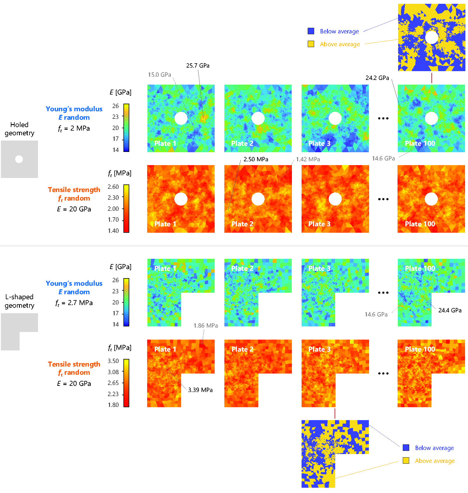
Random specimens or plates of concrete, displaying spatially correlated values of Young’s modulus (E) or tensile strength (ft). Values correspond element wise to the finite elements on the mesh (see Figure 1). Minimum and maximum values of E and ft are marked in some specimens, as well as the regions where the values of E or ft are below/above the average for the specimen. Note that the holed and the L-shaped geometries are not to scale.
Instead of the theoretical concrete material with homogeneous mechanical properties used conventionally, we now have specimens that exhibit randomness and spatial variability encompassing a range of E and ft values. Following are some characteristics that support, from the computational point of view, this synthetic representation of variability as a valid and convenient representation of real materials, depicting and encapsulating heterogeneity in an intuitive and manageable way.
Each replicate or random specimen of concrete, i.e. each configuration of E and ft, is unique and non-repeatable; however, the mean, variance and spatial correlation of E and ft along the specimens are the same for each of the four “sets”. The average of the random element-wise values of E and ft is always exact, as is their standard deviation, which was set as 7.5% of the respective average (standard deviation of E is 1.5 GPa, and of ft is 0.15 MPa for the holed geometry and 0.2025 MPa for the L-shaped geometry). The distance around any point in the meshes within which the random values of E or ft are correlated (i.e. the correlation length) was set to 25 mm. Both the standard deviation and the correlation length were selected for further evaluation and comparison with the variability of the experimental data. Relevant reference data for these parameters is scarce from the perspective of this modeling approach. The selection of values was therefore guided by typical aggregate sizes in concrete and preliminary computational testing. Nevertheless, the selection is considered reasonable as (1) the data will ultimately be contrasted with experimental results, in both homogeneous and heterogeneous (random) cases, and (2) from the modeling perspective of isolating the contribution, it is more relevant that these values remain constant among the cases.
Approximately half of the surface area of the random specimens lays below/above the average for the specimen (either E or ft), as would be expected from a real concrete specimen. In fact, element-wise values of E on any given specimen may lie anywhere between 15–25 GPa, and values of ft between 1.5–2.5 MPa (holed geometry) and between 2–3.5 MPa (L-shaped geometry), as marked in Figure 2. This is due both to the normal distribution of the random values and to the uniformity of the correlation structure throughout the random field. For the same reasons, the specimens contain relatively distinct ‘weaker’ and ‘stiffer’ areas, i.e. groups of adjacent elements where E or ft are relatively low or high. Such a computational approach may be more consistent with the laboratory experience than the traditional homogeneous simplification; for example, on a real specimen of concrete these areas could represent high/low air void concentrations, fiber reinforcement or other inclusions, deficiencies in concrete vibration, uneven presence of water during hardening, or chemical degradation, among other phenomena. In particular, the random nature and location of the weakest and stiffest areas may prove critical for processes of damage and fracture.
In the holed geometry, fracture is expected along the horizontal direction, besides the circular inclusion. Focusing on the top, left-most specimen of Figure 2 (Holed geometry, Random E, Plate 1), it can be observed that a relatively stiff area occurred to the right-hand side of the inclusion, directly across the expected fracture path. Naturally, the development of strains and damage in this specimen might be affected by this occurrence. Similar phenomena can be observed in other random specimens. The ability to consider such unique, sometimes extreme or critical cases is a key feature of the modeling methodology presented herein.
In this study, the random fields are constructed following the matrix decomposition technique. Each realization of a field is composed of random, spatially correlated values. The values are assigned to target coordinates, in this case, the center of each element. The correlation length of a random field is a generation parameter, and it holds regardless of the distance between the target coordinates (i.e. regardless of element size).
Step 3. Considerations for FE simulation and modeling of damage
Step 3 of the methodology consists of the simulation of the 400 random specimens (200 holed, 200 L-shaped) using the finite element method. Additional homogeneous specimens are created for comparison, i.e. with non-random E and ft. The full calculation procedure is depicted as a flow chart in Figure 3.
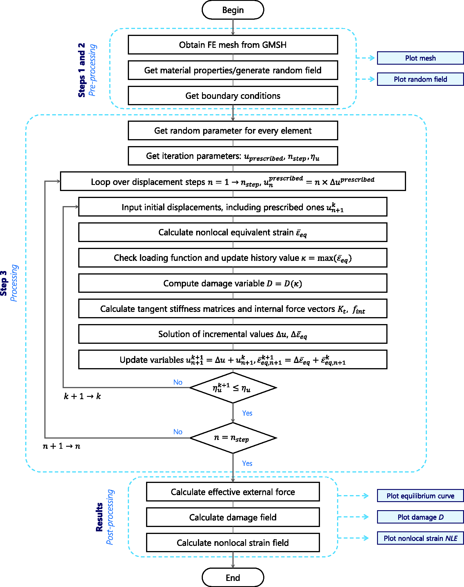
Scheme of the damage algorithm for heterogeneous materials.
The boundary conditions restrict translation and rotation of the bottom edge of the domain, while prescribed displacements are applied to the top edge (holed geometry) or a corner node (L-shaped geometry). The boundary conditions and applied displacements can be appreciated in Figure 1. As observed, they aim to induce damage/fracture mechanisms of pure tension (Mode I) and mixed. In detail, the boundary conditions are:
Holed geometry: The lower edge of the specimen is restricted from displacement. A (tensile) displacement of 0.06 mm is applied upwards, linearly and uniformly to all nodes on the upper edge. The displacement is equally prescribed for 250 steps. This displacement corresponds to 0.03% of the height of the domain. L-shaped geometry: The lower edge of the L-shape is restricted from displacement. A prescribed displacement of 0.5 mm is applied upwards, in 100 steps, to the bottom node of the ‘free’ right edge of the L-shape. This displacement corresponds to 0.1% of the height of the domain.
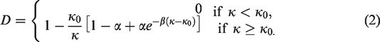
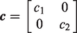
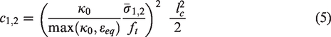
The simulation is performed using the smoothing gradient damage approach (Nguyen et al., 2018), modeling the internal variable damage (D), which represents the normalized loss of material integrity in the constitutive relation

For quasi-brittle materials like concrete, the damage evolution follows the exponential law (Peerlings et al., 1996)
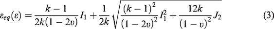
This study follows a nonlocal approach, where the damage parameter is implicitly driven by an independent field (non-local equivalent strain

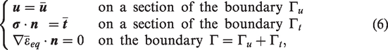
The boundary conditions are given as
The simulations are carried out via a MATLAB in-house finite element code. The code files are single-threaded and run on a personal computer with an Intel Xeon 1230v5 processor and 16 GB memory. Under the conditions of this study, one simulation takes approximately 120 minutes (holed geometry) and 60 minutes (L-shaped geometry). It is worth mentioning that a corresponding homogeneous and heterogeneous geometries have similar running times, i.e. heterogeneity does not add a cost when running the model, only when building the model.
Results and analysis
The results of the simulations of 200 holed specimens, 200 L-shaped specimens, and corresponding homogeneous specimens of concrete (one per geometry) are divided into three types and presented as follows:
Force-displacement curves: We obtain and report the calculated force-displacement paths of the random specimens under the applied boundary conditions. Strain and damage: As presented in Step 3. Considerations for FE simulation and modeling of damage section, the Fracture: The fracture paths are calculated from the nodes in the mesh where NLE and D are maximum.
The force-displacement curves are an overall result, i.e. there is a unique response curve per specimen of concrete. On the other hand, the strain, damage, and fracture paths are spatial responses calculated per element. We report the maps of NLE and D of selected specimens, as well as the overall element wise average and standard deviation results at different steps of the simulation.
Force-displacement curves
Overall results
The force-displacement (F-D) response curves were obtained at the node(s) where the displacement boundary condition was applied. Each of these curves summarizes the overall behavior of a specimen of concrete, be it random or homogeneous. A summary of all curves is presented in Figure 4: the 200 random holed specimens in Figure 4(a), and the 200 random L-shaped specimens in Figure 4(b). The associated standard deviation of the four sets of curves is shown in Figure 5.
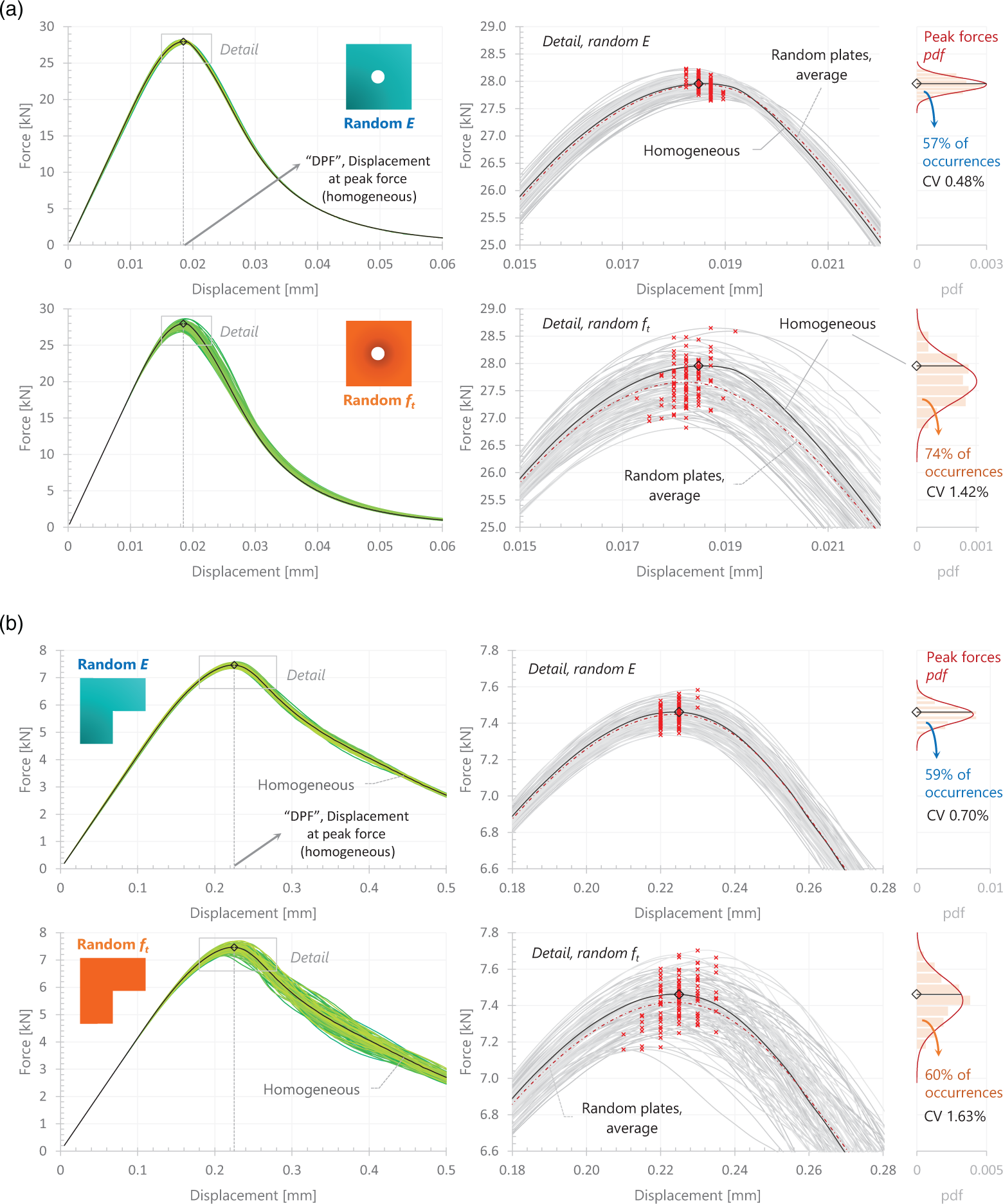
Force-displacement (F-D) curves for the random specimens of concrete under prescribed displacement. Each curve represents the response of a specimen. A detail of the peaks of the curves is shown, as well as the probability density function of the peak force values. (a) Holed geometry, (b) L-shaped geometry.
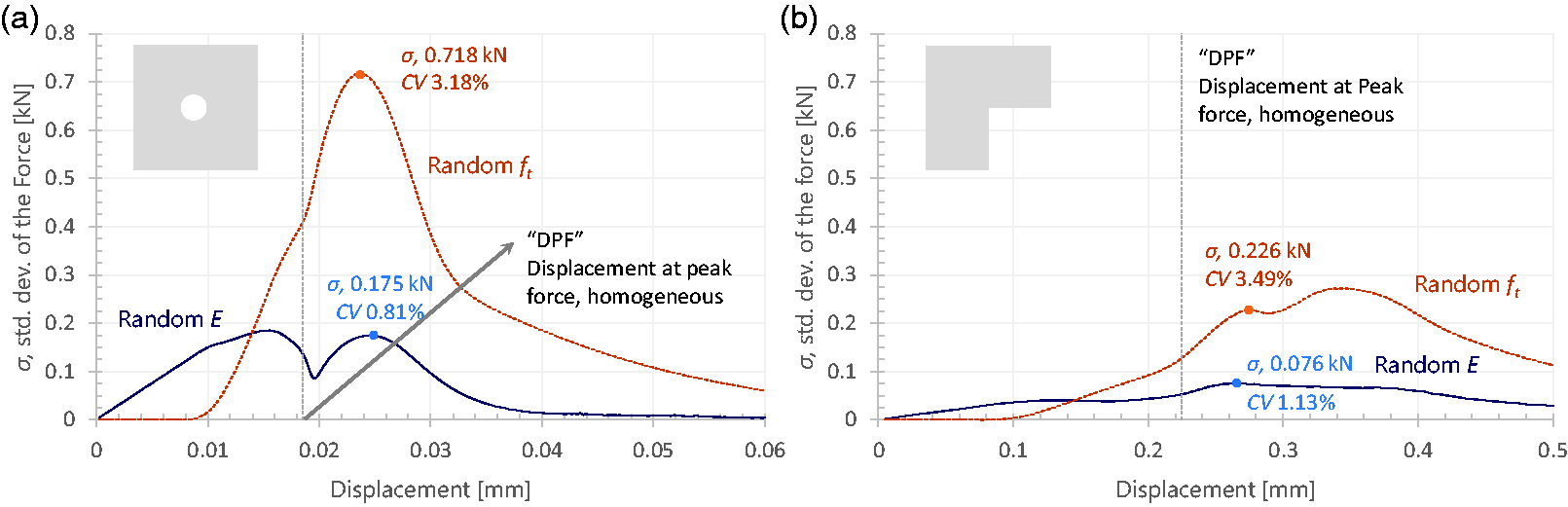
Standard deviation of the force-displacement curves in Figure 4. Vertical axis to scale. Notice the difference in scale of the Displacement axes. CV is the coefficient of variation.
The results of the simulations suggest that the spatial variability of E and ft contributes in different proportions to the overall variability of force-displacement results. In both holed- and L-shaped geometries, F-D curves of the random specimens of concrete showed considerably higher dispersion when the variability was contributed exclusively by ft. We can now quantify the difference in contribution.
At the beginning of the simulations the standard deviation (σ) of the F-D curves is zero. The F-D curves are close together, and low variability is expected initially because (a) the concrete is undamaged and responding with full integrity, (b) the average values of E and ft are constant among each set of specimens, and (c) the specimens with random ft show no variability at first, because E is constant (see Figure 5, dotted curves).
In the random-E specimens, σ increases slowly and reaches very low values, remaining below 0.2 kN (holed geometry) and 0.05 kN (L-shaped geometry) before displacement at peak force (DPF) of the homogeneous specimen. On the other hand, variability of the random-ft specimens (i.e. constant modulus) appears at a displacement ∼40% of the DPF, a clear indicator that damage has begun. Here, σ increases at a stable rate and considerably more rapidly for the random-ft than for random-E specimens, reaching 0.40 kN (holed geometry) and 0.13 kN (L-shaped geometry) at DPF, which is 2.5–3 times more than σ of the random-E specimens at the same displacement. Except for the random-E holed specimens, σ of the F-D curves increases monotonically and doubles after DPF.
The dispersion among the F-D curves reached a (local) maximum moments after DPF. At its highest, this standard deviation represents 3–3.5% (random ft) and ∼1% (random E) of the force of a comparable homogeneous specimen. At this point, the contribution of ft to F-D variability was 4 times higher (holed geometry) and 3 times higher (L-shaped geometry) than the specimens with random E. σ decreases after that point, except for the random-ft L-shaped specimens, which reach a global maximum shortly after (area of maximum dispersion; see Figure 4(b), random-ft around displacement 0.35 mm).
Identical input variability for both geometries induced a greater increase in CV (see Figure 5) between random-E and random-ft specimens; CV increased 4 times for the holed geometry and 3 times for the L-shaped geometry. Overall, the holed geometry appears to be slightly more sensitive to the variability of ft than the L-shaped geometry.
Peak force values
The behavior of the peak force values sustained by the random specimens is consistent with the previous analysis of dispersion of the F-D curves. Random-ft specimens contribute considerably more to overall variability than random-E. When the variability was contributed exclusively by ft, the coefficient of variation (CV) of the peak forces increased from 0.48% to 1.42% (holed geometry) and from 0.70% to 1.63% (L-shaped geometry) compared to random-E specimens; suggesting that ft contributed 2-3 times more than E to the variability of peak forces. The right-hand side of Figure 4 presents the frequency histogram and calculated probability density function (pdf) for the peak forces.
Some observations can be made from these results. Based on this analysis alone, the probability that a random specimen resisted a maximum (peak) force lower than a homogeneous specimen was 57% (holed geometry) and 59% (L-shaped geometry) for random E. When only ft contributed to variability, this probability increased to 74% (holed geometry) and remained similar at 60% (L-shaped geometry). Remarkably, the probability was not 50% in any case. In fact, while this calculation can be fine-tuned with a larger number of simulations, it was consistently greater than 50% for both geometries and random properties. These results suggest that a material model that considers random, spatially variable properties (in other words, heterogeneity) will estimate in average a lower response, i.e. increased probability of failure than if the material was homogeneous. This can be observed when comparing the average of the random F-D curves with the homogeneous curve around the peak forces; the random-average was lower, if only slightly, for both geometries and random properties.
An associated variability in peak force displacements was also observed. Displacement values are discrete due to the steps of the simulation. Nevertheless, the displacements at peak force showed a CV of 0.97–1.13% (random E) and 1.68-2.47% (random ft); 1.7-2 times greater due to ft variability. The maximum difference between the maximum and minimum occurring displacements at peak force amounted to ∼4% (random E) and ∼10% (random ft) of the DPF. No correlation was found between peak force sustained, and the maximum-to-minimum difference of E or ft for the random specimens.
Comparison with reported experimental results
Considering the resources required to perform and instrument laboratory tests of concrete damage and fracture, it is complicated to obtain extensive fracture data of concrete that is suitable for variability analyses. In fact, offering a computational alternative to this situation is one of the motivations of the present study. For example, recent results on crack propagation tests on concrete have been reported (Carpiuc-Prisacari et al., 2019), building an experimental database and including tests with crack bifurcations. This data was measured with advanced equipment, and digital image correlation techniques were used to capture displacement fields.
In the present study, we refer to results previously reported in the literature for L-shaped specimens of concrete under tension. The geometry, boundary and loading conditions, and material parameters of the L-shaped specimens of the present study were obtained from Winkler (2001). Figure 6 superimposes the range of experimental results (shaded area) as reported by Meschke and Dumstorff (2007), with corresponding data from our simulations; i.e. 200 L-shaped specimens. X-FEM results with the same geometry and load configuration (Meschke and Dumstorff, 2007) are also presented for comparison. Meschke and Dumstorff (2007) obtained a Young’s modulus of 25.86 GPa. However, this value seems to be overestimated, as the elastic structural response is out of the experimental zone. For this reason, herein we selected E as 20 GPa to fit the force-displacement curve in the middle of the experimental zone for the homogeneous plate (see Failure paths section).
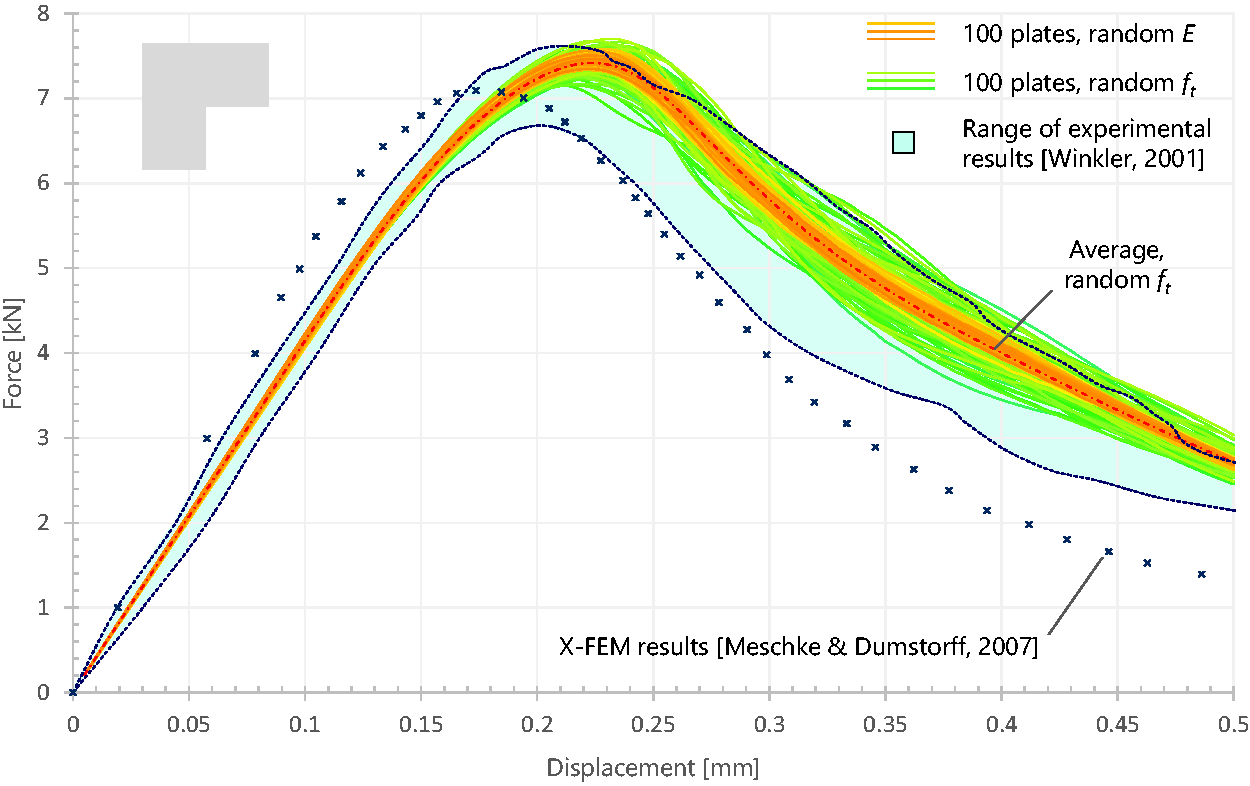
Comparison of force-displacement curves for an L-shaped domain of concrete, including experimental and numerical results. Data from the present study, Winkler (2001) as reported by Meschke and Dumstorff (2007), and Meschke and Dumstorff (2007).
As seen in the figure, the range of potential responses encompassed in this study is in line with experimental results. Even the more variable curves from the random- ft specimens lie mostly within the bounds of the experimental range; random-E specimens do almost entirely. The wider range attained by the experimental data suggests that higher input values of variability may be assumed than those proposed in the present study (7.5% CV for E and ft, see Step 2. Random material properties section) to represent the natural spatial variability of concrete. Some parameters like the correlation length may be maintained, as there is limited validation data. The post-failure behavior fits well with the data from the experiments, reaffirming the validity of the damage model used in this study. The similarity also extends to the fracture paths (see later Figure 12(a)).
Strain and damage
Selected random specimens and homogeneous results
Figures 7 and 8 present the maps of non-local equivalent strain (NLE) and damage (D) for selected random specimens of concrete, as well as the results from the homogeneous specimens. The homogeneous response is contrasted with the element-wise average of the random-E and random-ft cases.
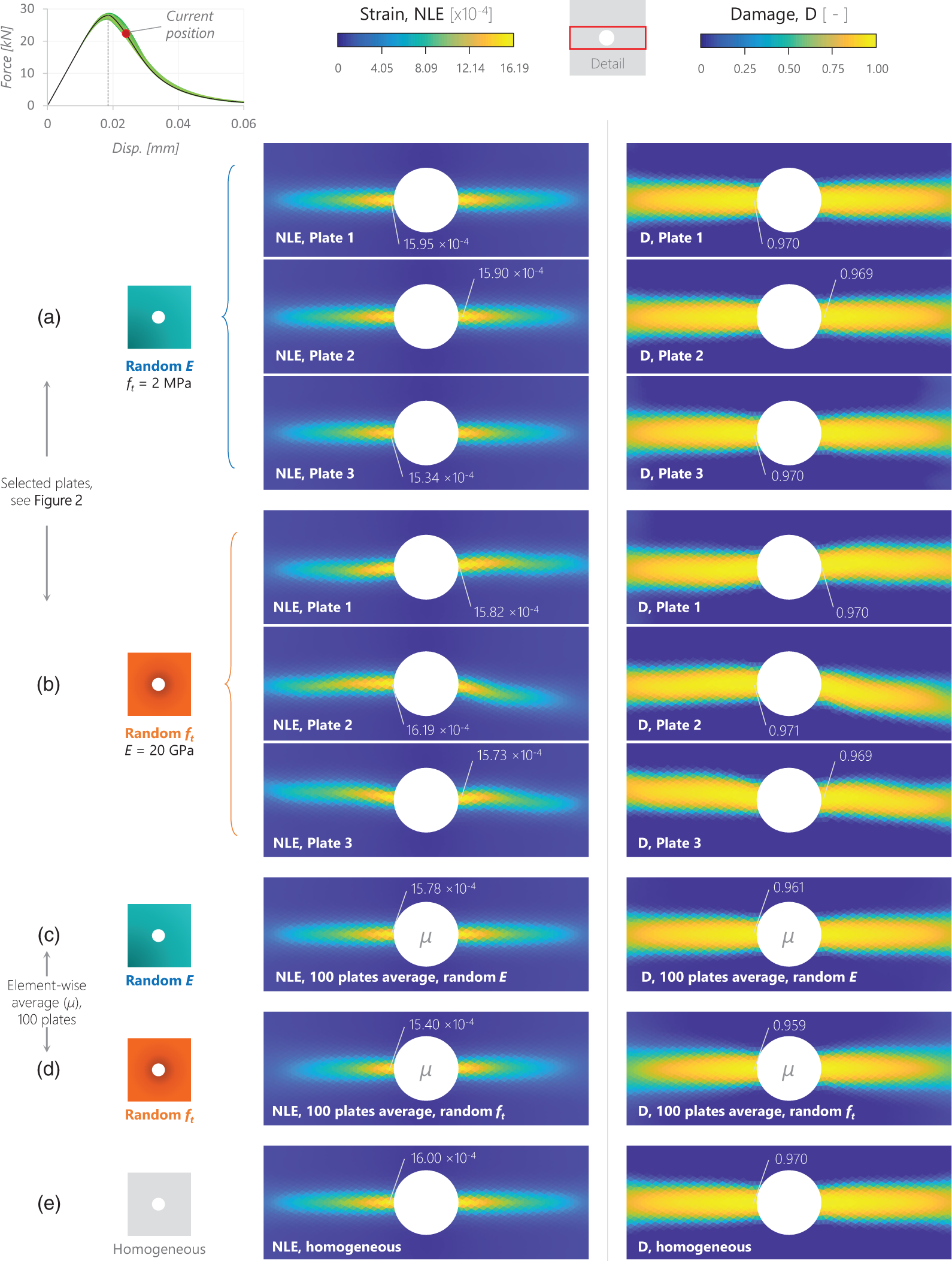
Maps of non-local equivalent strain NLE, and damage D for the holed geometry (detail). The current displacement is presented on the force-displacement curve, top left. (a) Selected random-E specimens, same from Figure 2. (b) Selected random-ft specimens, same from Figure 2. (c) Element-wise average (μ) for 100 random-E specimens and (d) 100 random-ft specimens. (e) Homogeneous specimen. Maximum values are marked. Deformation factor is 0.
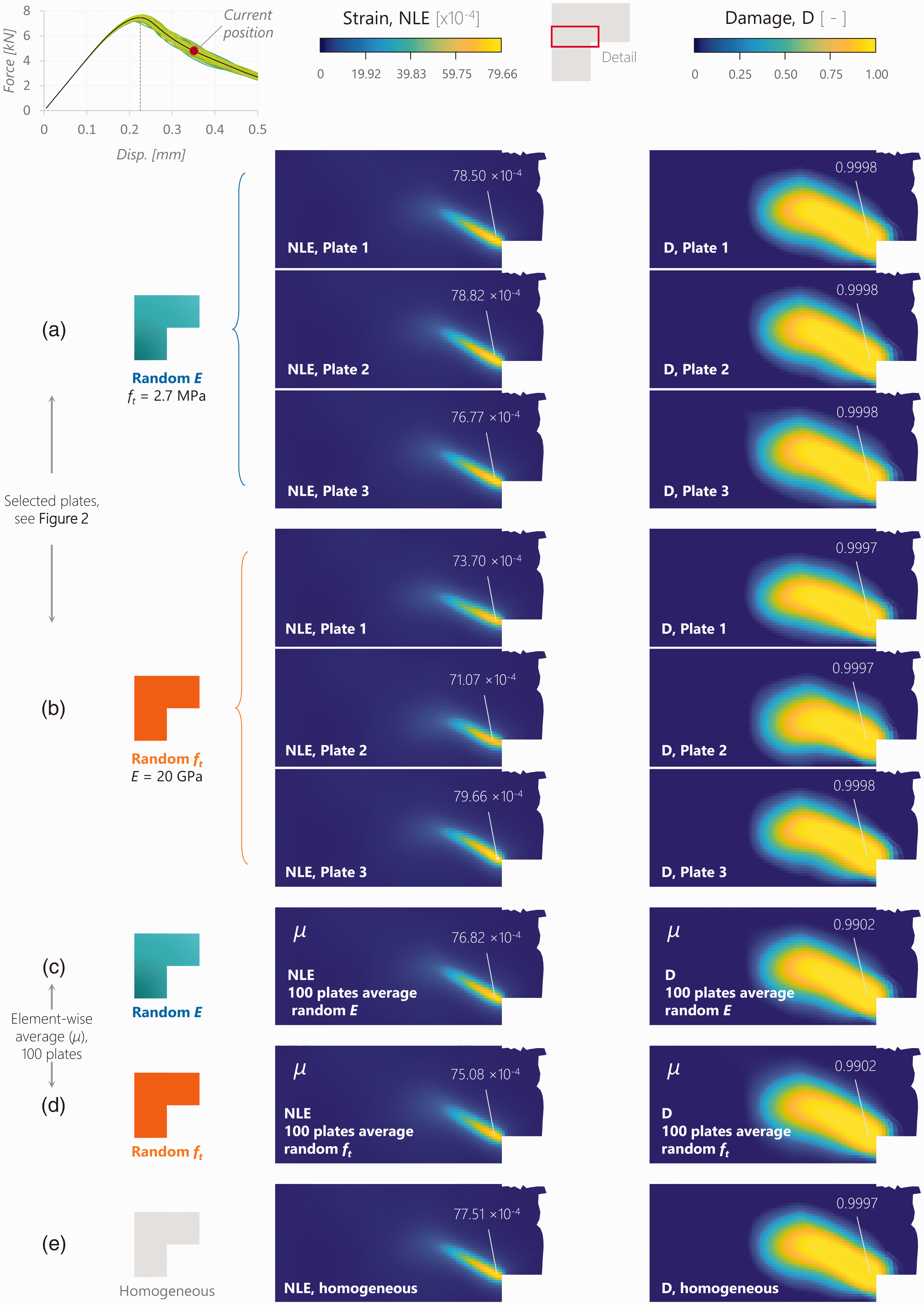
Maps of non-local equivalent strain NLE, and damage D for the L-shaped geometry (detail). The current displacement is presented on the force-displacement curve, top left. (a) Selected random-E specimens, same from Figure 2. (b) Selected random-ft specimens, same from Figure 2. (c) Element-wise average (μ) for 100 random-E specimens and (d) 100 random-ft specimens. (e) Homogeneous specimen. Maximum values are marked. Deformation factor is 0.
We can first contrast the homogeneous results with some of the selected random specimens. The same specimens from Figure 2, i.e. plates 1, 2 and 3 were selected for Figures 7 and 8. In the homogeneous holed specimen (Figure 7(e)), strain and damage concentrate along a horizontal line besides the inclusion; the maps of values are almost completely symmetric. Observing the random-E specimens (Figure 7(a)) some slight asymmetries start to be noticed. While the maps look quite similar, all the element values of NLE and D differ from the homogeneous results, because the underlying E and ft values are random (see Figure 2). For example, the maximum values are unique and now appear distinctively to one or the other side of the inclusion. As it was the case with the previous F-D results, the Young’s modulus appears to have a relatively lower contribution to overall variability.
On the other hand, differences in the strain and damage configurations are much more noticeable in the random-ft specimens (Figure 7(b)). Here, characteristic values such as maxima differ considerably from the homogeneous (and from their counterpart on the other side of the inclusion). The highly strained and damaged areas, or failure paths, are not necessarily horizontal, nor do they have the same general direction at both sides of the inclusion. This ability to ‘wander’ is due to the modeling of spatial variability in the properties of concrete. While unique and different, the values of strain and damage of the random specimens still remain within the same order of magnitude of the homogeneous results.
Similar results were obtained for the L-shaped specimens (Figure 8), where the failure path extends diagonally upwards, away from the inner corner. Overall, the failure paths presented random maxima and inclination; again, variability was lesser for the random-E specimens. Given the larger scale of the L-shaped geometry and its boundary conditions, the associated strains reached a magnitude about five times greater than those of the holed geometry; holed specimens reached slightly lower overall values of damage. The difference in scale between the size of the geometries, as well as the boundary conditions specific to each geometry, can be appreciated in Figure 1. To see the differences among the individual random specimens more clearly it is better to plot NLE and D profiles (see Failure paths section).
Maps of element wise average (μ) and standard deviation (σ) NLE and D
A useful way to summarize the results of the many random specimens that compose each set is to average NLE and D responses of the 100 random specimens, element by element. This generates a corresponding element wise map (μ) of averaged responses (holed geometry Figure 7(c) and (d); L-shaped geometry Figure 8(c) and (d)). Such a map presents a summary of the essential characteristics of the strain/damage maps of the 100 random specimens.
The homogeneous specimens were assigned the same average Young’s modulus and tensile strength than the random specimens. Therefore, the homogeneous and average maps of NLE/D are similar for both configurations. This similarity (1) highlights the consistency of the methodology, which “tends” towards the traditional homogeneous results, and (2) validates that the number of random realizations used in this study is reasonable. Perhaps the most important observation from these maps is that the maxima for NLE and D was lower for the random specimens than for the homogeneous. Maxima of the random specimens was in average ∼1% lower for damage, and for strains it was ∼3% lower (random-ft) and ∼1% lower (random-E). This behavior is analogous to that of peak forces (see Force-displacement curves section).
Perhaps more interesting is the element wise map of standard deviation (σ). The corresponding element-wise standard deviation maps of NLE and D are presented in Figure 9 and Figure 10 for the holed and L-shaped geometries respectively, at four displacement steps. In a homogeneous holed domain (Figure 9) there is little uncertainty that the strains and subsequent damage will initiate at the side “ends” of the inclusion and propagate horizontally. The σ fields offer additional information; in the random specimens, there is a range of elements around the inclusion where critical strain concentrations may potentially lead to failure initiation, depending on the spatial configuration of the properties. Thus, particularly for the random- ft specimens, strain and damage do not initiate always in the same element/location. Meanwhile, failure initiation in the L-shaped geometry is highly localized due to the shape of the domain (Figure 10).
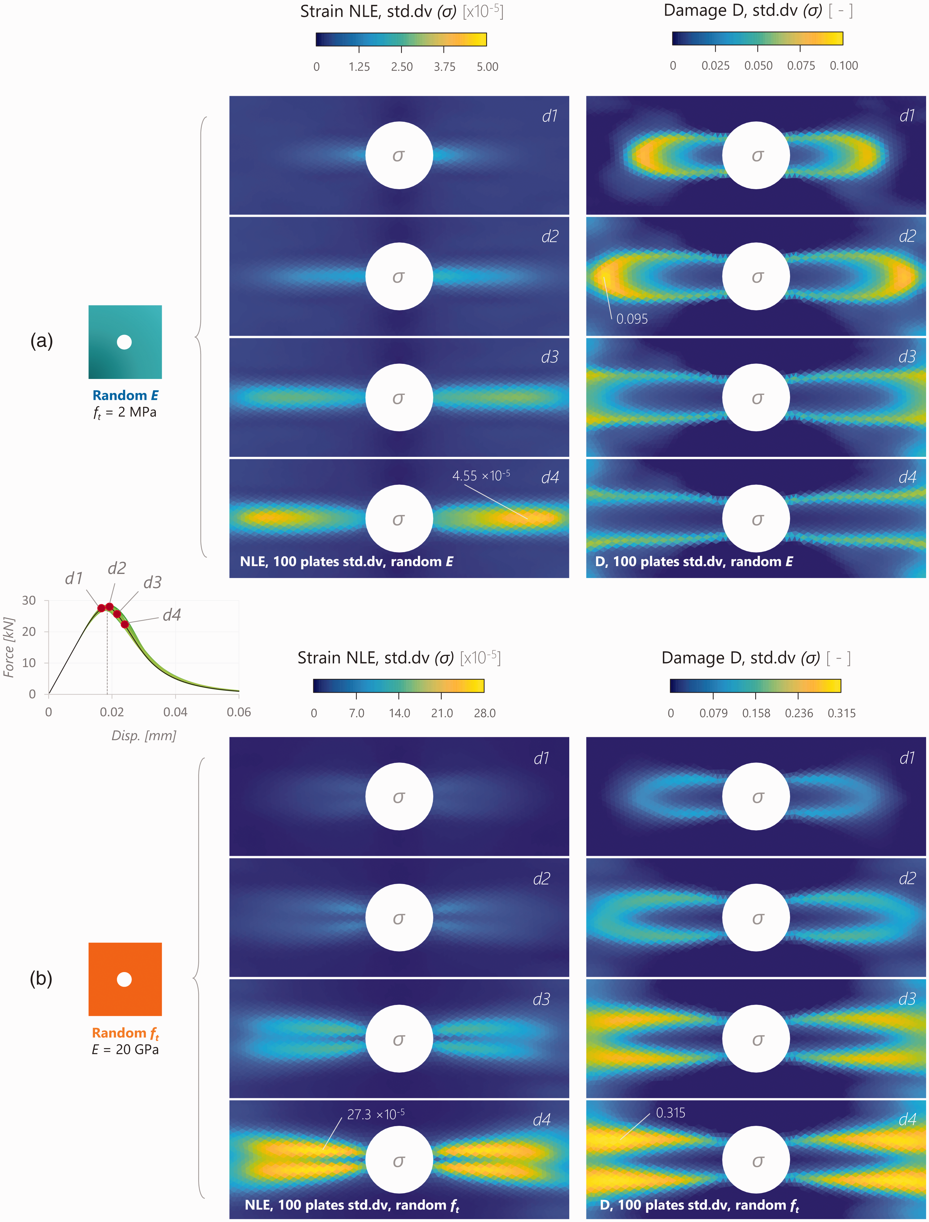
Maps of element-wise standard deviation (σ) of non-local equivalent strain NLE and damage D for the holed geometry (detail). (a) 100 random-E specimens and (b) 100 random-ft specimens. The associated displacements are presented in the force-displacement curve.
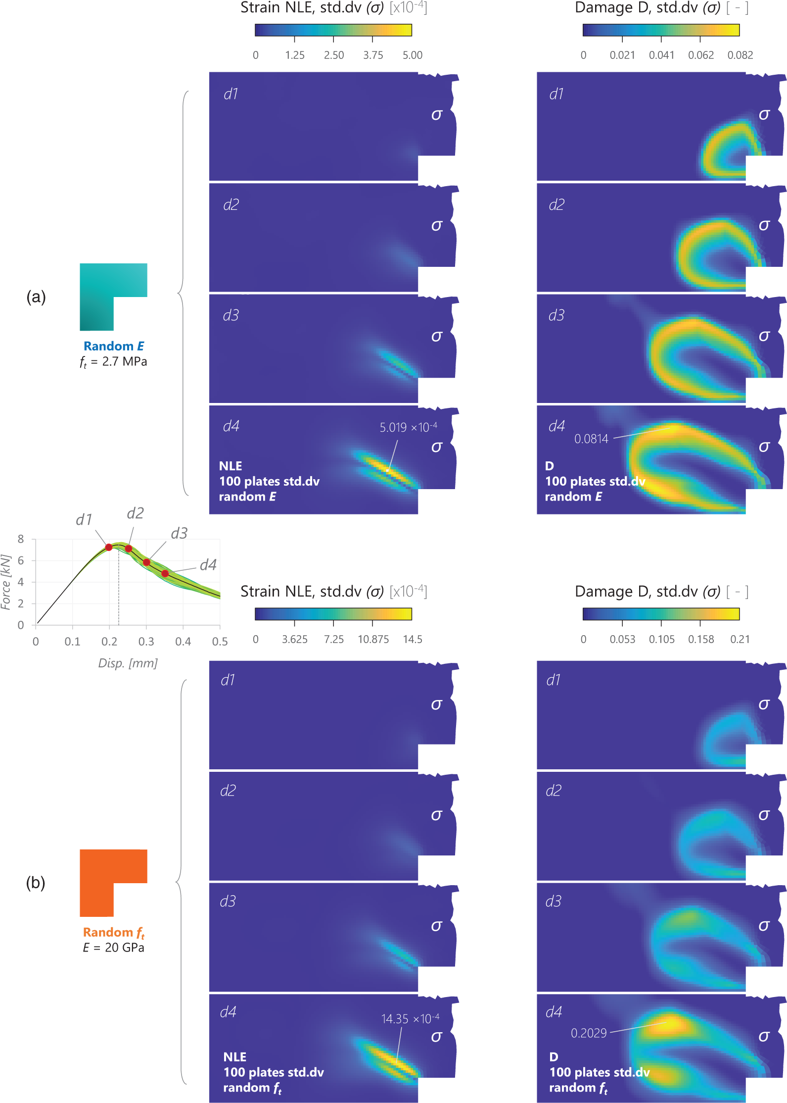
Maps of element-wise standard deviation (σ) of non-local equivalent strain NLE and damage D for the L-shaped geometry (detail). (a) 100 random-E specimens and (b) 100 random-ft specimens. The associated displacements are presented in the force-displacement curve.
While the areas of high concentrations of strains and damage develop and propagate on the specimens, i.e. the failure paths observed in the average (μ) maps, they are surrounded by areas of high uncertainty in strains and damage. These areas of high uncertainty are thinner and more concentrated for the strains than for the damage; except for the random-E holed specimens, strains are “cornered” between two straight paths of high uncertainty. Damage is surrounded by a well-defined “front” of high uncertainty which advances as the displacement is applied. Overall, during the fracture propagation, areas of high uncertainty have a greater extension for damage than for strains. Also, areas of high uncertainty in strains do not correspond with areas of high uncertainty in damage.
As seen before, variability was considerably higher when only ft was random; the maximum standard deviation for damage and strain was 3-5 times higher (holed geometry) and 2.5–3 times higher (L-shaped geometry) for random- ft than random-E. The peak standard deviations of the strains were 5–10 times higher for the L-shaped than for the holed specimens. On the other hand, the standard deviation of damage had similar peak values for the holed- and L-shaped specimens (values were higher for the holed geometry), suggesting that the processes of damage development may have similar levels of uncertainty among these two geometries.
Failure paths
To better examine, summarize and quantify the behavior of the failure paths, they were isolated from each of the random specimens. Failure paths were defined by connecting the nodes with maximum strain (NLE) at each displacement step; the paths coincide for the maxima of NLE and D. The isolated failure paths corresponding to all specimens, along with the values of NLE and D along each path, are presented in Figure 11 (holed geometry) and Figure 12 (L-shaped geometry).
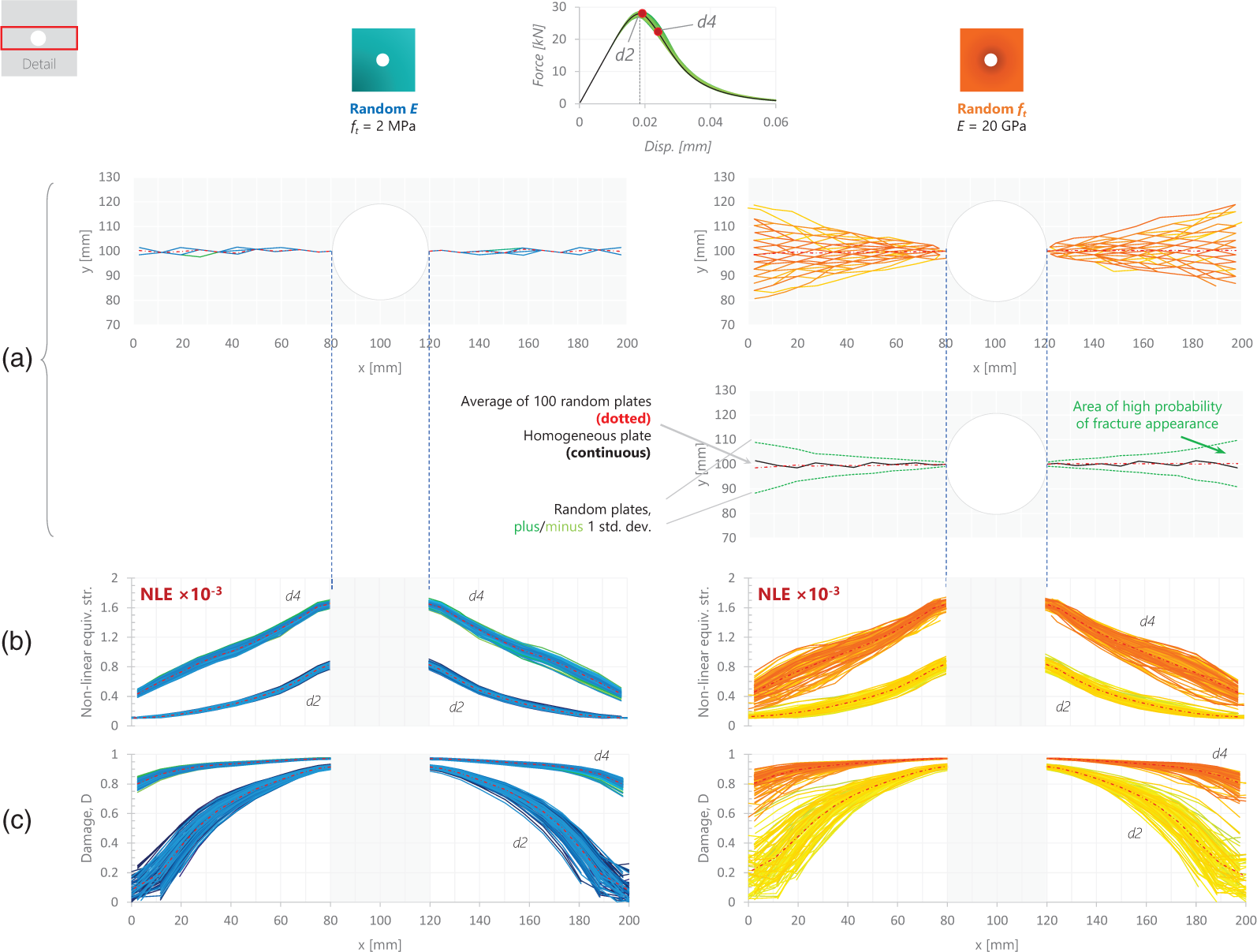
(a) Failure paths of the holed geometry. Failure paths are plotted individually and with a range of ±1 standard deviation. (b) Strain NLE, and (c) damage D, along the failure paths. NLE and D are plotted at two displacement steps, shown in the force-displacement curve.
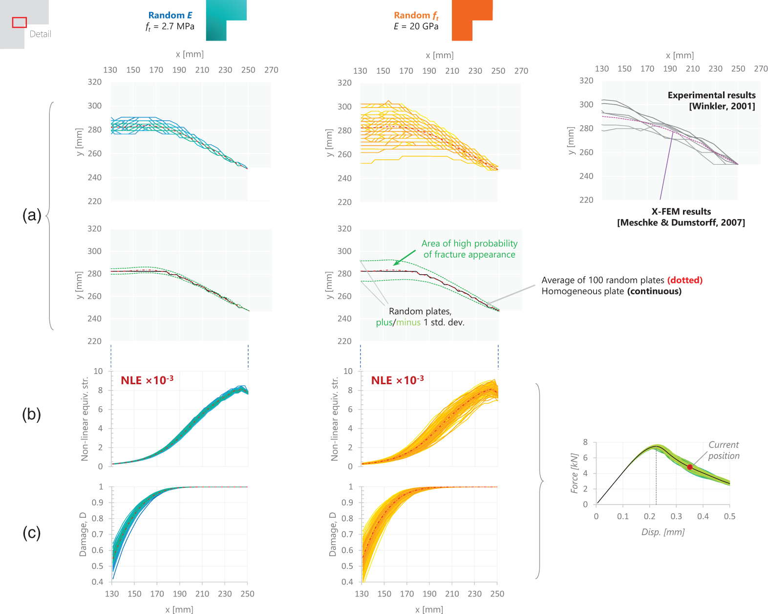
(a) Failure paths of the L-shaped geometry. Failure paths are plotted individually and with a range of ±1 standard deviation. Right-hand side, reported experimental results (Winkler, 2001), front and back of three plates combined, and X-FEM (Meschke and Dumstorff, 2007). (b) Strain NLE, and (c) damage D, along the failure paths. NLE and D are plotted at the displacement step shown in the force-displacement curve.
It was noted before that the random-E specimens showed little variability; this was also the case for the fracture in the holed geometry. While the random-E failure paths (Figure 11(a)) do show some variability, they are mainly straight and deviate little from the horizontal. However, in the random-ft specimens, the failure paths wandered away from their initial location, following random directions and zigzagging outwards. Path orientations were approximately normal, and they deviate around ±10° from the horizontal; they are centered around the path described by the homogeneous specimen. Their general orientation was independent to the left and to the right side of the inclusion. As shown by the NLE and D profiles (Figure 11(b) and (c)), even with low wandering of the fracture, strain and damage are effectively variable along the failure path, particularly toward the outer edges of the specimen.
For the random- ft specimens, the average location of the failure paths is presented along their standard deviation in the vertical coordinate (Figure 11(a)). The plus/minus curves describe a “trumpet” shape within which fracture was most likely to occur. Conceivably, the variability selected to describe the concrete properties could be correlated to different ranges spanned by these curves. While the mesh itself is not coarse, it was not completely horizontal so as not to bias the development of fracture. Therefore, the homogeneous failure path presents a slight but noticeable undulation due to the mesh (continuous line). Interestingly, the average path from the random specimens is almost straight; i.e. a smooth failure path was calculated from the average of the random specimens. This path is closer to the theoretical than that from the homogeneous specimen. Due to the averaging of several specimens, the methodology of random, spatially variable material properties can overcome mesh-related limitations.
Similar observations can be extracted from the L-shaped specimens (Figure 12); slightly more variability was observed here when only the modulus was random, but again ft contributed considerably more to overall variability. The orientation of the failure path in the L-shaped specimens varied from 10° to 15° (random E), and this range increased to 5° to 20° (random ft), effectively describing an area of high probability of fracture around the homogeneous path. Average fracture paths are again smoother than the homogeneous path, and they coincide for random-E and random-ft. The results were compared with fracture paths of L-shaped concrete specimens (Winkler, 2001) and X-FEM results (Meschke and Dumstorff, 2007) (Figure 12(a), right-hand side); the paths described by the computational random specimens are in line with the real fracture paths. Results from the computational model are seen to adjust adequately and represent reasonably well the wandering, shape, and overall orientation of real fracture in specimens of concrete. As stated previously, the force-displacement profiles also compare well (see Figure 6). Additionally, the average-random results for both geometries are comparable with the homogeneous response. The random results are distributed “around” the homogeneous case, which supports their validity.
Summary and closing remarks
Overall summary, main comments
In this paper, we used a methodology to assign spatially correlated random values of Young’s modulus (E) and tensile strength (ft) to specimens of concrete, thus introducing randomness and spatial variability to the computational model. Two geometries were modeled (holed and L-shaped), as well as two types of linear finite elements (triangular and quadrilateral), and two loading schemes (edge displacement for the holed geometry, node displacement for the L-shaped geometry) inducing two different failure modes. The results of the simulations suggest, consistently, that spatial variability of ft contributes more than E to the overall variability of concrete performance in terms of overall force-displacement, strain, damage, and fracture.
Straightforward differences appeared in the strain and damage configurations of the random specimens. Contrary to a homogeneous specimen, randomness in the spatial distribution of material properties leaded to strain, damage and fracture/failure in wandering and uncertain paths, with differing values and location of maxima. Perhaps most importantly, the results from the random L-shaped specimens were comparable and reasonably within the ranges of reported experimental results. This suggests that the model presented in this study is useful for representing and modeling uncertainty-related performance of concrete and other quasi-brittle materials. We believe this also adds validity to the results for the holed plate specimens, as well as to the parameters that were selected herein for modeling the concrete.
Specific conclusions
Tensile strength (ft) contributed greatly to overall variability in performance. Among others, ft contribution to the variability of peak forces sustained by the concrete specimens was 2–3 times greater than that of E alone, and it was 1.7–2 times greater for the associated displacements. In spatial terms, the maximum standard deviation of the strain (NLE) and the damage (D) in the specimens was 3-5 times higher (holed geometry) and 2.5–3 times higher (L-shaped geometry) for random-ft than random-E. ft variability increased the span of potential fracture orientation relative to E variability. In holed specimens, the increase went from 0 (horizontal fracture, random E) to ±10° (random ft), and in L-shaped specimens from 10–15° (random E) to 5–20° (random ft). The associated area of high probability of failure widened accordingly. Fracture wandering was mostly affected by ft variability, although E variability by itself was able to contribute to some extent to wandering depending on the loading configuration. The random specimens were more likely to sustain a lower peak force than a corresponding homogeneous specimen; random specimens therefore predicted an increased probability of failure. These results suggest that considering heterogeneity and randomness may favor the appearance of critical cases for concentration and development of strain and damage in the material. Areas of high uncertainty of strains (NLE) and damage (D) did not have coincident locations. It was found that damage was uncertain over a greater area than the strains, and that areas where uncertainty was high for strains were smaller and closer to the failure path than the areas of high uncertainty of damage. The random failure paths were gathered and used to define areas of high probability for failure occurrence. These areas lie within one standard deviation (in space) from the average response. The variability of E and ft may be correlated proportionally with the width of these areas. In turn, the average failure path coincides with that of the homogeneous response. It was found that the holed configuration may be slightly more sensitive than the L-shaped configuration to the variability of ft. No correlation was found between the maximum force sustained by a specimen, and the maximum-to-minimum value of E or ft occurring on that specimen.
Closing remarks
The methodology is versatile and especially well-suited to assess the individual contribution of parameters to fracture variability. Potentially, more variables could be studied such as the correlation length, length scale, damage parameters, and fracture energy. The parameters relevant to fracture can also be modeled as random in pairs (i.e. E and ft random at the same time), with or without correlation. However, such modeling would limit the possibility of isolating the contribution of the parameters to variability.
In general, the selection of the model parameter values (including standard deviation and correlation length) could be seen as an iterative process to represent the material of interest. At first, representative values should be selected from existing literature and experience. After analyzing the results, the values can be adjusted depending on the response relative to the experimental data. For example, herein it is expected that higher standard deviation (of E, of ft) would lead to greater spread and wandering of fracture; this has been the case after some preliminary testing, as well as for higher length scales. In this way it is also possible to identify parameters that are not contributing significantly to variability.
It is of great interest to engineers and practitioners to understand and gain insight into the spatial variability of the properties of concrete, since it will affect and restrict the adequate performance of the structures. The results of this study show that the methodology can be potentially applied to a variety of domain geometries, sizes, element types, and loading schemes. Features like the management of uneven spatial distribution of mechanical properties, the ability to overcome restrictions imposed by the mesh, and the consideration of extreme and unique propensities to failure, are the kind of modeling considerations that make this modeling methodology powerful, i.e. it is able to go beyond what can be considered in a laboratory setting. Additionally, the methodology presented herein offers an alternative to give insight and complement (expensive) laboratory results, with (relatively inexpensive) computational models; this was one of the motivations of pursuing computational analyses as presented herein.
Another mechanism that could be potentially modeled using this approach is bridging. Bridging refers to agents such as fibers opposing the opening of cracks (Le et al., 2019). Bridging can be modeled implicitly in the continuum damage approach employed in this article. Such a phenomenon may be caused by aggregates as well (Simon and Chandra Kishen, 2016). Parameters such as fracture energy and nonlocal interaction are responsible to control these effects. Being stochastic, these values would represent the uneven distribution of i.e. fibers along the cement paste. Modeling of fracture in domains with inclusions is also a relevant problem in rock fracture mechanics (Janiszewski et al., 2019).
The development of damage in hydraulic concrete, a quasi-brittle material, is a relevant and current issue in infrastructure research. In this context, the results reported herein represent an advance in the study and consideration of the significant role of spatial variability in damage/fracture processes in concrete. None of the previous information would be available from an analysis that included only homogeneous specimens. Fracture processes are random in nature, and while traditional representations of homogeneous materials are useful, greater knowledge can only be attained by introducing randomness into the analysis.
Footnotes
Acknowledgements
The authors appreciate the agreement between SAGE and FinELib, that enabled open-access publication. FinELib is a consortium of Finnish universities, research institutions and public libraries.
Declaration of conflicting interests
The author(s) declared no potential conflicts of interest with respect to the research, authorship, and/or publication of this article.
Funding
The author(s) received no financial support for the research, authorship, and/or publication of this article.