
Abstract
In this study, transfer learning was applied to a Long Short-Term Memory Autoencoder for the detection of rail anomalies across diverse operational conditions. Separate models were trained initially on Laser Doppler Vibrometer data collected from two distinct sites: the Transportation Technology Center in Pueblo, Colorado, and a BNSF railway in Cleburne, Texas. Each site was characterized by unique environmental setups and train speeds (e.g., 10 mph, 20 mph, 30 mph). A cross-dataset evaluation was performed, testing each model on data excluded from its training. Accuracy was observed to decrease in these evaluations, particularly when speed differences exceeded 10 mph or experimental setups differed. Transfer learning was then implemented, retraining portions of the pre-trained models with the new datasets. The results showed that performance has significantly improved after the implementation of transfer learning. It indicates that transfer learning is essential for ensuring accuracy and adaptability across varying conditions for practical applications.
Introduction
Railroads play a vital role in the safety, prosperity, and well-being of our communities and businesses. However, due to increases in train speeds and axle loads that are being applied to aging and deteriorating railroad tracks, the anomaly detection in rail tracks has become of increasing concern for owners and regulators. Current inspection methods, including ultrasonic testing (UT) (Coccia et al., 2009; Mariani et al., 2013; Rose et al., 2003) and eddy current testing (Anandika and Lundberg, 2022; Magel, 2011), have limitations in speed, coverage, and detection accuracy. For instance, UT requires fluid-coupled transducers to examine discrete rail cross-sections, which limit efficiency and real-time defect detection. To address these challenges, non-contact methods based on laser Doppler vibrometer (LDV) measurements have been proposed as promising solutions for rail inspection (Kaynardag et al., 2020, 2022, 2023; Yang, 2023; Yang et al., 2024; Zeng et al., 2024). LDV technology enables high-speed, non-intrusive detection of both surface and subsurface defects, improving the effectiveness of track monitoring (Yang et al., 2023b, 2025). However, LDV measurements are susceptible to uncertainties caused by environmental conditions, track vibrations, and surface variations, which can impact the reliability of anomaly detection.
Machine learning-based tools, such as Support Vector Machines (Li et al., 2021; Liu et al., 2021) Neural Networks (Lu et al., 2020; Mittal and Rao, 2017; Phusakulkajorn et al., 2022) and random forest (Santur et al., 2016), have been proposed to address uncertainty in sensor measurements and improve anomaly detection accuracy for rail inspections. Among these techniques, Long Short-Term Memory autoencoders (LSTM AE) have proven particularly effective for analyzing time-series data, such as that collected from laser Doppler vibrometer measurements. Although computationally more intensive than traditional methods, this trade-off is justified by their superior ability to model sequential data, which is critical for reliability in safety-critical applications. LSTM networks, a specialized form of recurrent neural networks (RNN), are designed to capture long-range dependencies and temporal patterns in sequential data. When implemented as an autoencoder, LSTM models learn a compressed representation of the input sequence and attempt to reconstruct it. Under normal conditions, the reconstructed sequence closely matches the original input, whereas anomalies introduce significant reconstruction errors, signaling potential defects (Verleysen et al., 2015). Despite their effectiveness, training robust LSTM AE models for real-world applications can be challenging, particularly due to the variability in operational conditions (e.g., train speeds, track types, and sensor configurations) (Shafiq et al., 2022; Tien et al., 2021; Yehezkel et al., 2021) and the limited availability of labeled data. Although the precise moments when LDVs passed over anomalies were recorded, the duration of each defect’s influence on the time-domain signal remained unclear, and labeled data distinguishing normal from abnormal conditions were absent. Despite this uncertainty about anomaly duration, identifying specific time segments free of anomalies was considered essential for viable training data. The lack of precise labeling complicated the analysis and application of machine learning techniques, highlighting the need for adaptive strategies. To overcome these challenges, transfer learning has been investigated to enhance model adaptability by utilizing knowledge from previously trained models. This technique involves freezing certain pre-trained layers while retraining others with new datasets, proving effective in improving rail damage detection performance (S. X. Chen et al., 2021; Gibert et al., 2015; Xie et al., 2023; Zheng et al., 2021).
In this study, the application of transfer learning was explored to improve rail defect detection using LDV measurements. Field tests were conducted in Pueblo, Colorado, and Cleburne, Texas, where a rail car equipped with two LDVs recorded railhead vibrations induced by rail-wheel interaction forces at three different speeds: 16 km/h (10 mph), 32 km/h (20 mph), and 48 km/h (30 mph). The recorded LDV signals were first filtered to eliminate impulsive noise (Kaynardag et al., 2025), and then the filtered signals were used to train an LSTM autoencoder model for anomaly detection. Given the data was recorded under different operational conditions, a cross-dataset evaluation was first conducted to test the model’s robustness when applied to different datasets (Y. Chen et al., n.d.). This comprehensive analysis consisted of two primary evaluations: (i) assessing the model’s accuracy in detecting rail anomalies across various operational speeds, and (ii) evaluating the model’s consistency across different experimental setups. Based on the cross-dataset evaluation results, transfer learning was implemented in the LSTM Autoencoder model by freezing certain layers’ weights and retraining others for the new dataset. It was observed that transfer learning was essential when the model, trained on data with a speed difference exceeding 10 mph compared to the testing data. Similarly, for different experimental setups, applying transfer learning to the initially trained model was necessary to ensure its adaptability under varied conditions. This study provides valuable insights into the application of transfer learning with LSTM Autoencoders for rail inspection, contributing to ongoing efforts in enhancing rail safety. This paper is organized as follows: Data collection and pre-processing Section describes the data collection process during the field tests, and the corresponding data preprocessing algorithms. LSTM Autoencoder Section provides an overview of the LSTM AE model architecture. Cross-dataset evaluation Section focuses on cross-dataset evaluation and the implementation of transfer learning. The results and their implications are discussed in Results Section, and the paper concludes with future recommendations presented in Conclusions Section.
Data collection and pre-processing
In this research, datasets from two distinct field tests were used to train the model and implement transfer learning. The first test was conducted on a rail track with one welded joint at the High Tonnage Loop (HTL) at the Transportation Technology Center (TTC) in Pueblo, Colorado. The second test was carried out on a BNSF railway track in Cleburne, Texas. Both sites featured 136 lb. (61.68 kg) A.R.E.A (The American Railway Engineering Association) rails with various rail anomalies. Data were recorded by LDV at multiple train speeds. After the data collection, the impulsive noise filter was first applied to the raw LDV data, then several data-preprocessing techniques were implemented to signal features, including feature extraction, correlation analysis, log transformation, standardization, and principal component analysis.
Field tests at TTC
The first field test, conducted on the High Tonnage Loop (HTL) at the TTC in Pueblo, Colorado, consisted of a ballasted railway track, fasteners (e-clip), and wooden ties. The rail span was approximately 0.5 meters long. It was anchored to the ties via steel baseplates and elastic rail clips. In this setting, a welded joint was strategically incorporated to simulate both the reflected and transmitted waves induced by the rail anomalies (Long and Loveday, 2014; Loveday et al., 2020; Loveday and Long, 2015). The test involved mounting two Laser Doppler Vibrometers (LDVs) on a rail car, which then travelled over the track segment with the welded joint at three different speeds: 16km/h (10mph), 32 km/h (20mph) and 48 km/h (30mph), capturing rail head vibrations due to wheel-rail interaction forces. This system uses LDV measurements to detect a change in the relative amplitudes of the recorded waves caused by a defect. An overview of the experimental setup is shown in Figure 1.
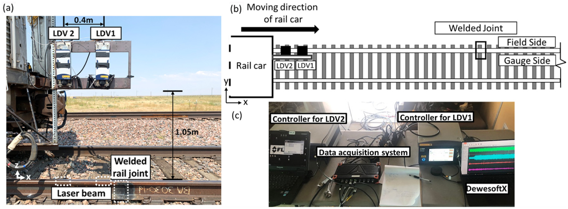
Field tests at TTC: (a) Damage detection system mounted on the rail car (b) the schematic view of the damage detection system, inspected rail track and the anomaly, and (c) the set-up inside the rail car with two controllers and the data acquisition system.
Two different LDV systems were used: a single-beam Polytec Vibroflex Xtra MLV-I-120 and a tri-beam Polytec MLV100 Xtra. To mitigate vibrations affecting the LDVs during motion, eight vibration isolators (Soitec MP28-58I) were placed at the corners of each LDV, and then attached to a steel frame. The lift-off distance was set as 1.05 meters and laser head separation was chosen to be 0.4 meter in a preliminary study. Inside the rail car, controllers for the LDVs and a Dewesoft Sirius-XHS data acquisition system were set up to record the signals. The system used a sampling frequency of 1.25 MHz to reduce noise and refine the signal within the targeted frequency range.
Field test in Cleburne, TX
The second field test was carried out at the railway track in Cleburne, Texas. This railway track was operated and maintained by Burlington Northern Santa Fe (BNSF) Railway Company. The ballasted railway track consists of spikes and wood ties. In contrast to the first field test’s-controlled environment, the second field provided a more complex and real-world environment. The vibration data was recorded through the two LDVs mounted on the rail car as shown in Figure 2 (a). The configuration for the second field test utilized a 0.5-meter distance between the LDVs and a 0.97-meter lift-off distance, differing from the setup used in the first field test. In this field test, the two LDVs mounted on the rail car are the same. Both LDVs were tri-beam Polytec MLV100 Xtra. The controllers for the LDVs were placed inside the equipment box shown in the Figure 2 (b) along with data acquisition system (Dewesoft Sirius-XHS) and a back-up power bank. A sampling frequency of 1.25 MHz was maintained, with vibration isolators minimizing noise during motion.
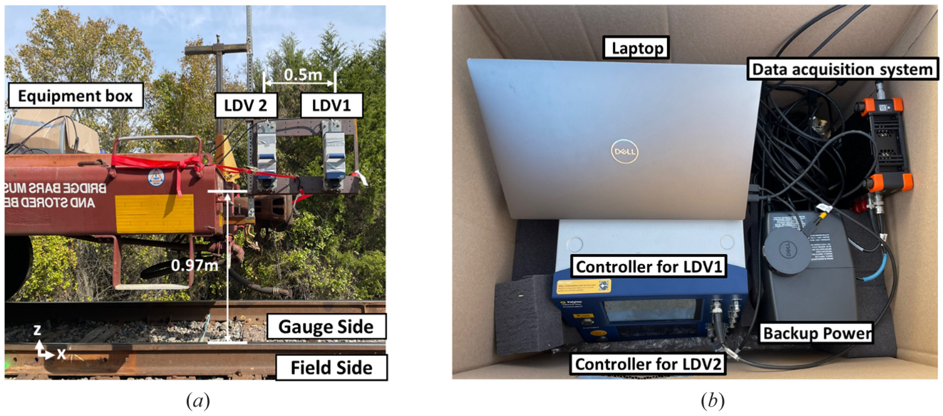
Field tests in Cleburne, TX: (a) Damage detection system mounted on the rail car at the second field test (b) the set-up inside the rail car with two controllers and the data acquisition system.
Compared to the track conditions in the first field test at TTC, the track environment in the second field test presented a higher level of complexity. This increased complexity was presented by a greater number and variety of defects observed along the track as shown in Figure 3 (a). In the second field test, two types of anomalies were marked along the rail: (i) transverse defect (TD) with steel reinforcement segment (see Figure 3 (b) and Figure 3 (c), and (ii) welded joint as shown in Figure 3 (d). To detect these anomalies through moving measurements, the LDVs were mounted on the rail car and running pass through the rail at two different speeds: 16 km/h (10 mph), 32 km/h (20mph). These two field tests allowed for a thorough investigation of rail anomaly detection algorithms under varying operational conditions. It provides a deeper understanding of the performance evaluation of the ML models trained for anomaly detection.
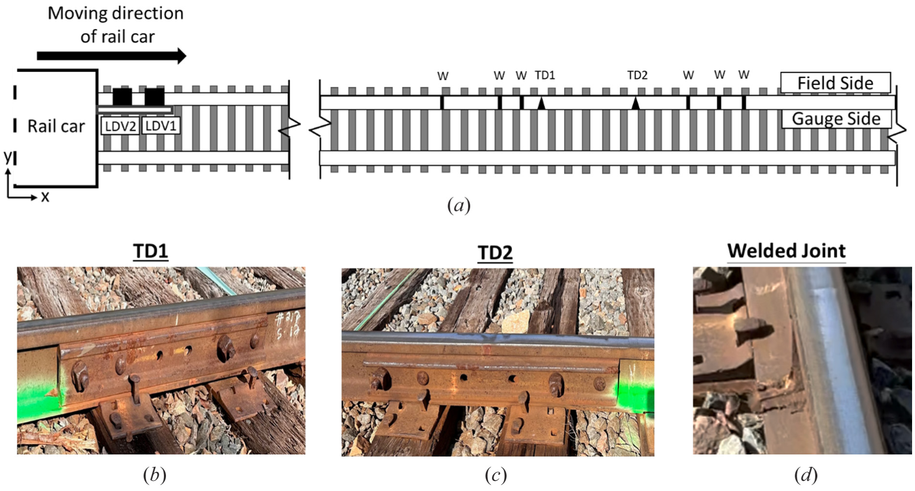
(a) The schematic view of the damage detection system, inspected rail track and the anomalies, (b) the first transverse defect, (c) the second transverse defect and (d) the welded joint.
Data preprocessing
A data processing procedure was implemented to prepare the LDV data for the training of the LSTM AE models. The flowchart of the procedure is shown in Figure 4, and consists of five steps: (1) impulsive noise filtering, (2) feature extraction, (3) correlation analysis, (4) log transformation and standardization, and (5) principal component analysis.
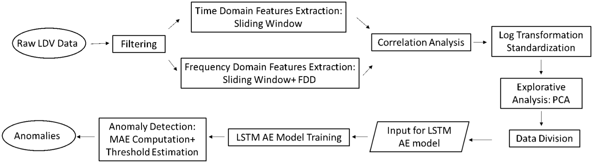
Flowchart of data preprocessing.
First, the impulsive noise filtering was implemented on the raw LDV data. The LDV signal typically exhibits a fluctuating non-zero mean and is susceptible to impulsive noise (IN). These effects become intensified during the moving measurements. Addressing this issue is critical to ensure the machine learning model’s accuracy. A moving average filter was first employed to eliminate the time-varying non-zero mean from the LDV signal (Su et al., 2015). Next, an impulsive noise filter developed in a preliminary study (Kaynardag et al., 2025), was implemented to reduce the impact of IN on the collected data. The impulsive noise filter consists of two key steps: (i) detection, identifying segments of the signal that contain IN, and (ii) estimation, which estimates IN-free values by replacing those segments. To effectively mitigate IN, the filter targets two types of contaminants, which are artificial peaks and artificial fluctuations. During the detection phase, the Hampel Identifier, a robust outlier detection method, was utilized to identify artificial peaks [31], while the Stationary Wavelet Packet Transformation (SWPT) method was used to locate artificial fluctuations. In the estimation phase, an algorithm based on constrained least squares replaced segments with artificial peaks, while a moving average filter with Gaussian weights was used to substitute segments with artificial fluctuations. Consequently, this comprehensive filtering process significantly mitigated the influence of impulsive noise on the LDV data.
After the LDV data was filtered, several steps were taken to prepare the data for the model training, including feature extraction (Appendix A1), correlation analysis (Appendix A2), log transformation and standardization (Appendix A3), and principal component analysis (Appendix A4). These steps collectively transform time-domain LDV signals into a format suitable for LSTM AE machine learning models. Six signal features, including the standard deviation, Kurtosis, Shannon Entropy, Shape Factor, Spectrum Root Mean Square and Signal Energy were extracted and used to train the LSTM AE models for different operational conditions.
3. LSTM Autoencoder
In this study, a Long Short-Term Memory Autoencoder (LSTM-AE) model was developed to detect rail anomalies using multivariate time series data. The LSTM-AE integrates the LSTM network, designed for sequential data processing, with an Autoencoder architecture designed to compress and reconstruct the input data. The LSTM network features memory cells and gates, such as the input, forget, and output gates. These gates regulate the information flow based on current and past data, employing sigmoid activation functions to determine what data to retain or discard (Staudemeyer and Morris, 2019). This structure allows LSTM to preserve relevant information and filter out irrelevant details, effectively capturing the temporal dependencies in the data.
The Autoencoder component includes an input layer, encoder, latent representation, decoder, and output layer (Tschannen et al., 2018), as shown in Figure 5. The encoder is structured to transform the input data (
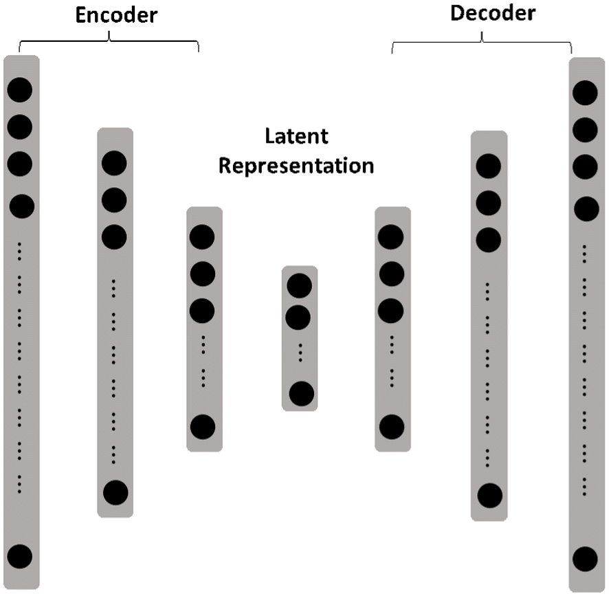
The architecture of an Autoencoder.
To examine the data flow in the LSTM-AE neural network, the pipeline is analyzed using sample data, as illustrated in Figure 6. The dataset consists of
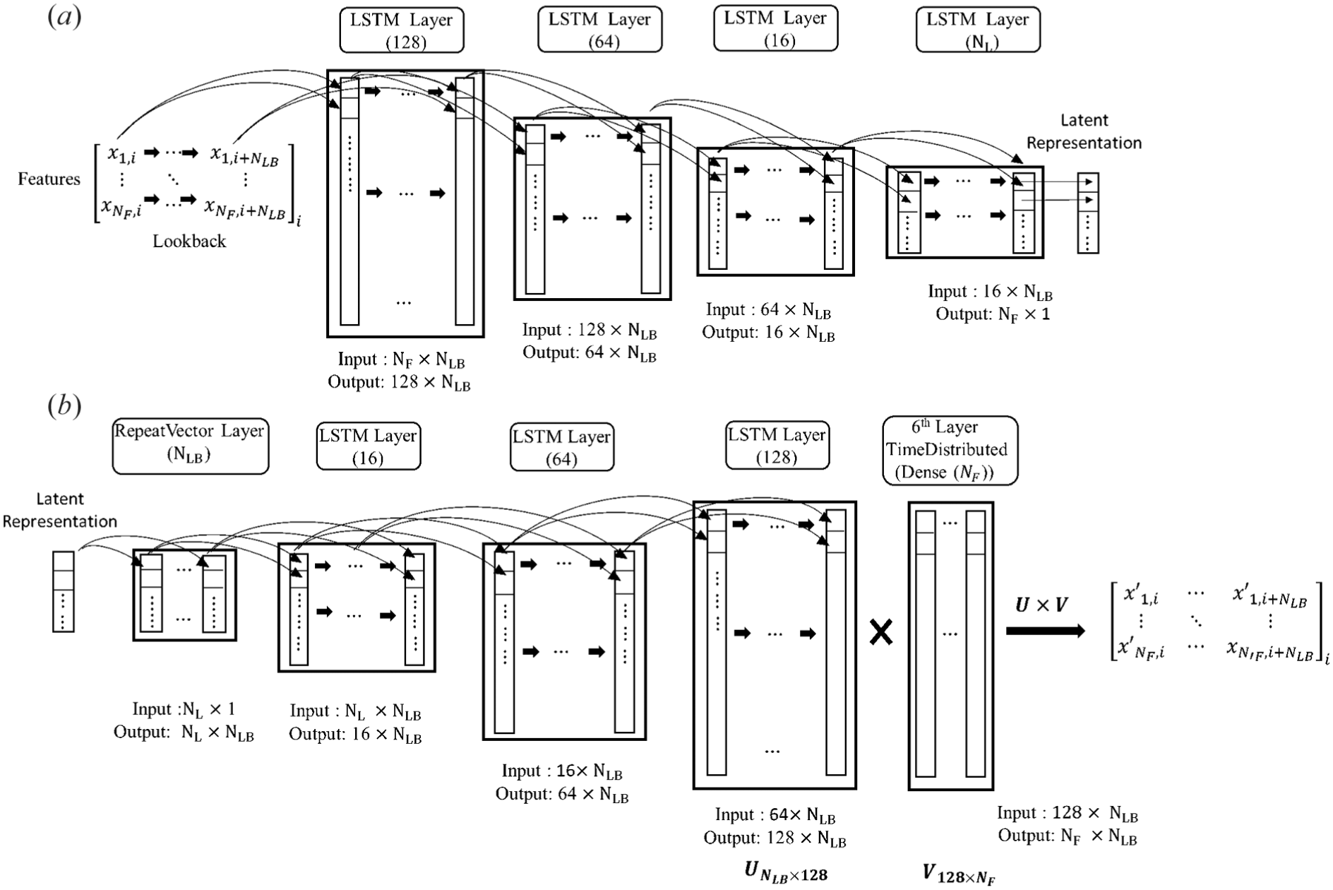
Architectural diagram of the LSTM autoencoder: (a) encoder structure compressing the sequential input features into a low-dimensional latent representation; and (b) decoder structure reconstructing the original sequence from the latent space representation.
Anomaly detection
To conduct anomaly detection in this study, it is necessary to calculate the reconstruction error and establish a threshold first. The reconstruction error represents the discrepancy between the input signal and its reconstructed output signal. This error (denoted as
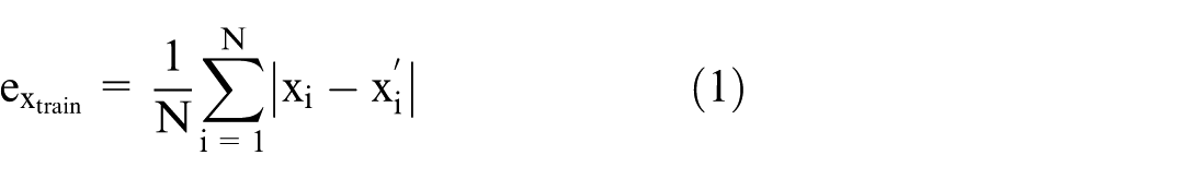
Here,

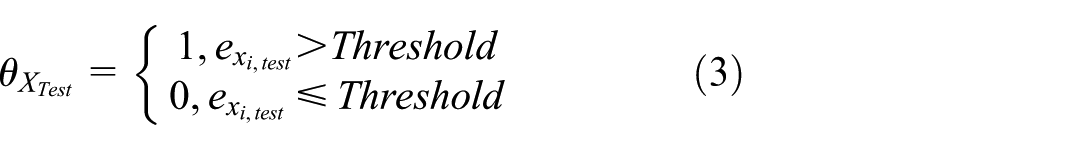
A test data point (
Cross-dataset evaluation
In this study, cross-dataset evaluation was conducted to test the adaptability and robustness of a model trained on one dataset when applied to others. This analysis was divided into two parts: (1) The first part focused on assessing the model’s ability to detect rail anomalies across different train speeds. (2) The second part examined the model’s performance across varying experimental setups.
Cross-dataset evaluation for different speeds from the same set-up
In this section, cross-dataset evaluation was performed using data collected from field tests at the Transportation Technology Center. The dataset collected from multiple speeds was used to assess how speed variations affect the model’s performance in detecting rail anomalies. Two speed differences were examined: a moderate difference of 16 km/h (10 mph) and a larger difference of 32 km/h (20 mph). For instance, the 16 km/h difference was evaluated by training the model on data collected at 16 km/h and testing it with data from 32 km/h. It results in a 16 km/h speed gap between training and testing sets. The performance of anomaly detection at a 16 km/h (10 mph) speed difference is presented in Figure 7. The gray areas in the time series highlight the detected anomalies, while dashed lines indicate the approximated time instants when the LDVs passed the anomalies. Figure 7(a) shows results for the LSTM-AE model trained on 16 km/h data and tested on 32 km/h data. Conversely, Figure 7(b) shows the performance of the model trained on data from a 32 km/h environment when tested against data from a 16 km/h setting.
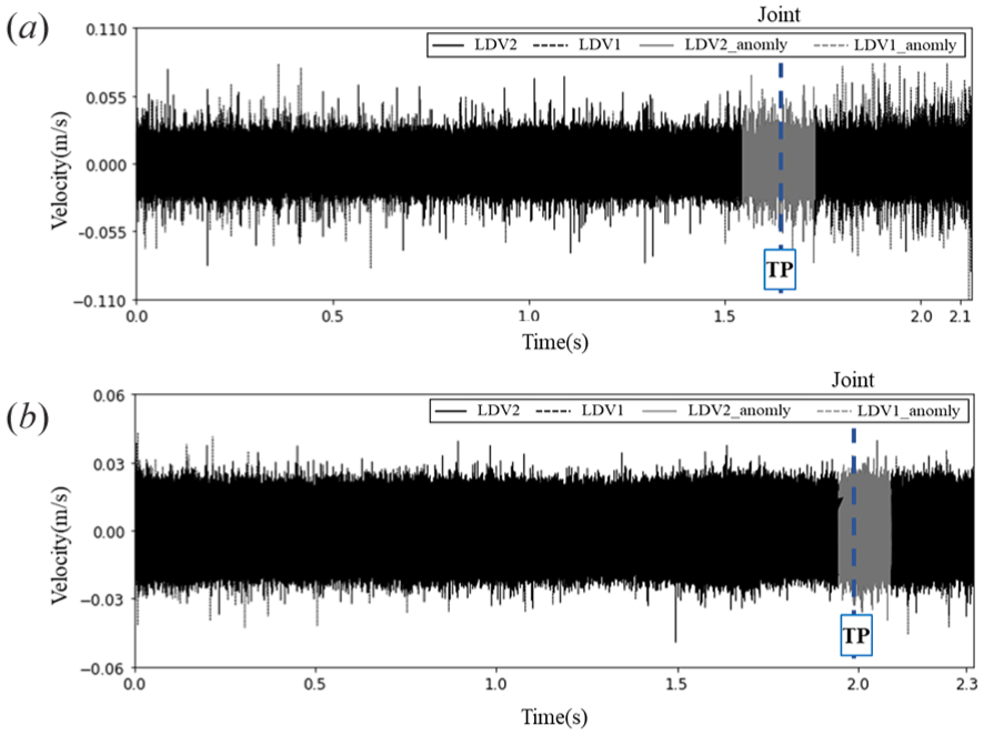
Cross-dataset evaluation: 16km/h (10mph) difference, anomaly detection results of (a) model trained using data collected at 16 km/h to test on data collected at 32km/h, and (b) Model trained using data collected at 32 km/h to test on data collected at 16km/h.
To evaluate the model’s performance, an event-based approach was adopted. The ground truth consists of known defect locations recorded as discrete time instants, while the model identifies an anomaly over a continuous segment of time where the reconstruction error exceeds the threshold. Therefore, the following criteria were used for classifying the outcomes shown in the figures: (i) A True Positive (TP) is recorded if a model-detected anomalous segment overlaps with a known ground-truth defect instant. (ii) A False Positive (FP) is recorded if a detected anomalous segment does not correspond to any known defect location. (iii) A False Negative (FN) is recorded if no anomalous segment is detected by the model at a known ground-truth defect location. A True Negative (TN) represents the segments where no defect was present and none was detected, are omitted for simplicity.
The consistency in successful anomaly detection across these speed variations suggests the model’s robustness to moderate speed changes (16km/h or 10mph). However, the analysis becomes more complex at a 32 km/h (20 mph) speed difference, as shown in Figure 8. Figure 8 (a) reveals certain challenges, such as an increase in false positives (i.e., where no defect is present, but the model identifies one), when the model trained on 16 km/h data was tested on 48 km/h data. It indicates a possible reduction in detection accuracy under larger speed gaps. Similarly, Figure 8 (b) reveals similar false detections when the model trained on 48 km/h data was evaluated against 16 km/h data. Despite these challenges, the model retains its core ability to identify key anomalies, though with limitations due to significant speed differences between training and testing datasets. These findings suggest that, for datasets collected at speeds differing by 32 km/h (20 mph) or more from the training data, applying transfer learning techniques could adjust the model to new conditions, maintaining its accuracy and reliability.
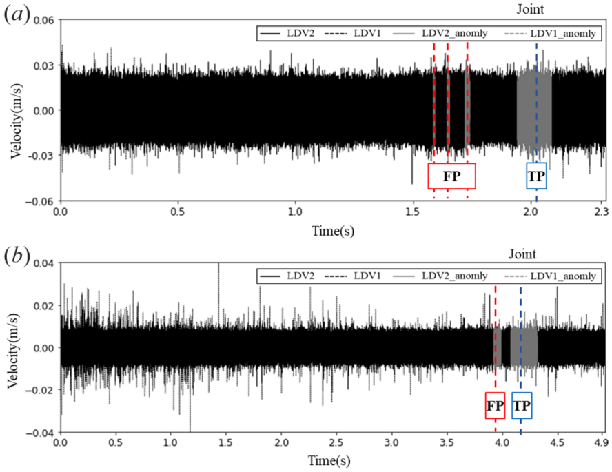
Cross-dataset evaluation: 32km/h (20mph) difference, anomaly detection results of (a) model trained using data collected at 16 km/h to test on data collected at 48km/h, and (b) Model trained using data collected at 48 km/h to test on data collected at 16km/h.
Evaluation across distinct experimental configurations with constant velocity
In this section, datasets from a subsequent field test (see Section: Field Test in Cleburne, TX) were used to assess the model’s generalization across different experimental setups while maintaining a constant train speed. The second dataset was collected under rail conditions that were substantially more complex than those in the first field test. It thereby imposes challenges on the development of the rail anomaly detection algorithm. Both the training and the evaluative datasets were collected at a uniform speed of 20 mph to eliminate speed as a variable. Results of this cross-dataset evaluation are shown in Figure 9. A bar above the time series indicates the locations of different defect types: TD1 for transverse defect 1, TD2 for transverse defect 2, and W for welded joint (see section 2.2). The pre-trained model exhibits a notable increase in false positives (FP), alongside instances of false negatives (FN) and true positives (TP), as observed in the time series data; true negatives (TN) are omitted for simplicity.
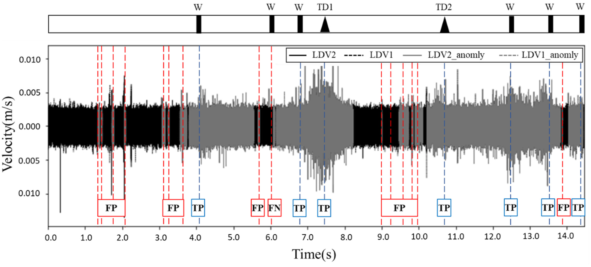
Anomaly detection results from the cross-setup evaluation, showing the performance of the model trained on the TTC dataset when tested on the BNSF dataset.
These errors, particularly the high rate of false positives, reduce the reliability of the LSTM-AE model under complex conditions. In order to overcome this limitation, the adoption of transfer learning techniques is proposed as a potential solution, allowing the model to be adjusted to the specific characteristics of the data from the second field test.
Transfer learning
In this study, transfer learning was applied to an LSTM autoencoder for rail anomaly detection. It improves the model’s adaptability to varying operational speeds and different experimental setups. This approach is particularly useful when new experimental data is limited or expensive to obtain, as it allows the model to leverage knowledge from previously learned tasks. The process reuses parts of the pre-trained model and fine-tunes them with a smaller dataset collected under new conditions, such as a different speed or setup. Figure 10 shows the flow chart of the transfer learning methodology adopted in the study.
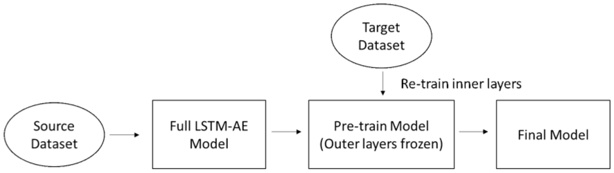
Flowchart of the transfer learning methodology.
The strategy for fine-tuning involves selectively retraining certain layers while keeping others frozen, a choice guided by the hierarchical nature of feature learning in deep networks (Tien et al., 2021). The initial layers of an encoder typically learn general, low-level features that are broadly applicable across different conditions. The middle layers, however, capture more abstract, task-specific representations that are most sensitive to changes in operational conditions. Therefore, by freezing the initial layers and retraining the middle layers, the model can efficiently adapt to the new domain while retaining its fundamental knowledge. This method conserves resources by avoiding the need to train a model from scratch and reduces the amount of data required for high accuracy.
In this study, transfer learning was implemented to retrain the middle five layers of the model, as shown in Figure 11. The first two layers in the encoder and the last three layers in the decoder were frozen. Specifically, in the encoder, the 3rd, and the 4th LSTM layer (which contains 16 and 3 hidden layers, respectively) were retrained using the new dataset. The latent space and the initial layers of the decoder (containing 3 and 16 hidden layers) were also retrained to adapt the model to the new data characteristics. Consequently, the neural network components critical for capturing characteristics related to the new speed or setup were updated.
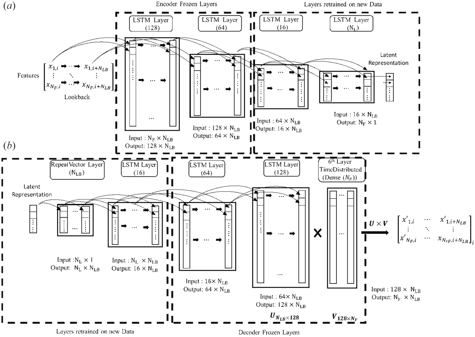
Architectural diagram of the LSTM autoencoder for transfer learning: (a) encoder showing the frozen lower layers and retrained middle layers used to adapt the model to new data; and (b) decoder highlighting the corresponding retrained initial layers and frozen output layers involved in reconstructing the input sequence.
This targeted retraining requires less data points and less effort to train the model since it builds upon prior knowledge learnt from previous datasets. Additionally, a lower learning rate is helpful to fine-tune the middle layers without drastically changing the characteristics captured in the previous training stage. While a learning rate of 0.01 was used in the initial training, a rate of 0.001 was used during the transfer learning stage to fine-tune the inner layers.
Results
In this section, the results of anomaly detection employing transfer learning are presented. Initially, the application of transfer learning for cross-dataset evaluation across various speeds within the same experimental setup is illustrated in Figures 12 and 13. Figure 12 shows outcomes from a model pre-trained with data at 16 km/h and enhanced through transfer learning with data collected at 48 km/h (30 mph). The evaluation of the model also utilized data from the 48 km/h speed. Figure 12(a) shows the Mean Absolute Error obtained after applying transfer learning, alongside the established threshold. A data point is classified as an anomaly if its reconstructed MAE loss exceeds this threshold. The detection results, combined with LDV time series data, are shown in Figure 12(b). Compared to results before transfer learning (See Figure 8), the LSTM Autoencoder model’s performance has improved significantly, now detecting anomalies accurately without false positives.
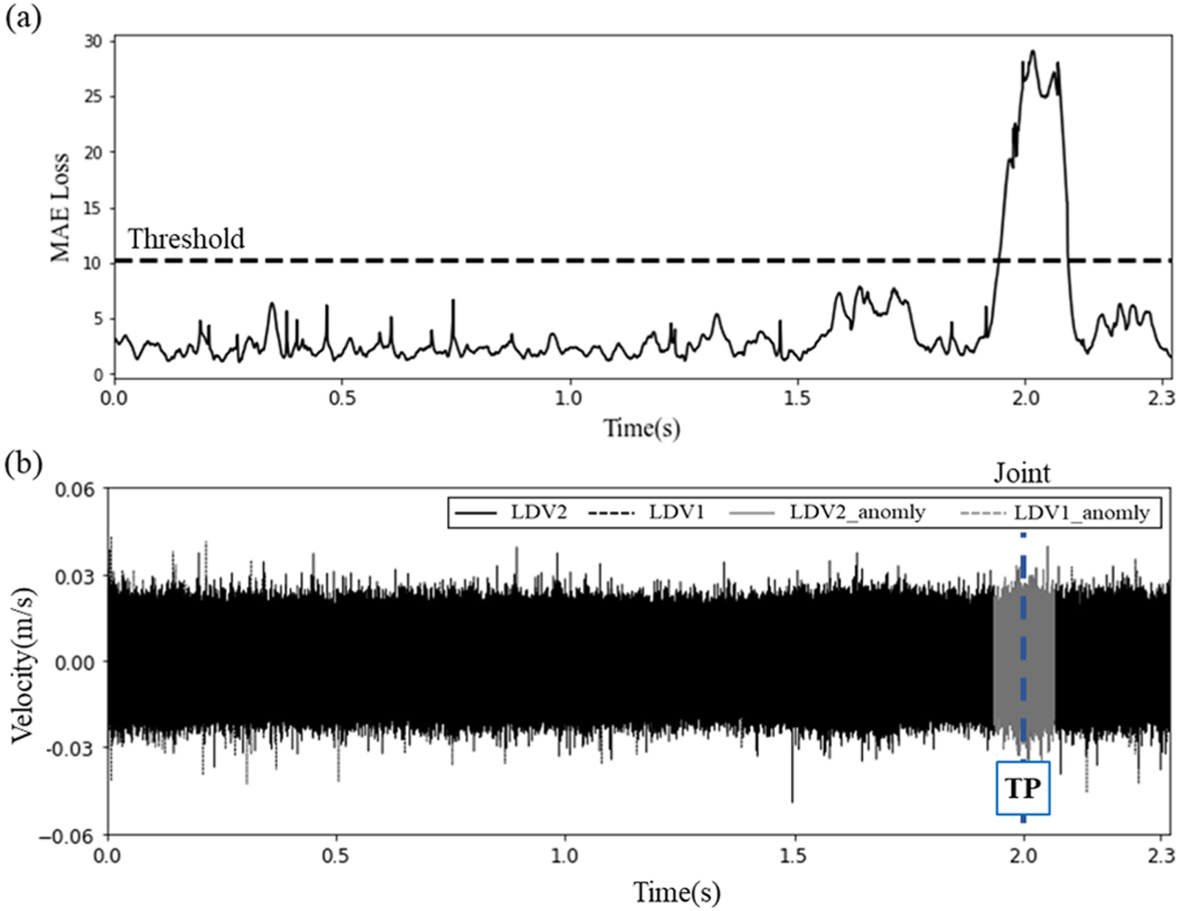
Anomaly detection results of the model pre-train using the data collected at 16km/h and transfer learning from the data collected at 48 km/h (30mph), and evaluated the model with the data collected at 48 km/h. (a) The MAE loss and (b) the detected anomalies in the LDVs time series data.
Anomaly detection results of the model pre-train using the data collected at 48km/h and transfer learning from the data collected at 16 km/h, and evaluated the model with the data collected at 16 km/h. (a) The MAE loss and (b) the detected anomalies in the LDVs time series data.
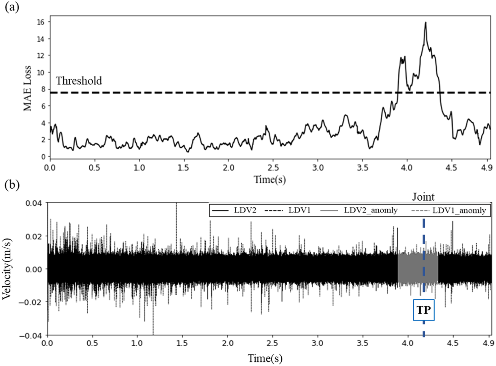
Similarly, Figure 13 presents the results obtained from the model pre-trained with data collected at 48 km/h (30 mph) and adjusted via transfer learning with data from 16 km/h (10 mph). The model’s evaluation was then conducted with data collected at 16 km/h. Figure 13 (a) shows the MAE after transfer learning and the corresponding threshold. Figure 13 (b) shows the anomaly detection outcomes alongside LDV data. Compared to the cross-dataset evaluation shown in Figure 8, these results demonstrate that transfer learning enables a model trained at one speed to adapt effectively to another, highlighting its robustness across varying operational conditions.
Next, the results from the model pre-trained with data collected at TTC and adapted through transfer learning with data collected from BNSF at 32 km/h are shown in Figure 14. The corresponding event-based metrics are presented in Table 1. As the table demonstrates, applying transfer learning significantly improved the model’s performance in this cross-setup evaluation. Precision saw a dramatic increase from 33.3% to 87.5%, a change driven by the reduction of false positives from 14 to just 1. While the recall remained the same, the substantial gain in precision led to a much higher and more balanced F1-Score, which increased from 48.2% to 87.5%. This quantitatively proves that transfer learning made the model more reliable and less prone to false alarms.
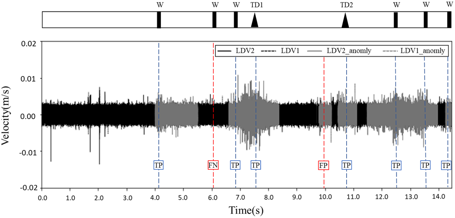
Anomaly detection results of the model pre-train using the data collected at TTC and transfer learning from the data collected with BNSF.
Event-based performance metrics before and after applying transfer learning for the cross-setup evaluation.
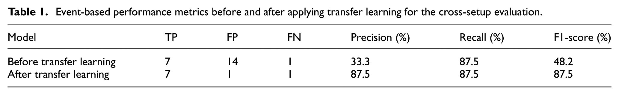
The remaining false positive and false negative may be attributed to the greater complexity of the second field test, as the track conditions at Cleburne are much more intricate than those at the TTC test farm. This suggests that detecting rail defects in real-world scenarios may require a more sophisticated model and precise defect documentation. Consequently, the findings indicate that when the model was trained on data with a speed difference exceeding 10 mph from the testing data, transfer learning is essential for improving accuracy. Similarly, for different experimental setups, applying transfer learning to the pre-trained model is recommended to ensure adaptability and precision under varying conditions.
Conclusions
In this study, transfer learning was applied to an unsupervised machine learning approach developed based on laser Doppler vibrometer measurements for rail anomalies detection. The vibrational data of the rail was collected at varying train speeds from two distinct sites with unique environmental conditions and experimental setups: the Transportation Technology Center in Pueblo, Colorado, and a site in Cleburne, Texas. After data collection, filtering and signal processing was implemented to extract key features in both time and frequency domains. This was followed by correlation analysis, log transformation, standardization, and Principal Component Analysis to prepare the input data for training and validating. LSTM Autoencoder models were trained separately using datasets from these diverse speeds and set-ups. Next, a cross-dataset evaluation was conducted, illustrating the importance of transfer learning in improving the model’s performance across varied conditions. It was observed that when training data exhibited a speed difference exceeding 10 mph from testing data, transfer learning was essential for a robust model. Similarly, for different experimental setups, applying transfer learning to the initially trained model is strongly recommended.
In both instances, whether addressing speed discrepancies or differing experimental conditions, transfer learning proved critical in refining the model’s performance. By adopting transfer learning, the model’s ability to accurately respond to diverse datasets was markedly improved.
For future work, several avenues could be explored to build upon this research. In the current tests, the time instant when the damage detection system passed the rail anomalies were recorded manually, therefore a more precise approach, such as Global Positioning System and high-speed camera may be necessary to improve the validation accuracy of the model. Also, even though the field tests involve more than one type of rail defect, the model implemented is unable to classify them. To address various damage scenarios (e.g., wearing, corrugation, gauge widening, transverse defect, etc.), the development of a more sophisticated machine learning model is suggested. To further refine the current transfer learning strategy, a comparative study could perform a sensitivity analysis on the fine-tuning process by exploring the impact of freezing or retraining different layers to optimize the model’s performance. Finally, this study utilized a feature-engineering methodology where signal features were explicitly calculated; a promising direction would be to investigate end-to-end deep learning models, like 1D-CNNs, that process raw sensor data directly to learn relevant features automatically (Han et al., 2024). This would allow for a more comprehensive understanding of the approach across different railway tracks in service.
Footnotes
Appendix A1. Features extraction
In this study, the feature extraction from time series data was performed by implementing a sliding window method. This method involves moving a window of a fixed size windowing with a time step along the signal. For each position, the values within a sliding window are analyzed to transform the time-series data into a lower-dimensional representation. It reduces computational costs and improves calculation efficiency. Data from two LDVs were initially recorded at a sampling frequency of 1.25 MHz. These signals were then down-sampled to 62.5 kHz. Next, a low-pass filter was applied with a cutoff frequency of 25 kHz (Yang et al., 2023a). For the test speed of 16 km/h (10 mph), a sliding window with a duration of 0.01 seconds and a time step of 0.001 seconds was employed. For a speed of 32 km/h, the window and time step were set at 0.08 seconds and 0.0008 seconds, respectively. At 48 km/h (30 mph), the chosen window size was 0.005 seconds with a time step of 0.0005 seconds. The selection of window sizes balanced several factors: (i) computational time for feature extraction, (ii) the resolution in time and frequency domains, and (iii) ensuring at least 2000 data points for neural network input.
In Structural Health Monitoring, signal features from both time and frequency domains are crucial for damage detection. These features can change as a fault progresses, altering the normal signal pattern (Liu et al., 2021). In this study, separate features were extracted from the two LDV datasets: (i) Time domain features included maximum absolute value (SF1), peak-to-peak value (SF2), standard deviation (SF3), kurtosis (SF4), root mean square (SF5), Shannon’s entropy (SF6), skewness (SF7), crest factor (SF8), and shape factor (SF9), and (ii) Frequency domain features (in the 0–25 kHz range) included spectrum root mean square (SF10) and signal energy (SF11). The specific implementation of signal energy and the relevant frequency range were established in preliminary studies (Yang et al., 2023a, 2024). The signal features used and their corresponding formulas are detailed in Table 2.
In Table 2, the LDV signal from the two LDVs is denoted as
To derive frequency domain features, Frequency Domain Decomposition (FDD) was applied to the LDV signals. FDD, a non-parametric, output-only system identification method, was used to obtain the frequency spectrum (Brincker et al., 2001). For each sliding window, the time domain data were analyzed using FDD to obtain singular values of the time domain signal in the window, denoted as
Eventually, from the readings of each LDV, eleven types of signal features could be extracted. For instance, the SF1 feature from the first LDV was labeled as
Appendix A2. Correlation analysis
Correlation analysis is a widely used method to identify relationships between variables in the data, specifically input features in neural networks. It serves two key purposes: (i) it helps reduce the risk of overfitting by identifying and eliminating features with potential collinearity issues, and (ii) it assists in feature selection for dimension reduction. The analysis produced Pearson’s correlation coefficients, which measure the strength of relationships between feature pairs. The correlation coefficient ranges from −1 to 1. A correlation coefficient close to 1 or −1 indicates a strong relationship between the variables. A coefficient of 1 signifies a perfect positive correlation, while −1 denotes a perfect negative correlation.
Following the extraction of 22 features as described in the previous section, correlation analysis was performed. In this study, features with an absolute correlation coefficient exceeding 0.8 were considered highly correlated. One of these features would then be removed from the input set. An example of correlation analysis results from one of the data sets (data collected at TTC at 32 km/h) is illustrated in Figure 15. In this figure, a highly positive correlation coefficient between two features is represented by a white color, whereas a highly negative correlation is indicated by black. It was observed that the correlation coefficients of features were consistent across different data sets. After the correlation analysis, 12 features were chosen for the next stage of data preprocessing for all data sets:
Appendix A3. Log transformation and standardization
Log transformation is a common technique used to convert skewed data sets into more symmetric, near-normal distributions. In this study, several factors justified the use of log transformation: (i) the distribution of the variables (i.e., features) was normally distributed when measurements were taken on an intact rail, (ii) the feature values were exclusively non-negative and non-zero, and (iii) the application of log transformation led to stable model performance, as evidenced by the training and validation loss in preliminary studies. For this research, any data with a skewness value exceeding 0.75 was classified as skewed. The skewed data underwent log transformation using the following equation:
An example of the distribution of one feature, specifically the Maximum Absolute Value (SF1), before and after log transformation, is depicted in Figure 16. The originally right-skewed distribution shifted toward a normal distribution after log transformation. It helps stabilizing the training of the neural network. Following the log transformation, standardization was applied to rescale the data. This process involved subtracting the mean of each feature from individual data points and dividing by the standard deviation of that feature. After standardization, the data was centered around the mean, with the variance normalized to ensure that the features were on a comparable scale.
Appendix A4. Principal component analysis
Machine learning architectures can become highly complex and computationally intensive when processing high-dimensional data. This complexity often leads to slower training processes and can potentially diminish the model’s performance. To address this, Principal Component Analysis (PCA) is frequently employed for two main purposes: (i) feature extraction, which involves transforming the input features into a lower-dimensional representation (i.e., generated features) while retaining the essential information, and (ii) feature selection, where features are ranked based on their variance contribution, allowing users to prioritize them for in-depth analysis.
In this study, feature selection was utilized to pinpoint the features that most effectively explained variance across various datasets. Through the application of PCA, six features emerged as the most representative and explained a significant portion of the variance compared to others:
Acknowledgements
The authors are grateful to Robert Wilson, the program manager of the FRA, for his technical guidance and valuable comments during all phases of this research. Furthermore, the authors would like to acknowledge the help of Brian Lindeman from TTCI and David Sheperd from BNSF for providing valuable help in performing the field test as well as Vikrant Paklant from Polytec for providing technical support. The authors are thankful to Guan-Wei Lee from the Smart Structural Research Group at UT Austin for helping and providing insight into the initial ML model configuration.
Author note
Any opinions, findings, conclusions, or recommendations expressed are those of the authors and do not necessarily reflect the views of the FRA.
Funding
The authors disclosed receipt of the following financial support for the research, authorship, and/or publication of this article: This work has been supported under the grant number: 693JJ619C000005 awarded by the Federal Railroad Administration of the US Department of Transportation.
Declaration of conflicting interests
The authors declared no potential conflicts of interest with respect to the research, authorship, and/or publication of this article.
Data availability statement
The datasets generated and supporting the findings of this article are obtainable from the corresponding author upon reasonable request.