
Abstract
Civil structures are often overdesigned to meet safety and functionality criteria under rare, strong events. Adaptive structures, however, can modify their response through sensing and actuation to satisfy design criteria more efficiently with better material utilization, which results in lower resource consumption and associated environmental impacts. Adaptation is performed through actuators integrated into the structural layout. Several methods exist for optimal actuator placement to control displacements and internal force flow. In discrete systems like trusses and frames, actuator placement is typically a binary assignment. Most existing methods use bilevel and heuristic formulations, leading to suboptimal solutions without proving global optimality. This paper introduces a Mixed Integer Programming (MIP) method that produces global optimum solutions by optimizing both actuator placement and commands. Two objective functions are used: minimizing the number of actuators and minimizing control energy. The optimization considers structural and serviceability limits and control feasibility. An extensive benchmark compares the new formulation’s global optima with solutions from greedy, stochastic, and heuristic methods. Results show that the new method consistently produces higher-quality solutions than all other methods benchmarked in this study.
Keywords
1. Introduction
1.1. Previous work
Building construction and operation are responsible for a substantial share of global energy consumption, greenhouse gas emissions, and waste generation (United Nations Environment Programme (IEA), 2022). The construction sector is a major consumer of mined raw materials leading to the depletion of resources once believed unlimited (e.g. sand, metals) (United Nations Environment Programme, 2014). The material used for construction causes 9% of the annual global CO2 emissions, and overall the building industry contributes to more than 34% of the global energy demand (United Nations Environment Programme (IEA), 2022). Addressing these challenges requires a change in the way civil structures are designed. Civil structures must satisfy safety and serviceability criteria under strong and rare events and therefore are typically overdesigned for most of their service life. Instead, structures could be adaptive in response to strong but infrequent loads and other environmental actions (Preumont and Kazuto, 2008; Soong and Spencer Jr, 2000; Utku, 1998; Wani et al., 2022). A key aspect that allows adaptive structures to be resource-efficient is the ability to reach a compromise between the stiffness provided through geometry and mass (i.e. element sizing) and the extent of active compensation of stress and displacement responses caused by external actions. Active response mitigation against strong but infrequent loading events enables material, embodied carbon and energy minimization, especially for stiffness-governed configurations such as tall and slender buildings (Blandini et al., 2022; Reksowardojo and Senatore, 2023; Senatore et al., 2018), long-span bridges (Reksowardojo et al., 2024a; Zeller et al., 2023) and floor systems (Nitzlader et al., 2022; Reksowardojo et al., 2024b). In these cases, it is much more efficient to compensate the response under loading actively when needed than embodying additional material, which is a cost penalty for most of the service life of the structure since typical design loads are caused by strong events that occur infrequently (Senatore et al., 2019). Response mitigation under loading can also be employed to increase durability and extend the service by reducing the stress response below relevant fatigue initiation thresholds which is particularly relevant for bridge structures (Canny et al., 2024).
For discrete structural assemblies such as trusses and frames, adaptation can be performed by linear actuators that are integrated into the structural layout. The action of linear actuators, for example, length changes, has been employed to control the response of truss and frame configurations, including high-rise and bridge structures (Abdel-Rohman and Leipholz 1983; Geiger et al., 2020; Rhode-Barbarigos et al., 2010; Rodellar et al., 2002; Wagner et al., 2020). Several actuator placement methods have been formulated to maximize the efficacy of controlling displacements and the internal force flow (Böhm et al., 2019; Lu et al., 1992; Ramesh et al., 1991; Senatore and Reksowardojo, 2020; Steffen et al., 2022). In most previous methods for discrete assemblies, actuator placement has been implemented as a binary (0–1) assignment to element sites. The binary decision variable is typically relaxed by evaluating the effect of a unitary action of candidate actuators on displacement and internal forces, which is collated in sensitivity (i.e. influence) matrices (Du Pasquier and Shea, 2022; Senatore et al., 2019; Steffen et al., 2020). Other approaches including stochastic methods (Du Pasquier and Shea, 2021; Furuya and Haftka, 1995; Yan and Yam, 2002), bilevel approaches (e.g. Stackelberg Game) (Ali et al., 2015; Marker and Bleicher, 2022; Wagner et al., 2018; Zeller et al., 2022) and other sequential formulations (Manguri et al., 2023; Rashid et al., 2022; Saeed et al., 2023; Wani and Tantray, 2022) have been implemented. Typically, these methods produce actuator placements with optimality degrading as the problem dimension increases and constraints are tightened (e.g. displacement limits).
All-In-One (AIO) structure-control optimization methods have been formulated in (Senatore and Wang, 2024; Wang and Senatore, 2020) that can produce global least-weight and minimum energy adaptive structures. In these formulations, variables related to the structural layout (e.g. sizing, topology) and actuator placement are optimized simultaneously. For this reason, using such methods it is not possible to evaluate the effect of certain objective functions and constraints only on the actuator positions and to benchmark solutions with other actuator placement methods. This is particularly important for retrofitting applications; in which cases the structural parameters must be kept constant since the structure is already built. Methods for the optimal retrofitting of multi-story structures that minimize the number of actuators and the control energy that produce global optima have not yet been formulated.
Previous studies (Virgili et al., 2023) do not include benchmarks between solutions produced by sequential and AIO methods. Importantly, no systematic investigation has been carried out in the literature to compare the performance of diverse actuator placement methods against global benchmarks.
1.2. New contribution
The new contributions of this work are:
A method based on Mixed-Integer Programming (MIP) that can optimize simultaneously actuator positions and commands, hereafter referred to as “All-In-One” (AIO) actuator placement. Two objective functions are formulated: (O1) minimize the number of actuators, and (O2) minimize the control energy, both under quasi-static loads. Optimization constraints include structural, serviceability and control feasibility.
New objective and constraint functions specific to the actuator placement problem are provided. The formulation is linear for O1 and quadratic for O2, and therefore in both cases, it can be solved to a global optimum using state-of-the-art branch and bound algorithms.
A proof of the problem convexity to minimize the control energy (O2), which contains bilinear constraint functions.
Rigorous comparison of the performance of diverse methods based on sequential approaches including heuristics, greedy and stochastic strategies against the global benchmarks obtained with the AIO approach.
Benchmarks are carried out in terms of two key performance indicators, namely the number of actuators and the control energy required to satisfy target control objectives that include stress, displacement and actuator force limits.
Section 2 provides the formulation for the structural and control system model. Section 3 outlines different optimal control strategies under equivalent static representations of dynamic loads (e.g. wind). In Section 4, performance metrics are defined to evaluate the quality of the solutions. In Section 4.3.3, a benchmark is carried out between the new AIO formulation and several sequential methods. Case studies on multi-story building structures are employed to evaluate the influence of different input parameters including the number of structural elements and control constraints.
2. System modeling
Pin-jointed structures are considered with the assumption of small deformations and linear elastic material. Under static loads, the system equilibrium is

where

Uncontrolled state: (a) displacements, (b) internal forces; all elements have identical cross-section
The control input matrix
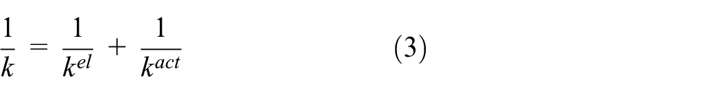
For simplicity, since the actuator stiffness
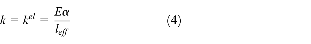
For short truss elements and large cross-sections, the actuator stiffness might affect the serial stiffness and therefore should be considered.
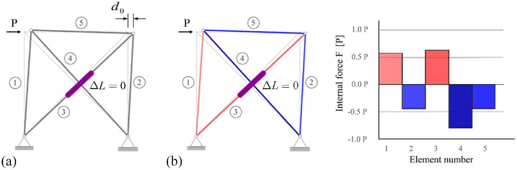
Consider the truss structure in Figure 1, which is equipped with one actuator to reduce the horizontal displacement response under load
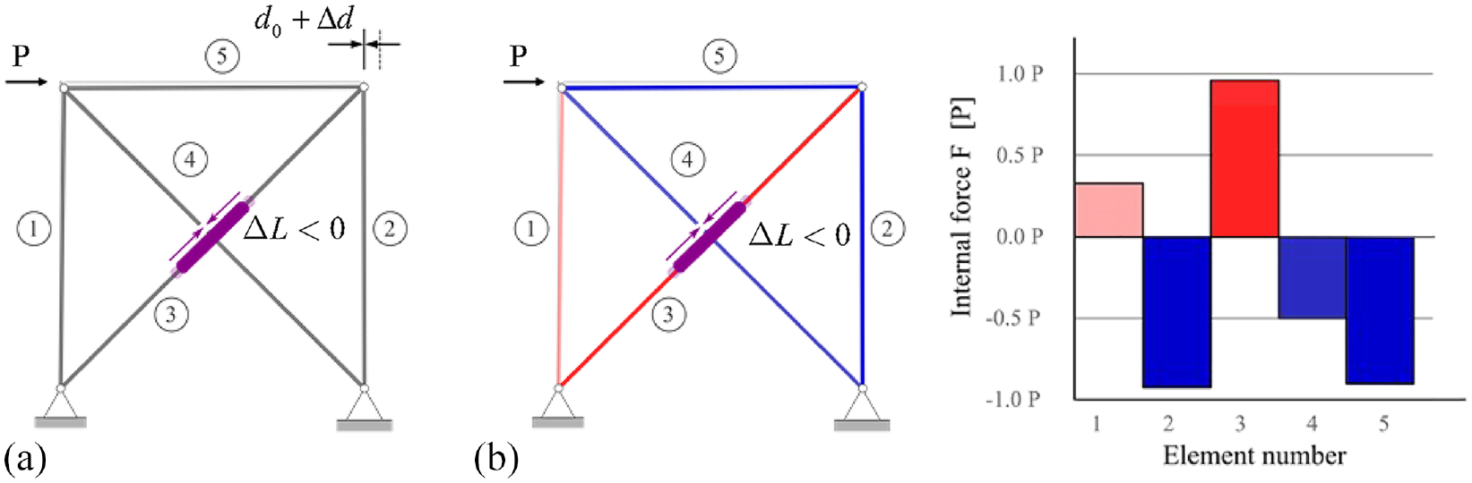
Controlled state with complete compensation of horizontal displacement

where

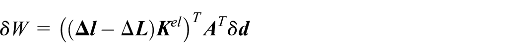
The virtual work due to internal forces

Expressing

Expressing

where

The equivalent actuation load consists of a pair of self-equilibrated forces applied by the active element to the connecting nodes, producing an inelastic displacement
The controlled system is described as

The control input matrix can thus be written as

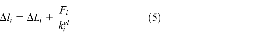
The change of displacement caused by

The internal element force change

In equation (13), the element force is obtained by subtracting from the total deformation
Figures 1(b) and 2(b) show the variation of the internal forces for a negative length change of the actuator positioned in the diagonal element #3 to achieve a complete compensation of the horizontal displacement in the upper nodes (see Figure 2(a)). The effect of actuation to reduce the displacement response can be typically controlled to obtain an overall homogenization by increasing the utilization of elements that are not critically stressed.
For simplicity to achieve a formulation that can produce global optima, the effect of geometric nonlinear has not been considered. The assumption of small strains and displacements has been experimentally validated on several large-scale prototype structures including a 6m span simply supported bridge (Senatore et al., 2017) and a 36 m tall 12-story adaptive tower (Dakova et al., 2024). Geometric non-linearity was accounted for a new method to design structures that adapt to loading through large shape reconfigurations, that is, shape morphing (Reksowardojo et al., 2022; Reksowardojo and Senatore, 2023), which is not considered in this work.
Dynamic effects are only considered in the definition of static-equivalent loading conditions since the focus is on determining effective positions to place linear actuators and not on closed-loop dynamics. For slender and lightweight structures with low vibration periods (T1 > 1 s) and with the principal vibration mode shapes similar to the deformed shape under static loading, controlling the steady-state response is usually the dominant design requirement for the control system. This is the case for slender cantilever structures under lateral loads as the one considered in the case studies in Section 4.3.3. The actuator performance in compensating for static displacements is representative of the upper bound (i.e. largest amplitude) of the dynamic response. In the case of seismic design, equivalent static loads can be determined from the response spectrum, which, for structures meeting regularity criteria, for example, simple geometry with uniform mass and stiffness distribution, is adequate to model the effect of seismic loads (European Committee for Standardization (CEN), 2005).
3. Constrained optimal control
Several strategies have been proposed to achieve optimal response control under static load cases. A formulation proposed in (Wagner et al., 2018), uses a Moore-Penrose pseudo-inverse matrix (Penrose, 1955) to determine the control inputs that yield the minimum L 2 -norm of the displacements for the controlled nodes. In (Böhm et al., 2019) the same approach is proposed to achieve stress homogenization in structural elements. However, these methods do not account for specific load cases nor structural and actuation constraints. In (Senatore and Reksowardojo, 2020), control strategies are formulated based on constrained minimization to obtain optimal control inputs for different targets: (C1) simultaneous displacement and element force control to satisfy strength and serviceability limits; (C2) displacement control without causing a change in element forces (Impotent eigenstrain); (C3) element force without causing a change in displacements (Nilpotent eigenstrain); (C4) displacement control through actuation energy minimization subject to stress and stability constraints.
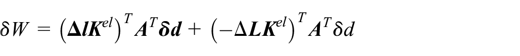
Following (Senatore and Reksowardojo, 2020), in this work, the control problem is formulated through the minimization of the discrepancy between a correction target to satisfy serviceability limits
where


where


where
4. Actuator layout optimization
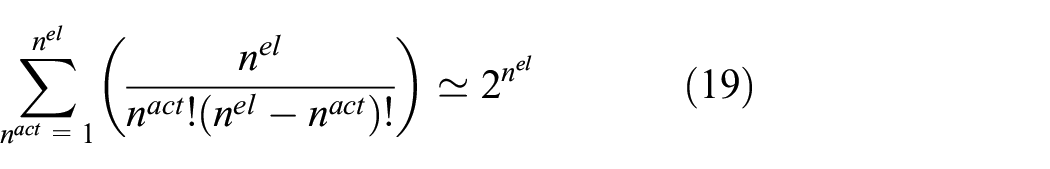
The determination of an efficient actuator set is typically a combinatorial optimization problem that involves selecting a subset from a finite set of possible placements. When all elements are candidate sites for actuators, the number of placements increases exponentially with the number of structural elements
Computation of all possible sets is not feasible, optimal solutions have been obtained through methods involving integer relaxation (Senatore et al., 2019) through efficacy ranking, mixed-integer programming formulations (Senatore and Wang, 2024; Wang and Senatore, 2021), and metaheuristics (Furuya and Haftka, 1995; Zeller et al., 2022).
Minimizing the number of actuators in control system design is important due to cost efficiency, control strategy simplicity, reduced risks of failure, and low maintenance and installation efforts. On the other hand, employing a higher number of actuators allows smoother and more precise control over a wider range of load events. Similarly, limiting the operational energy of the system is important to ensure control feasibility, reduce operational costs, enhance system reliability, and reduce adverse environmental impacts. These two objective functions are inversely correlated: reducing the number of actuators generally requires more energy for the system to satisfy the control targets.
4.1. Performance metrics
Given a truss structure, the assignment of an actuator to an element position
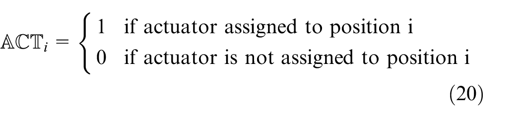
If the ith entry of
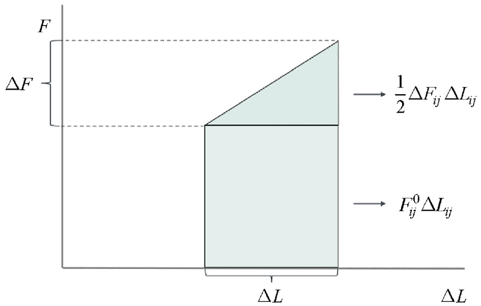
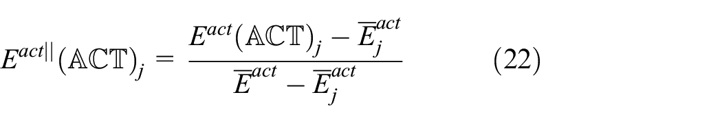
The actuation energy for control is a key metric for adaptive structures (Reksowardojo et al., 2022; Senatore et al., 2011). Assuming a linear elastic force-displacement relationship and small deformations, an estimate for the actuation energy (or control energy)
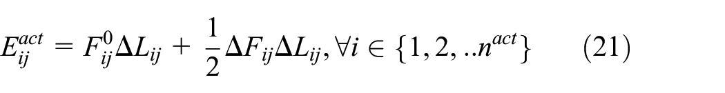
where
Control energy
The energy parameter
The operational energy lower bound
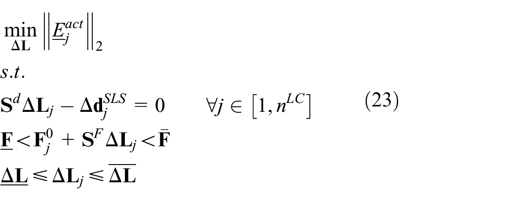
In equation (23) all elements are considered active, hence no placement integer variable is necessary. The only variable is the control command vector
Two metrics are adopted to assess the ability of a selected actuator set to satisfy the target control outputs: one is based on the compensability Gramian formulation in (Wagner et al., 2018), and the other on an efficacy measure formulated in (Senatore et al., 2019). The compensability quantifies the ability of a set of actuators to compensate for the effects of a generic disturbance on displacement or internal forces. Denote
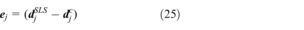
The compensability Gramian
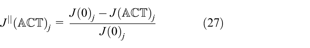
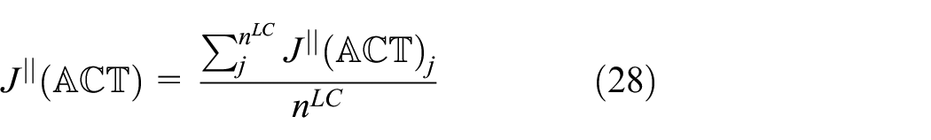
The efficacy of an actuator set
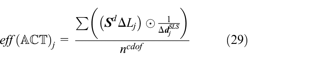
Alternatively, if the control objective is force compensation
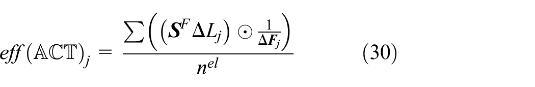
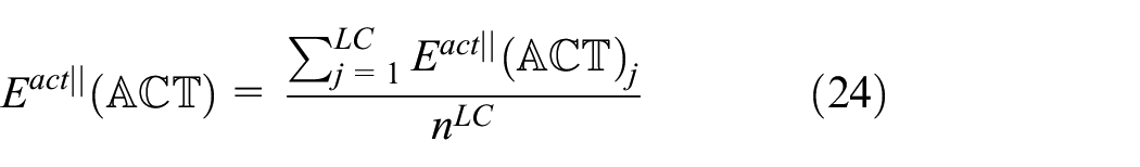
The symbol ⊙ denotes the Hadamard product (i.e. elementwise). The actuator set efficacy is then averaged for all load cases
The efficacy metric provides an average relative error for the controlled displacements, while the Compensability Gramian trace correlates with the average squared output error norm. This implies that using the efficacy metric will penalize even minor violations of the control targets compared to the Gramian-based metric, which instead gives a bias to absolute target errors, such as large displacements at the free end of a cantilever compared to those at the constrained end. In the context of the application of this metric for actuation placement, it is assumed that the uncontrolled state always violates serviceability conditions and that the controlled state should not overshoot the target displacements. This typically guarantees a smoother shape in the controlled state.
4.2. Sequential actuator placement formulation
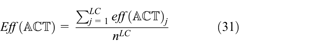
Most previous methods (e.g. Senatore et al., 2019; Wagner et al., 2018; Zeller et al., 2022) have adopted sequential approaches to formulate the actuator placement problem, which can be categorized under Stackelberg Game optimization (Ali et al., 2015; Marker and Bleicher, 2022; Wagner et al., 2018; Zeller et al., 2022). This consists of a sequential or bi-level process with two players that are referred to as the leader and follower. The process is represented diagrammatically in the flowchart in Figure 4. The same approach can also be thought of as a nested optimization. In the outer or “leader” the actuation binary vector is the optimization variable. A candidate actuator placement is therefore set in the lead process. Subsequently, in the nested or “follower” process, optimal control inputs are obtained for each candidate actuator layout. The process repeats iteratively to minimize a cost function. The cost functions considered in this work are the minimization of the actuator number and control energy. Depending on the formulation, these can be minimized directly (e.g. global search) or indirectly (local search). The optimal control inputs are determined by solving the constrained optimization problem stated in equation (16).
Sequential formulation flowchart.
4.2.1. Local search through integer relaxation (IR) and efficacy measure
An actuator placement method based on the efficacy measure outlined in Section 4.1 and constrained optimization is given in (Senatore et al., 2019). The number of actuators

This is the number of releases required to transform a statically indeterminate structure into a controlled mechanism (Senatore et al., 2019). However, a lower number of actuators can often be employed to satisfy displacement and stress limits, as also shown in (Senatore and Wang, 2024; Wang and Senatore, 2020). The actuator placement is performed by relaxing the integrality condition of the assignment variable adopting a sequential approach.
First, all elements are considered active, that is,
4.2.2. Local search through Greedy selection and compensability measure
Following (Wagner et al., 2018), a Greedy algorithm is implemented to solve the actuator placement problem. The performance metric adopted for the greedy search is the normalized compensability
Greedy algorithms, although simple to implement, typically produce sub-optimal solutions because the overall problem structure is not considered and there is no means of backtracking. When starting from a configuration where all elements are considered active, early-stage selection might not be effective because the performance metric
4.2.3. Global search
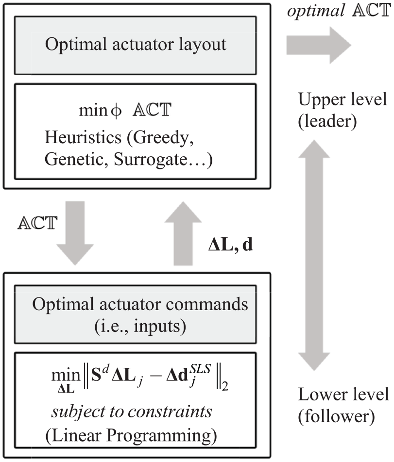
A critical limitation of approaches based on local search is that the actuator positions and the number of actuators are procedural variables that are determined sequentially. This causes a disconnection between the objective function minimization and constraint satisfaction. For example, solutions with a low number of actuators might be obtained with a significant deterioration of the constraint residuals. To overcome these limitations, global search approaches are implemented which provide a more robust strategy by exploring the search space more extensively. With these strategies, it is possible to consider the actuator positions as explicit design variables, which enables the incorporation of the number of actuators in the objective function as in equation (33). The objective also includes the compensability metric to obtain actuator placements that can satisfy the control target with small residuals.
Although the search is global, the optimization involves a nested process (the follower) to evaluate constraint satisfaction, the output of which must be considered in the objective function to steer the search towards feasible regions. Two methods are implemented for global search: a Genetic Algorithm (GA) and a Surrogate Algorithm (SA). In both cases, the objective function is given in equation (33) while the actuator commands are determined by solving the problem stated in equation (16). The GA employed in this work is the algorithm implemented in Matlab (Chipperfield and Fleming, 1995). Regarding SA, the objective function in equation (33) is evaluated for a set of candidate actuator layouts (i.e. sample points), which are used to make a surrogate through radial basis function (RBF) interpolation. The minimum of the surrogate function is employed as a new sample point to improve the interpolation. When the distance of the new minimum is within a certain tolerance to a previously obtained minimum, it means that the surrogate approximation is accurate, and a local minimum has been found. Subsequently, the search starts again using new sample points that are generated to explore a different region of the solution space. The surrogate model is employed to drive the search for the global optimum, allowing for efficient exploration of the solution space and identification of good regions where high-quality solutions are likely to be obtained (Mueller, 2014; Wang and Shoemaker, 2014).
4.3. All-In-One (AIO) actuator placement formulation
An All-In-One (AIO) formulation refers to solving a multi-variate and/or multi-objective optimization problem by obtaining all variables simultaneously. This typically requires an in-depth knowledge of the problem and a certain creativity in modeling all necessary equations simultaneously within a single problem statement. AIO formulations typically produce high-quality solutions because they can model interdependencies between variables such as the case of actuator positions and control commands.
4.3.1. Actuator number minimization
In this work, since the aim is to compare actuator placement methods, the structural parameters are pre-determined through a separate optimization process. The actuator placement problem is stated as
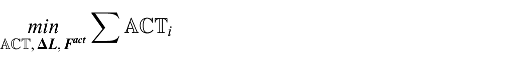


The optimization objective is the minimization of the number of actuators
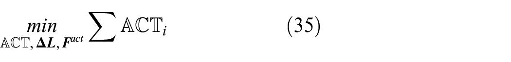
The design variable is the actuator assignment

where

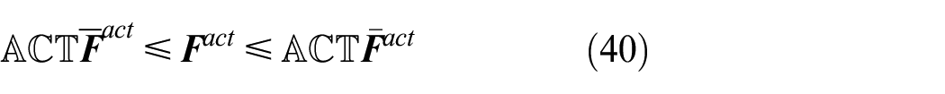
The actuator force variable
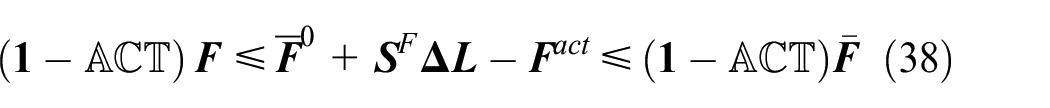
In this process

so that the element force
Actuator placement is avoided for elements that are subjected to a force in the uncontrolled state

Note that this constraint can be enforced when the structural parameters are known, that is, the structural sizing and topology are obtained through a separate process.
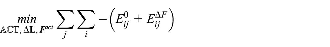
4.3.2. Energy minimization
The formulation given in equation (34) does not consider the control energy directly, which can be computed after a solution is obtained. To benchmark the quality of the solutions obtained through equation (34) concerning the control effort, an additional formulation is given in equation (42). The objective function is the minimization of the control energy that is stated in equation (21)


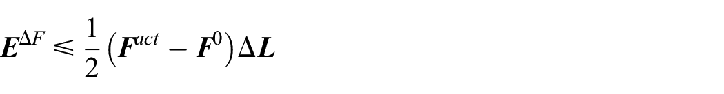


Referring to equation (21) for the control energy, only negative terms are accounted for to avoid considering energy gains. To eliminate discontinuities caused by absolute terms, two auxiliary variables are introduced

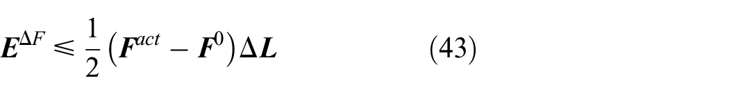
which will be satisfied with equality only when the solution of minimum energy is obtained. To avoid potential energy gains (positive work with the adopted sign convention), the variables


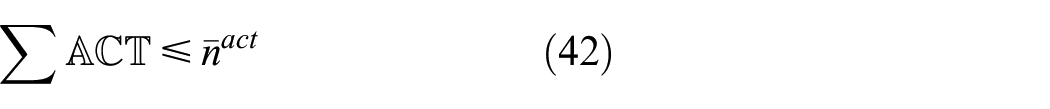
Limits on the number of actuators are formulated as
This way it is possible to evaluate solutions with the minimum number of actuators as well as actuator placements that require the least energy given a certain number of actuators that can be placed.
Since the actuator force is proportional to the length change via the force influence matrix
The eigenvalues of

(a) Non-convex bilinear function, (b) convex region of a non-convex bilinear function.
The computational complexity of MIP problems is typically exponential in the worst case due to the integrality of the variables. For the problems investigated in this work, the computational complexity is
4.3.3. AIO actuator placement problem solution
The AIO formulations stated in equations (34) and (42) have been successfully solved using the branch and bound algorithm implemented in Gurobi (Gurobi Optimization LLC, 2020). A branch and bound algorithm systematically explores the solution space in the form of a search tree by branching on discrete variables and solving linear or nonlinear programming problems to obtain feasible solutions (Bertsimas and Tsitsiklis, 1998). The solution of the continuous relaxation is referred to as lower Bound (LB), when it is integer feasible, it is referred to as an upper bound UB. The mixed-integer programming gap (MIP-gap) is defined as
When the gap is zero (i.e. UB = LB), it provides proof of the solution’s global optimality. For high-dimensional problems, the optimality of an integral solution might not be proved. MIP problems are known to be exponentially complex in the worst case, therefore, especially for problems with many integer variables, it is not always possible to prove global optimality. However, the MIP-gap can still be used to evaluate the solution quality.
The AIO formulation stated in equation (34) has also been solved using a mixed-integer Genetic Algorithm (GA) and Surrogate Algorithm (SA). Regarding the AIO-GA, different from sequential approaches, additional terms are added to the objective function to penalize unfeasible solutions that violate the constraints. The binary variable integrality is forced through heuristics that involve rounding feasible points to integers (Deb, 2000; Deep et al., 2009). Similarly, regarding the AIO-SA, the surrogate function is generated using sample points that at first satisfy constraints containing continuous variables only, and subsequently round the integer variables using a heuristic to preserve the constraint feasibility (Mueller, 2014; Wang and Shoemaker, 2014).
5. Case studies
The actuator placement methods presented in Section 4 are compared using numerical examples varying the number of structural elements, load cases and geometric dimensions. All case studies consider slender high-rise multi-story buildings modeled as pin-jointed trusses, which are shown in Figure 6.
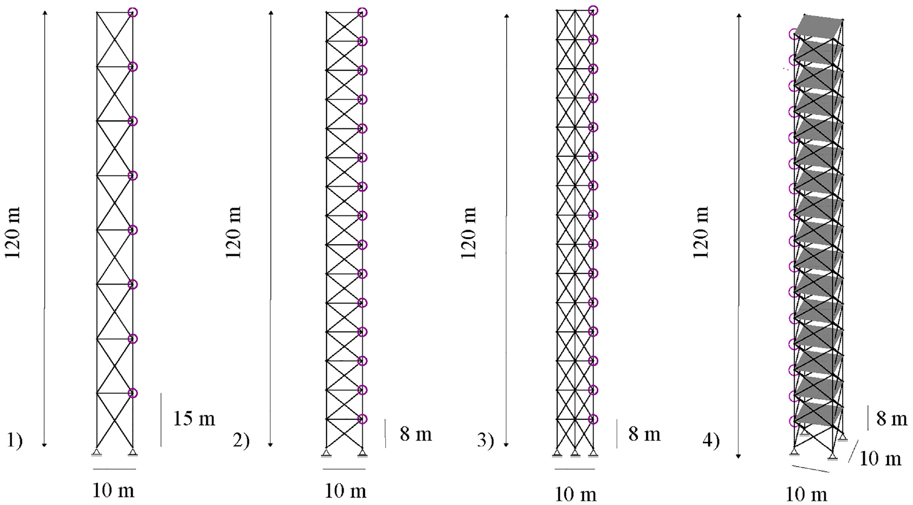
Dimensions and boundary conditions; controlled nodes are indicated with circles.
5.1. Geometry and loading
Three planar (2D) configurations with an increasing number of elements under two load cases and one spatial (3D) configuration under four load cases are considered. The structural and control parameters are given in Table 1. All elements are made of structural steel S355 and have cylindrical hollow sections with a wall thickness set to 10% of the external diameter. The minimum diameter is 100 mm.
Structural and control parameters.
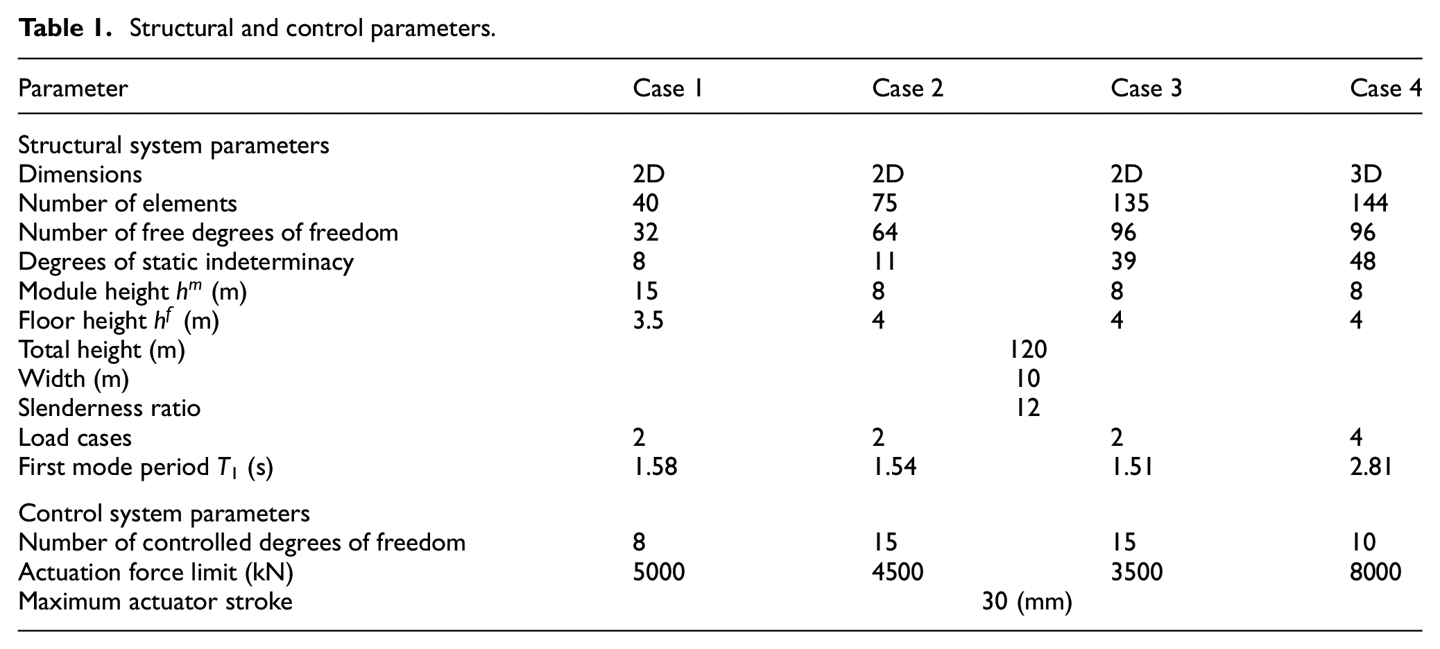
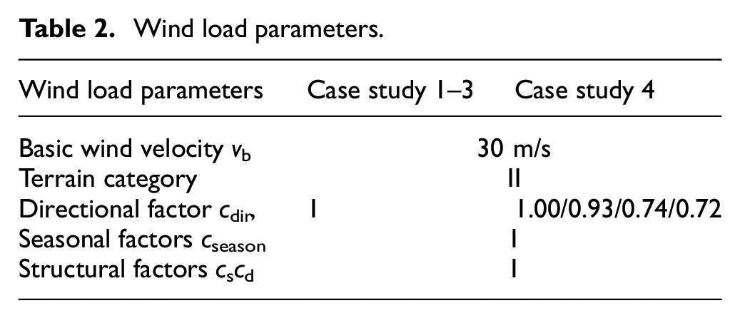
The self-weight (SW) is determined from the cross-section dimensions, and the dead load (DL) is set to 4,92 kN/m2 (500 kg/m2). The imposed live load (LL) is set to 2.94 kN/m2 (300 kg/m2). A wind load (WL) is also applied. The wind loads are computed according to EN 1991-1-4 considering a reference velocity v = 30 m/s, using the parameters given in Table 2. For the 2D cases, an out-of-plane dimension equal to the width of the structure is considered to determine the load influence areas. The floor height is set to 3.5 m for case study #1 and 4.0 m for case study #2, #3, and #4. Gravitational loads (SW, DL, LL) are applied according to the number of floors contained in each module, which are 4 for case study #1 and 2 for case study #2, #3, and #4. A prevailing wind direction is considered for case study #4 (3D) as indicated in Table 2.
Wind load parameters.
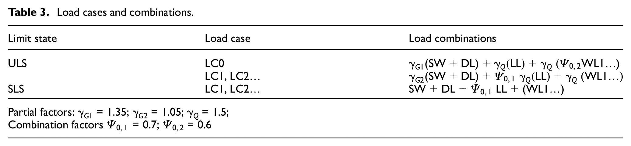
The design load combinations are given in Table 3.
Load cases and combinations.
For the 3D case (#4), a rigid diaphragm is employed to model each floor. The diaphragm assumption allows reducing the horizontal degrees of freedom to two translational and one rotational degree of freedom for each floor. To simplify the analysis further, the floor elements are omitted by applying internal translational and rotational constraints on the corresponding nodal degrees of freedom with respect to a floor master node. This model simplification results in a reduction of the free degrees of freedom from 198 to 96. The controlled degrees of freedom are indicated with circles in Figure 6. Thanks to the rigid diagram assumption, only one controlled degree of freedom per floor is sufficient for the 3D case study.
5.2. Structural design
The elements of the adaptive structures are sized to satisfy ultimate limit states (ULS), while serviceability limit states (SLS) do not have any influence on element sizing as they are satisfied through active control. The maximum stress under the ULS combination is limited to 80% of the yield stress. The reader is referred to (Senatore et al., 2019) for a detailed description of the sizing optimization process. To limit optimization complexity, global stability is not considered. The displacement limits are set to Hm/500 where Hm is the height of each module with respect to the ground. Figure 7 displays the deformed shapes under a single load case of the passive structures. For the passive case, the element cross-sections are sized to satisfy ULS and SLS requirements. Figure 8 illustrates the deformed shapes of the adaptive solutions in the uncontrolled state and gives mass savings compared to the passive solutions. Figure 9 illustrates the controlled displacement state.
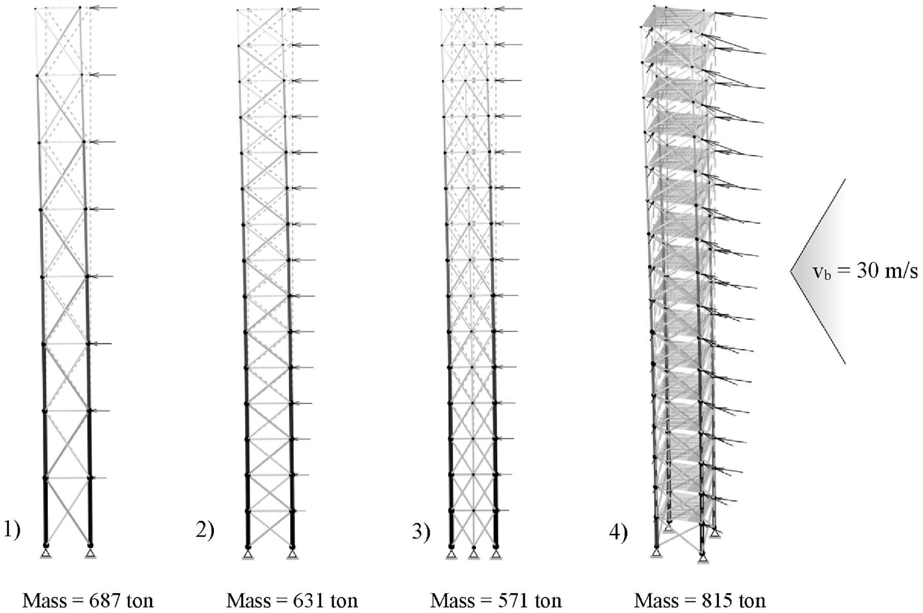
Passive systems: structural mass (primary structure only) and deformed shapes under a wind-load characteristic combination: (1) mass = 687 ton, (2) mass = 631 ton, (3) mass = 571 ton, (4) mass = 815 ton.
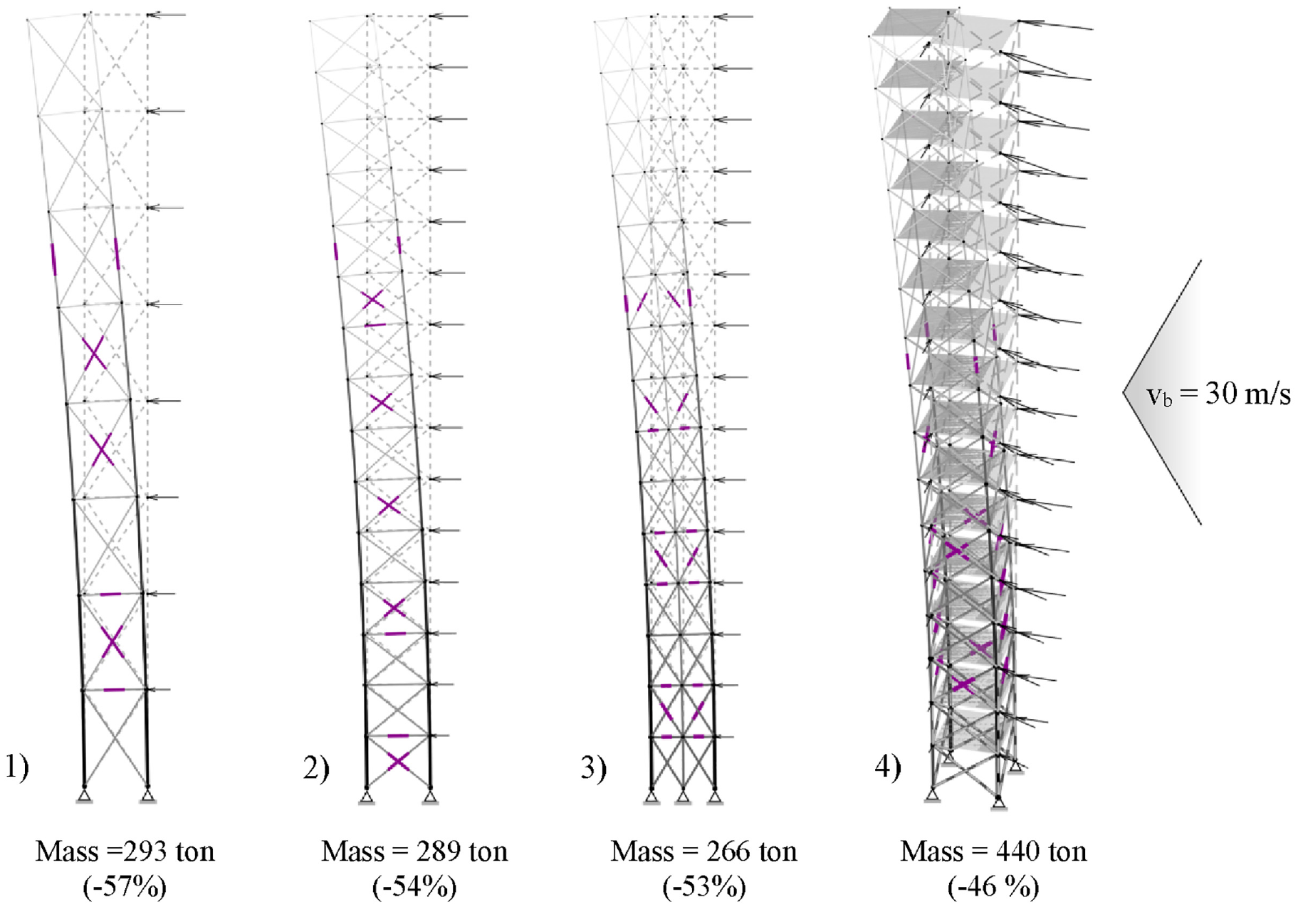
Adaptive systems: structural mass (primary structure only), mass savings, uncontrolled state under wind load characteristic combination; active elements are indicated with purple lines: (1) mass = 293 ton (−57%), (2) mass = 289 ton (−54%), (3) mass = 266 ton (−53%), (4) mass = 440 ton (−46%).
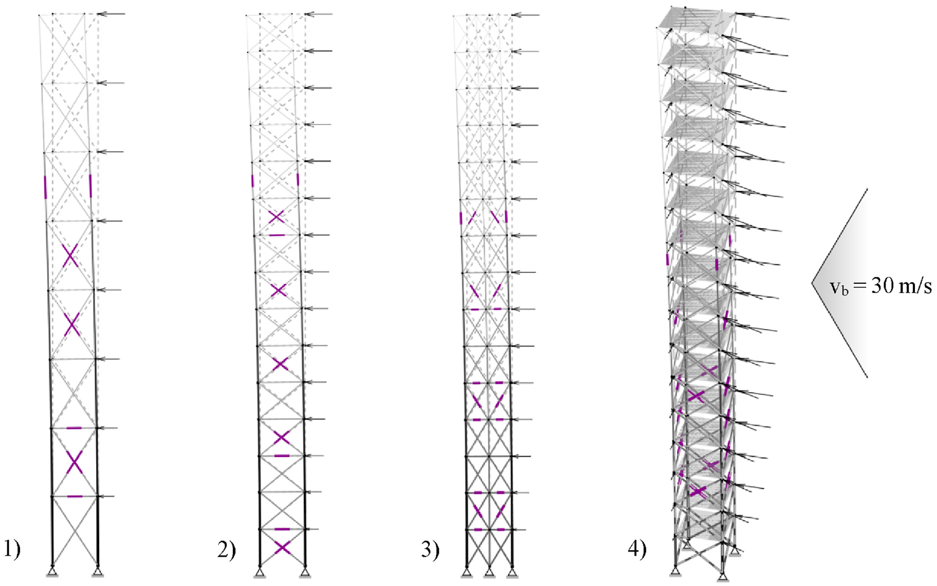
Adaptive systems: controlled state under wind load characteristic combination, actuator layouts obtained through the AIO formulation: (1) case study 1 (MIP-gap = 0.0%), (2) case study 2 (MIP-gap = 0.0%), (3) case study 3 (MIP-gap = 5.0%), (4) case study 4 (MIP-gap = 12.5%).
5.3. Actuator placement
The actuator placement is performed by implementing each method described in Section 4. The Integer Relaxation strategy
(a) Greedy-culling load-independent algorithm
(b) Greedy-culling load-dependent algorithm
(c) Greedy-additive load-dependent algorithm
(d) Genetic algorithm
(e) Surrogate algorithm
Greedy algorithms use the Compensability Gramian-based metric defined in equation (28) while Genetic and Surrogate algorithms adopt the objective function defined in equation (33) (see Section 4.2.3), where the weight coefficients are set to
The AIO formulation for the minimization of the actuator number in equation (34) is implemented using:
(a) Mixed-Integer Linear Programming
(b) Mixed-Integer Genetic algorithm
(c) Mixed-Integer Surrogate algorithm
The AIO formulation for the minimization of the control energy in equation (42) is implemented as a Mixed-Integer Quadratic Programming
Optimization solvers.
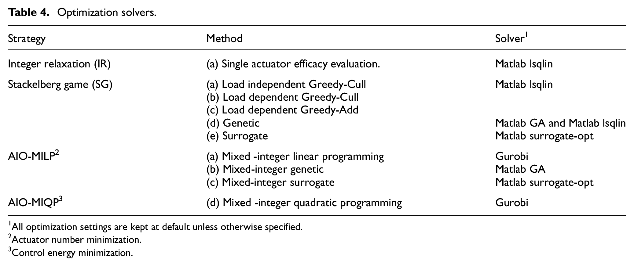
All optimization settings are kept at default unless otherwise specified.
Actuator number minimization.
Control energy minimization.
Referring to the problems stated in equations (16), (34), and (42), a tighter constraint on control feasibility concerning element stress and actuation forces is applied by reducing the tolerance on inequality conditions to 1e-5. Instead, since displacement control is not a safety-critical condition, the related tolerance is relaxed by allowing the controlled node position to be in the range expressed in equation (48)
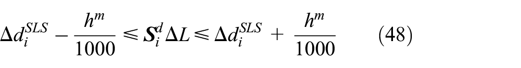
where
For the methods IR, SG(a), SG(b), SG(c), the number of actuators
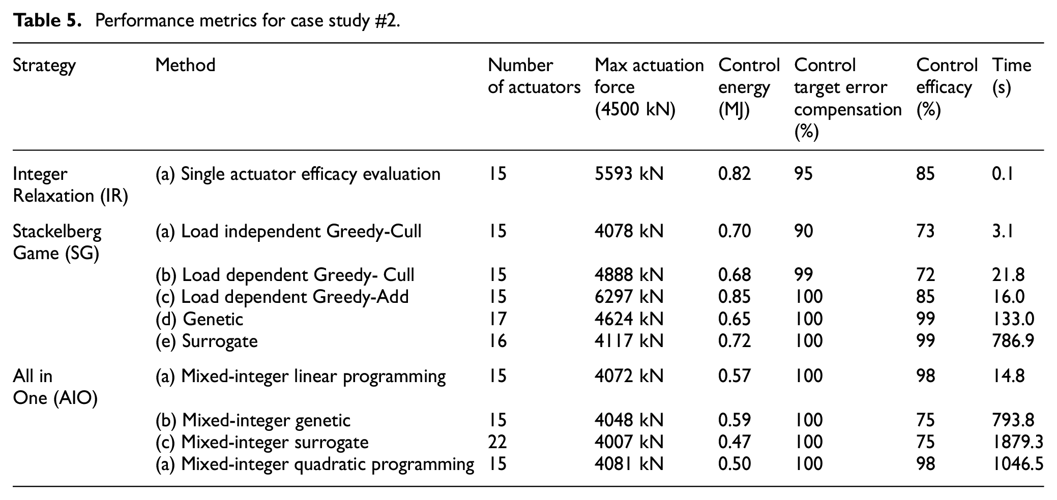
Table 5 gives optimization metrics for all placement methods for case study #2 which is taken as an illustrative case. Due to the tight tolerance limits on internal stresses and actuator length changes, the solutions provide feasible control inputs that guarantee structural integrity at the expense of the displacement target attainment. The performance of each method is evaluated considering (a) the number of actuators, (b) the maximum actuator force (c) the control energy (d) the absolute displacement error compensation, (e) the control efficacy, and (f) the computational time. Sequential and heuristic approaches, often produce feasible solutions only if constraints on the maximum actuation forces are relaxed to some extent.
Performance metrics for case study #2.
For methods implementing Genetic algorithms (
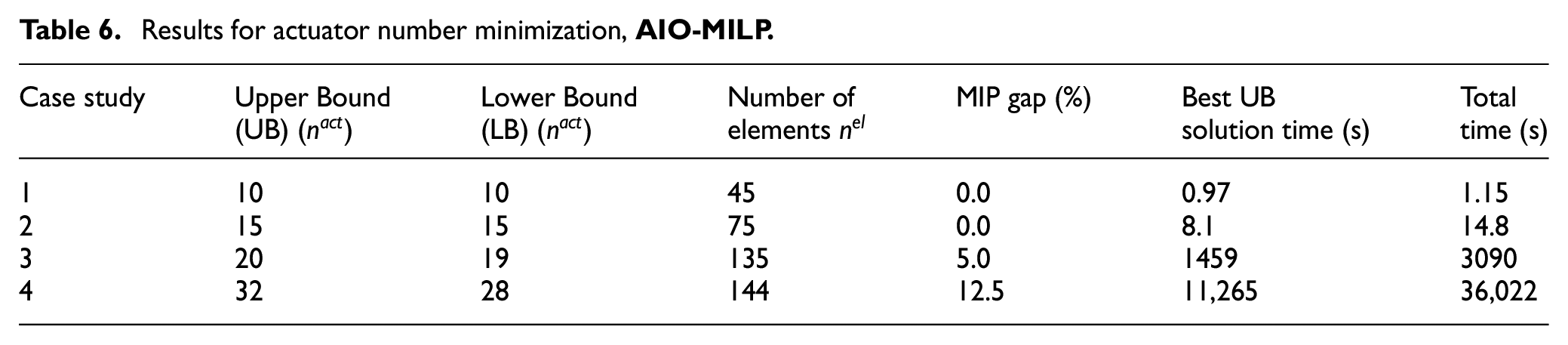
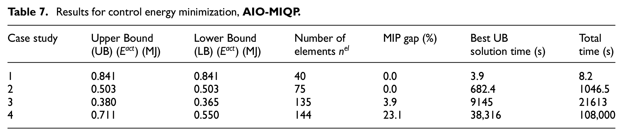
Table 6 gives upper and lower bounds for the MILP solutions for each case study. Table 7 gives upper and lower bounds for the MIQP solutions for each case study. Figure 10 shows the control energy savings obtained through
Results for actuator number minimization,
Results for control energy minimization,
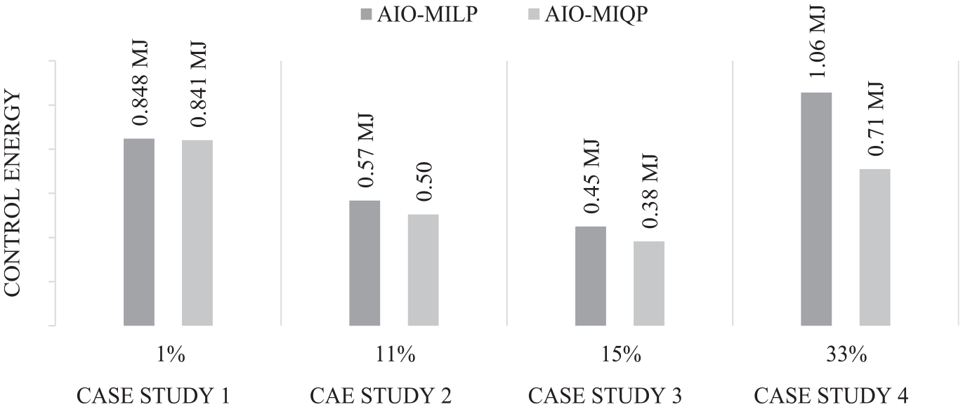
Control energy saving obtained through AIO-MIQP (control energy minimization) with respect to AIO-MILP (actuator number minimization).
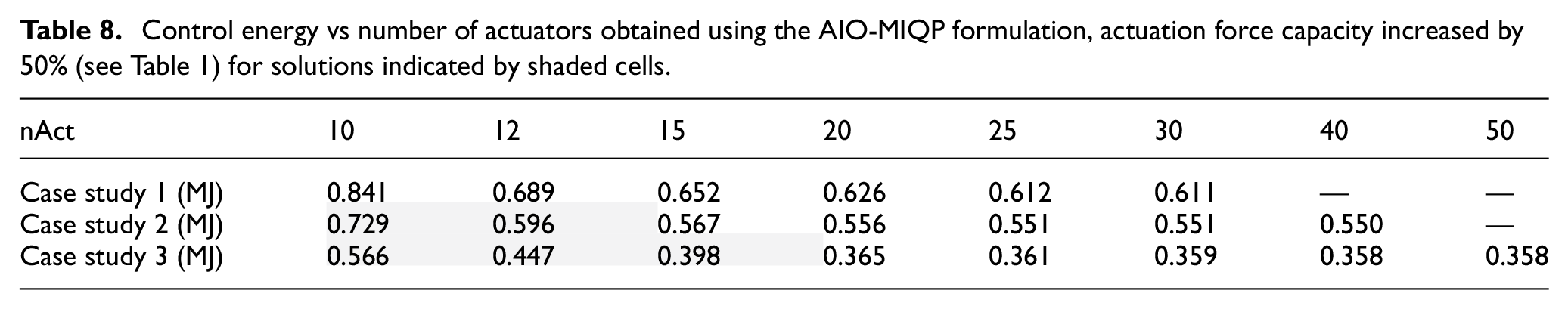
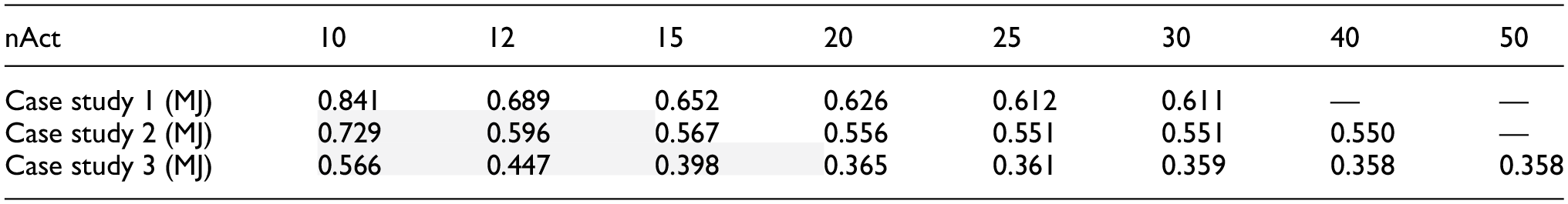
For case studies #1 to #3, a Pareto analysis has been performed progressively increasing the number of actuators in formulation (42) until actuation force limitations prevent further actuator assignments. Figure 11 shows the Pareto fronts control energy vs number of actuators. For clarity, the value of the control energy optimization (AIO-MIQP) are also given in Table 8. Generally, the required control energy decreases asymptotically as the number of actuators increases. This is expected since the minimum control energy is obtained when all elements are active (see Section 4.1). The discrepancy in the control energy magnitude between the three cases can be attributed to the varying stiffness levels, as the degree of redundancy increases from case #1 to case #3. This study gives a rigorous confirmation, since the solutions are global optima, of the trend that was already observed in (Senatore and Reksowardojo, 2020). Note that for case studies #2 and #3, when the maximum actuator number is below 15 and 20, respectively, it is necessary to increase the maximum actuator force to obtain feasible solutions, hence the corresponding Pareto curves are indicated with a dashed pattern.
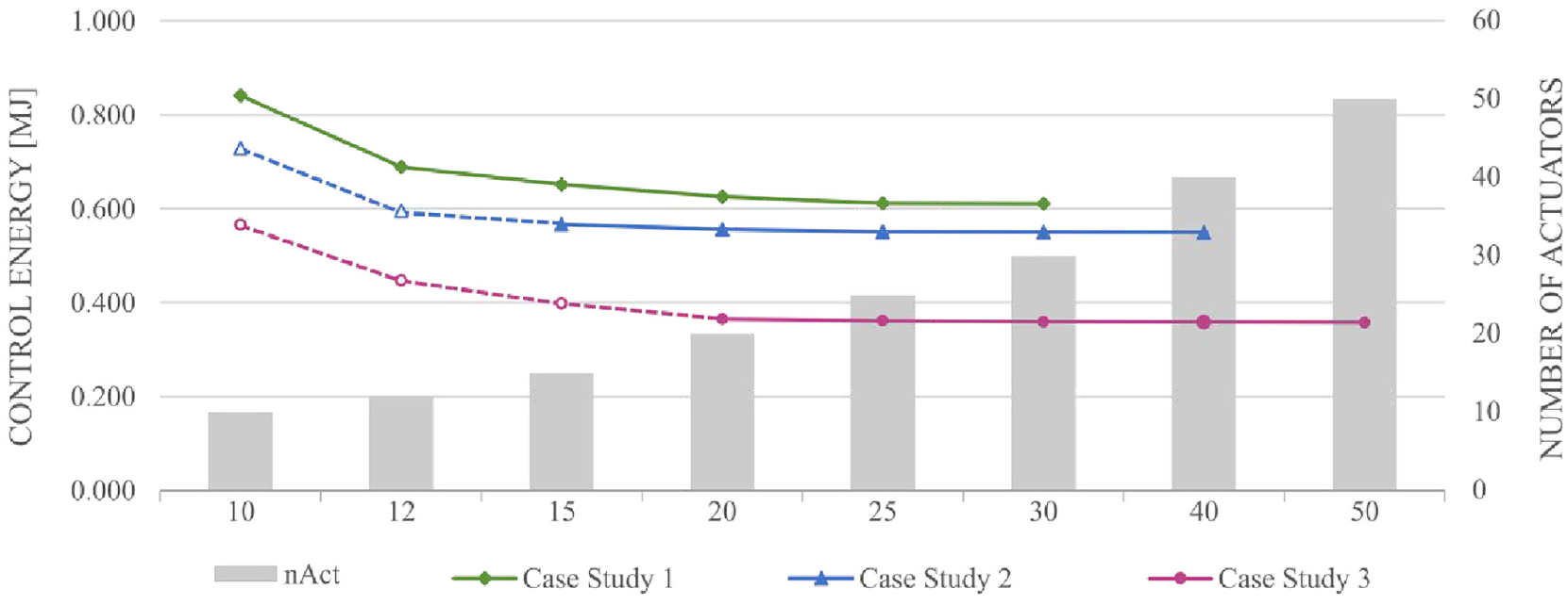
Pareto fronts control energy vs number of actuators obtained using the AIO-MIQP formulation.
Control energy vs number of actuators obtained using the AIO-MIQP formulation, actuation force capacity increased by 50% (see Table 1) for solutions indicated by shaded cells.
5.4. Benchmark
For a rigorous benchmark, for each case study k, all metrics
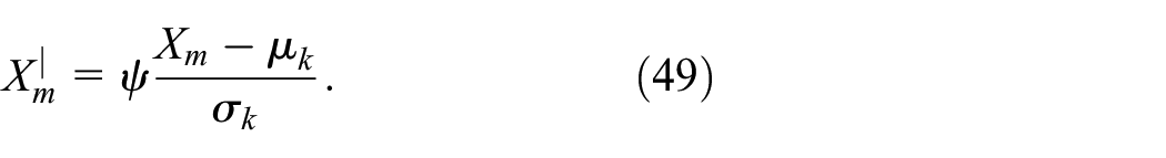
where
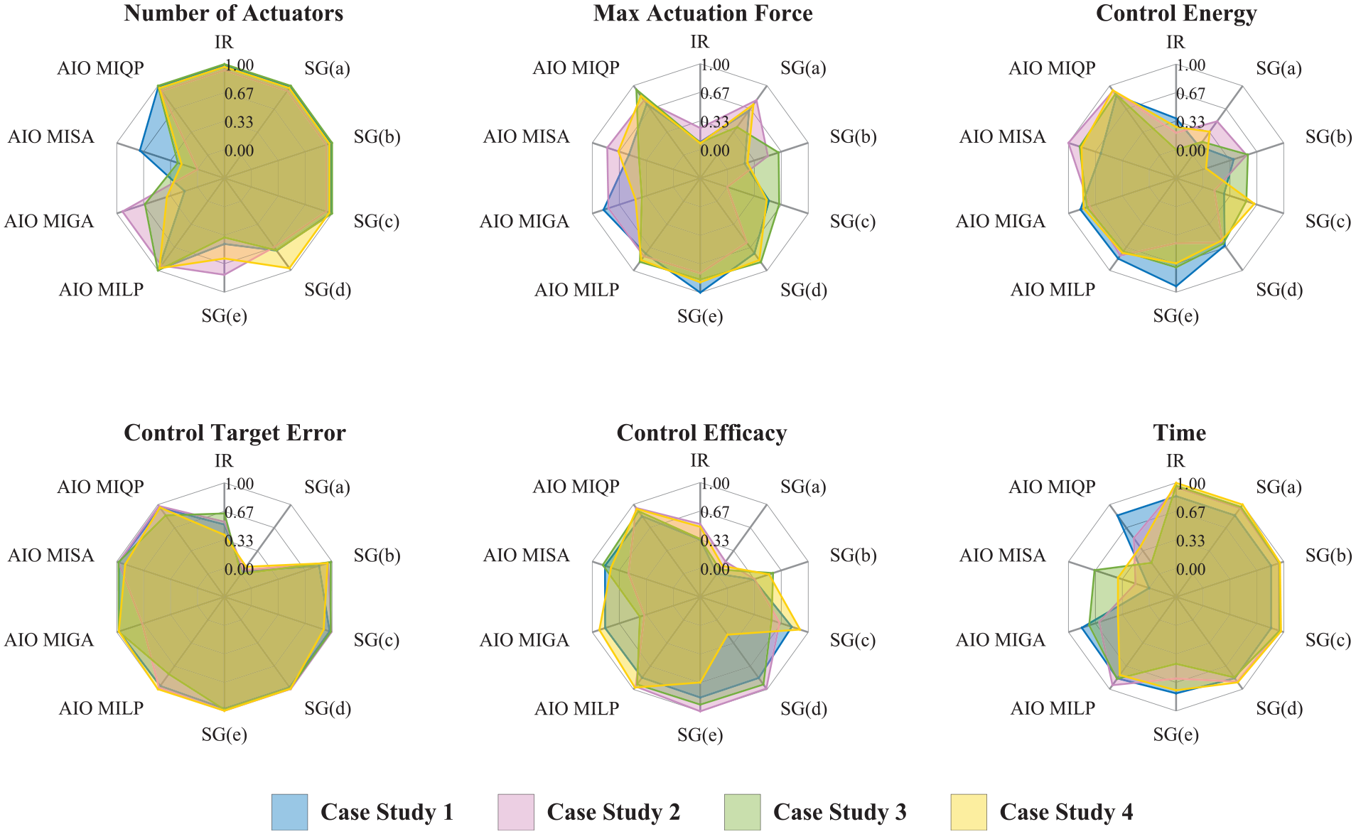
Performance metrics, standardized and normalized across all case studies.
To offer a more concise overview of the performance of each placement method, results are averaged across all case studies and metrics. The standard deviation of the optimization performance for each method across the case studies gives an indication of the “reliability” of each method, that is, with what variability each method performs better or worse with respect to others. The computational time parameter is considered separately. The radar charts of the three global parameters are shown in Figure 13. The method
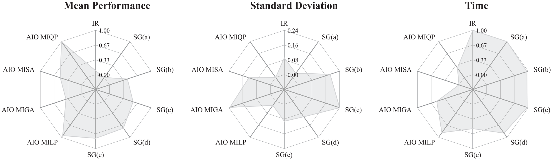
Mean performance, standard deviation, mean normalized process time.
Additional insights are given in Figure 14 showing the number of actuators for each method and case study that is required to satisfy control constraints within the assigned tolerance. For clarity, control constrain tolerances are satisfied for methods in which
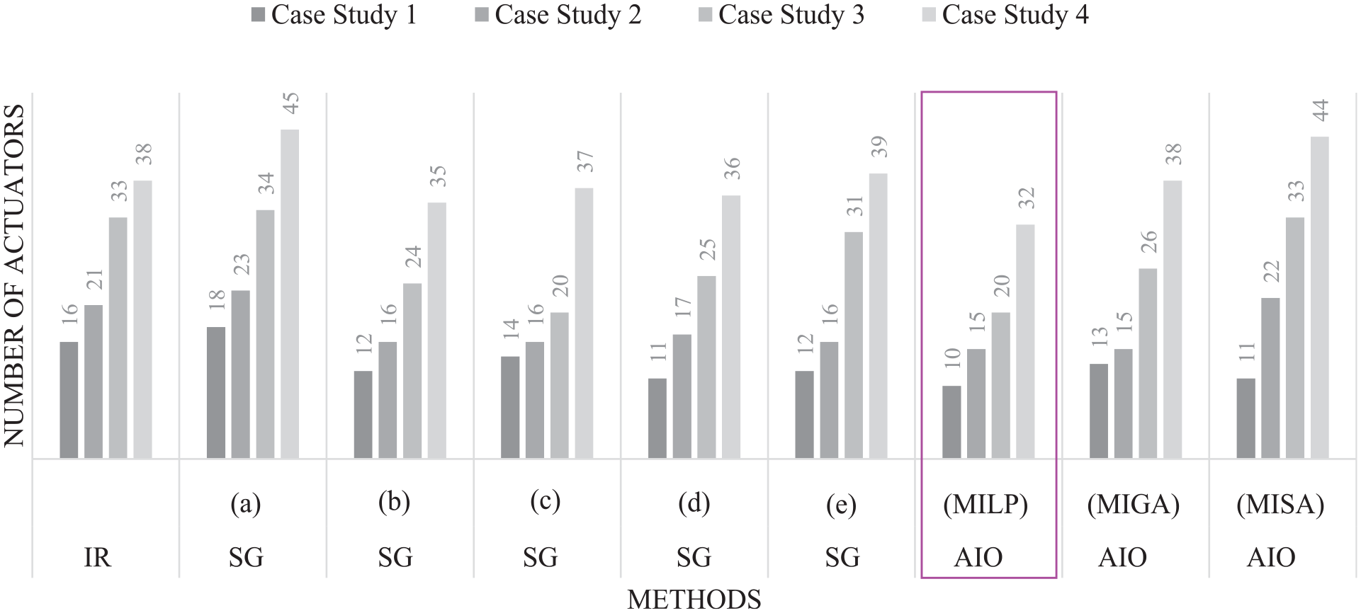
Number of actuators for each method and case study to satisfy displacement constraints within the assigned tolerance.
6. Discussion
Actuator layouts produced by methods that consider specific load cases have a significantly higher performance compared to methods that are independent of the disturbance
Stackelberg Game strategies that implement greedy selections as lead player tend to converge rapidly. However, the solution quality is significantly lower compared to the global search approaches such as Genetic Algorithm
AIO solutions implemented through metaheuristic approaches (
The computational time required by
The solutions obtained through the formulation stated in (34) (
7. Conclusions
Depending on the control objective and requirements, different metrics and constraints can be considered for actuator placement in adaptive structures. Actuator layouts produced by considering only displacement or force compensability separately are often not practical due to power and actuation force constraints. Since the design of a civil structure is typically carried out under the assumption of well-defined load cases, it is convenient that the actuator placement follows the same approach. This work has shown that actuator placement considering specific load cases, produces better-quality solutions in terms of control efficacy and feasibility.
Genetic and Surrogate algorithms perform best in sequential approaches using the actuator positions as design variables of the lead player and control inputs obtained in the follower player using constrained least square optimization. The AIO-MILP and AIO-MIQP formulations produce actuator layouts with the lowest number of actuators and the smallest control energy, respectively, required to satisfy structural integrity, serviceability, and control feasibility. For problems with many variables, due to computational limits, it might not be possible to verify global optimality. However, results have shown that, generally, the AIO upper-bound solutions (MIP gap < 30%) perform significantly better compared to the solutions produced by any other strategy tested in this work.
It has been proved numerically that the control energy decreases asymptotically as the number of actuators increases, which confirms the results obtained in previous work. However, the study carried out in this work offers rigorous numerical proof since the solutions considered in the Pareto analysis are global optima.
The formulations presented in this work can be extended to frame and shell structures. The main limitation is the number of variables that would be required for structures comprising beams and shells, which is significantly higher than for trusses, therefore model reduction techniques would be required. Future work will develop extension to include explicit consideration of dynamic actions (e.g. earthquakes) and control objectives will be formulated to include closed-loop performance parameters for vibration damping.
Footnotes
Appendix
Declaration of conflicting interests
The authors declared no potential conflicts of interest with respect to the research, authorship, and/or publication of this article.
Funding
The authors disclosed receipt of the following financial support for the research, authorship, and/or publication of this article: This work has been funded by the German Research Foundation (DFG-Deutsche Forschungsgemeinschaft) as part of the Collaborative Research Center 1244 (Project-ID 279064222–SFB 1244) Adaptive Skins and Structures for the Built Environment of Tomorrow.