Sage Journals: Discover world-class research

Abstract

The acoustic emission (AE) technique is commonly utilized for identifying source mechanisms and material damage. In applications requiring numerous sensors and limited detection areas, achieving significant cost savings, weight reduction, and miniaturization of AE sensors is crucial. This prevents excessive weight burdens on structures while minimizing interference with structural integrity. Thin Piezoelectric Wafer Active Sensors (PWAS), compared to conventional commercially available sensors, offer a miniature, lightweight, and affordable alternative. The low signal-to-noise ratio (SNR) of PWAS sensors and their limited effectiveness in monitoring thick structures result in the decreased reliability of a single classical PWAS sensor for damage detection. This research aims to enhance the functionality of PWAS in AE applications by employing multiple thin PWAS and performing a data-level fusion of their outputs. To achieve this, as a first step, the selection of the optimal PWAS is performed and a configuration is designed for multiple sensors. Pencil break lead (PBL) tests were performed to investigate the compatibility between selected PWAS and traditional WSα and R15α sensors. The responses of all sensors from different AE sources were compared in both the time and frequency domains. After that, convolutional neural networks (CNNs) combined with principal component analysis (PCA) are proposed for signal processing and data fusion. The signals generated by the PBL tests were used for network training and evaluation. This approach, developed by the authors, fuses the signals from multiple PWAS and reconstructs the signals obtained from conventional bulky AE sensors for damage detection. Three CNNs with different architectures were built and tested to optimize the network. It is found that the proposed methodology can effectively reconstruct and identify the PBL signals with high precision. The results demonstrate the feasibility of using a deep-learning-based method for AE monitoring using PWAS for real engineering structures.

Keywords

PWAS acoustic emission sensing data fusion principal component analysis conventional neural network

1. Introduction

An in-situ monitoring system should be able to undertake a proper assessment of residual life and evaluate the degradation of structural components (Nair and Cai, 2010) as well as to change the maintenance paradigm from scheduled maintenance to condition-based maintenance (CBM) (Nokhbatolfoghahai et al., 2022). The rapid development of infrastructure and technological advances has led to a growing interest in Structural health monitoring (SHM). Acoustic emission (AE) is one of the most promising non-destructive testing (NDT) techniques in the field of SHM (Barile et al., 2020; Calabrese and Proverbio, 2020; Carrasco et al., 2021; He et al., 2021; Nair and Cai, 2010; Saeedifar and Zarouchas, 2020; Verstrynge et al., 2021). AE technology relies on the radiation of acoustic (elastic) waves in a medium. The elastic waves are produced by the energy released due to suddenly internal deformation in a material, such as plastic deformation, crack formation/expansion, fiber breakage, delamination in composites, impact etc. An AE system is normally made up of sensors, preamplifiers, and data acquisition devices. The AE sensors are mounted on the surface of the material, as shown in Figure 1 (Cheng et al., 2022). Surface motions f(t) produced by the elastic waves are transformed to electronic signals a(t) by transfer functions, which can be mathematically represented as

a (t) = f (t) * w (t) * w_{f} (t) * w_{a} (t)

(1)

Where w(t), w_f(t), and w_a(t) are the time transfer functions of AE sensors, filters, and preamplifiers. These collected signals can yield useful information for SHM at different levels, including signal identification, damage localization, and life prediction. The frequency responses of the filters (w_f(t)) and amplifiers (w_a(t)) are commonly characterized by flat or constant responses (Grosse and Ohtsu, 2008). This implies that the recorded AE signal a(t) is highly sensitive to w(t) corresponding to different AE sensors. Thus, the sensitivity of the AE sensors is critical for AE monitoring.

Figure 1.

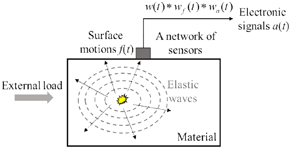
Acoustic emission (AE) principle (Cheng et al., 2022) where w(t) is the transfer function of the AE sensor, w_f(t) is the transfer function of the filter, and w_a(t) is the transfer function of the amplifier.

AE-emitted signals are often recorded using high-sensitive piezoelectric sensors with the main frequency response within the 20 kHz to 1 MHz range. In conventional AE sensors, a PZT (Lead Zirconate Titanate) element is often enclosed in a stainless-steel housing to enhance sensitivity response (see Figure 2) (Nakamura, 2016). They also have a detection face with wear plate to improve the electrical isolation from the tested object. These conventional sensors have been successfully used in a variety of structures (Chen et al., 2020; Cheng et al., 2021; Joseph et al., 2021; Liu et al., 2018; Wotzka and Cichon, 2020; Yu et al., 2013). However, detecting AE signals with conventional sensors has inherent disadvantages, such as their bulky size and high cost. It is infeasible to apply large quantities of conventional AE sensors to the structure due to the high costs of the monitoring. Meanwhile, the non-negligible mass/volume of the sensors hinders their practical applications, especially for in-situ SHM (Theses et al., 2017). Bulky AE sensors can be intrusive and potentially disturb the normal operation and functionality of the monitored structure, particularly in aerospace applications (Giurgiutiu, 2020). Furthermore, a real-world example illustrating the potential application of AE in restricted access areas is shown in Figure 3. This is an innovative C1 wedge connection used in offshore wind turbine (OWT) structures (Creusen et al., 2022). To ensure the reliability of this connection and prevent catastrophic failure, it is of paramount importance to have an effective method for early fatigue crack detection in this connection. However, the limited available space, with a height of less than 1 cm, makes it impossible to install conventional bulky AE sensors in the desired areas.

Figure 2.

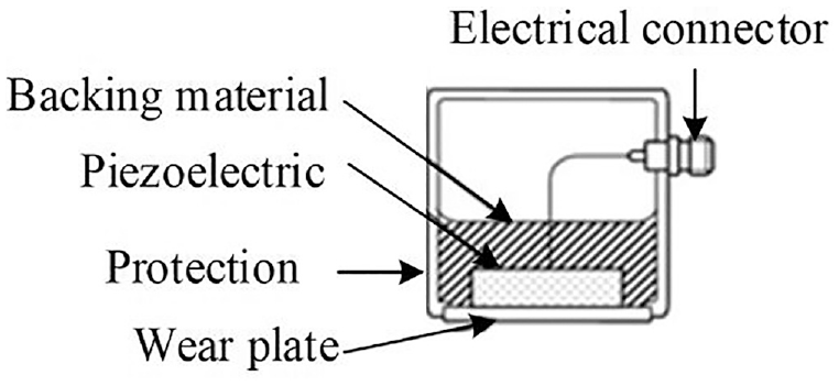
Typical structure of a conventional PZT bulky AE sensor (Nakamura, 2016).

Figure 3.

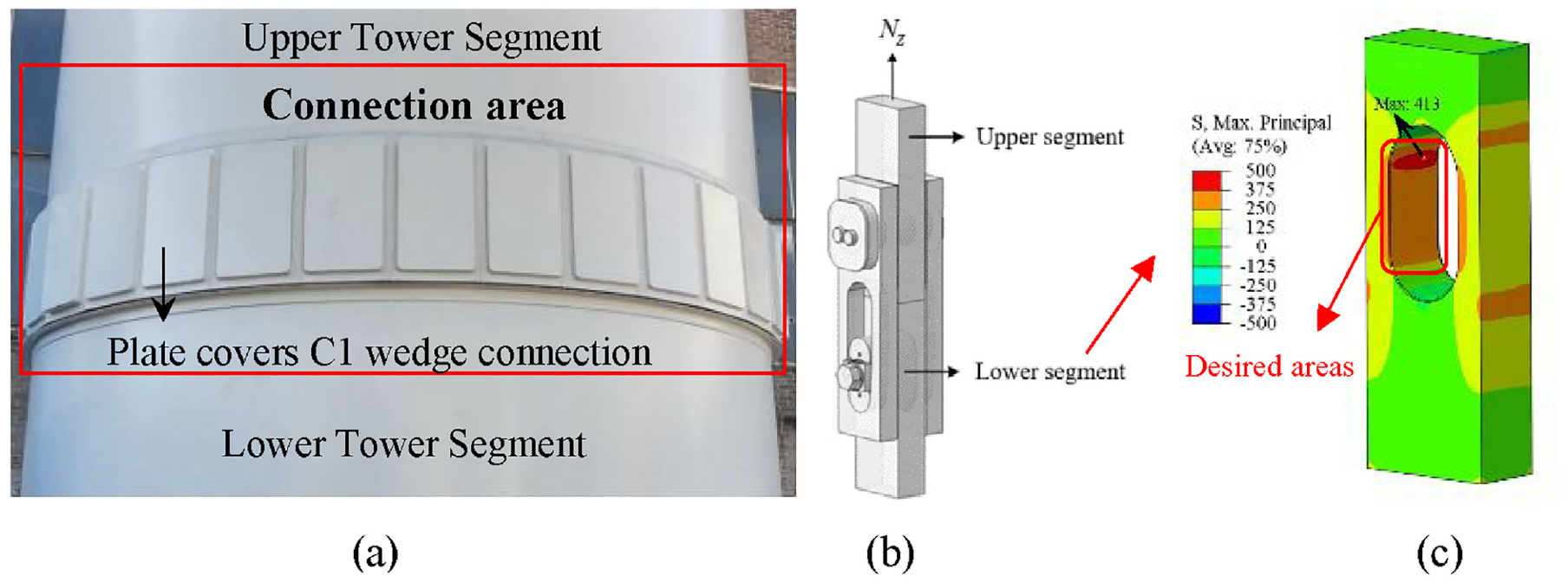
The C1 wedge connection: (a) covered by corrosion protection plates in the OWT structure (Creusen et al., 2022), (b) lay-out of the connection, (c) principal stress distribution of the lower segment (the critical component).

PWAS (Piezoelectric wafer active sensors) are miniature, low-cost, and lightweight, with several millimeters in height and a broadband response frequency. PWAS work well for both exciting and detecting ultrasonic guided waves in SHM (Giurgiutiu, 2007; Giurgiutiu and Zagrai, 2000). The installation process of PWAS can be complex and time-consuming, requiring expert knowledge and skills for proper placement and wiring. Over the past decade, numerous studies have demonstrated the feasibility of monitoring acoustic emissions with PWAS (Bhuiyan et al., 2018; Jiang et al., 2018; Yu et al., 2012; Zhang et al., 2020). Compared to commercial sensors, PWAS can deliver equivalent detection findings regarding fatigue cracks in thin plate-like materials. However, PWAS sensors are less effective for monitoring the thick steel plate where they have only captured 5% of the AE events of recorded by R15I sensors (Yu et al., 2011). Additionally, the analysis and comparison between conventional and PWAS are typically performed without any prior selection study for PWAS in passive sensing applications (Trujillo et al., 2014; Yu et al., 2012). Due to a lower signal-to-noise ratio (SNR), noise significantly impacts the efficiency of PWAS, hindering its performance. Furthermore, relying solely on measurements recorded by a single type of small PZT sensor may result in incomplete information regarding the underlying damage mechanism (Gall et al., 2018; Godin et al., 2018; Hamam et al., 2019). Using a single type of PWAS for AE monitoring has limited effectiveness, but it remains a viable alternative for monitoring critical areas with restricted access. To enhance the accuracy of passive AE monitoring using PWAS, it is essential to implement an optimized configuration of multiple PWAS along with advanced signal processing methods.

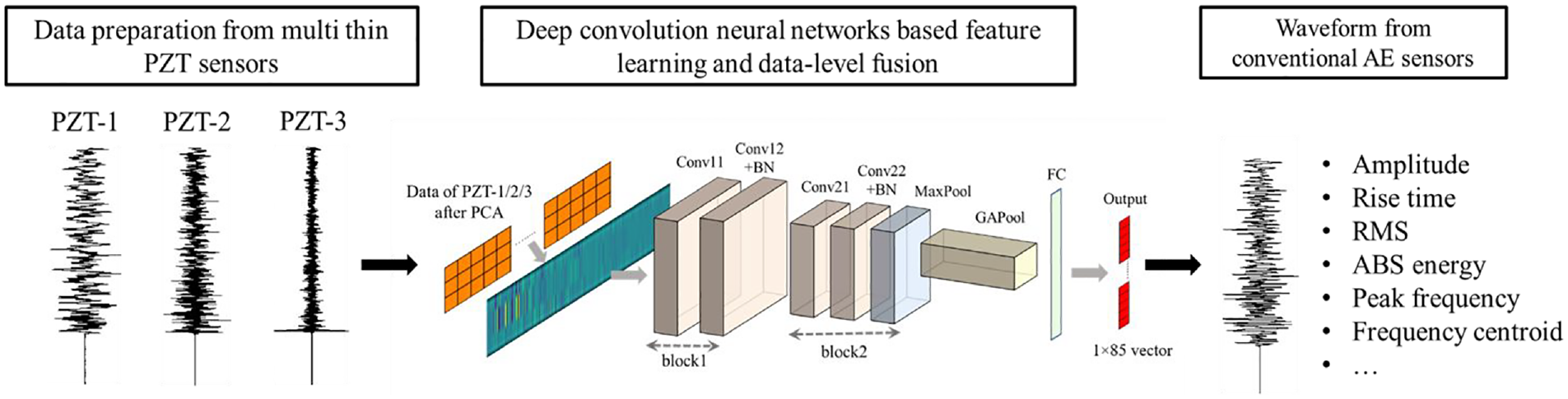
Data fusion can extract information from the combination of different datasets instead of analyzing each dataset separately (Wu and Jahanshahi, 2018). Previous works demonstrate the efficiency of combining data from multiple sensors to increase the accuracy and dependability of collected information. It is recommended to implement feature-based data fusion if the original data contain clearly distinguishable and adequate detectable features. In the case of an AE application with PWAS, data-level fusion is preferable since the original raw data from one type of PWAS cannot represent the essential characteristics of the damage mechanisms. However, the majority of research about multi-sensor data fusion has been performed at the feature level (Broer et al., 2021; Dehghan Niri et al., 2013; Guel et al., 2020; Liu et al., 2020; Saboonchi et al., 2016). Considering the higher SNR ratio of conventional bulky AE sensors, this study proposes a data-level fusion approach to reconstruct the signals from traditional AE sensors via the signals from PWAS (see Figure 4). Compared to other available approaches, deep-learning-based approaches have been applied in a range of academic domains for image processing. Although 1D-CNNs can apply to time-series data, Wu et al. (2018) have reported that 2D-CNNs perform better than the 1D-CNNs method and achieve higher accuracy and robustness. To enhance the efficiency of data-level fusion using CNN, PCA is used to minimize the dimensionality of the obtained waveforms without losing critical signal information. Dimensionality-reduced signals extracted from selected PWAS are saved as image files, which are then used as input data for the 2D-CNN. The output consists of waveforms derived from PCA-processed signals of conventional bulky sensors.

Figure 4.

A flowchart illustrating the proposed data-level fusion approach.

This work explores the implementation of PWAS of different sizes for AE monitoring. The selection of PWAS is performed according to the proposed criteria, aiming to enhance the completeness of the collected data. A detailed experimental analysis using Pencil break lead (PBL) tests on a compact-tension (CT) specimen is conducted to test the interchangeability between different types of sensors for AE monitoring. After that, we utilize a combination of multivariate analysis based on principal component analysis (PCA) and convolutional neural network (CNN) to fuse the signals from different PWAS. Finally, the performance of the established CNN is evaluated with extracted features.

This paper is organized as follows: In Section 2, a brief methodology overview is presented. Sections 3 and 4 describe the experimental setup and discussion. Section 5 details the proposed methodology for data fusion of multiple PWAS and evaluates its performance. The conclusions are drawn in Section 6.

2. Overview of theoretical background

To explain the concept of the proposed methodology in more detail, Section 2 is divided into three parts. The most employed acoustic emission signal features are briefly explained in Section 2.1. An introduction to the CNN architecture is given in Section 2.2. Then Principal Component Analysis (PCA), which is utilized for dimensionality reduction of the input of the established CNN, is presented in Section 2.3.

2.1. Acoustic emission signal features

SHM with the AE technique is properly explained by AE signal parameters. Figure 5 shows the most widely used AE features in the time domain. Frequency-domain features also play a significant role in interpreting AE signals. Representative parameters are the peak frequency (PF) and the frequency centroid (CF). Besides, AE signals can be described more precisely by the partial power (PP) features which measure the ratio of power in a user-specified frequency range (f₁ – f₂) to the complete power of a signal:

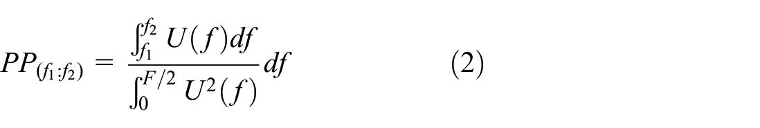
P P_{(f_{1} : f_{2})} = \frac{\int_{f_{1}}^{f_{2}} U (f) df}{\int_{0}^{F / 2} U^{2} (f)} df

(2)

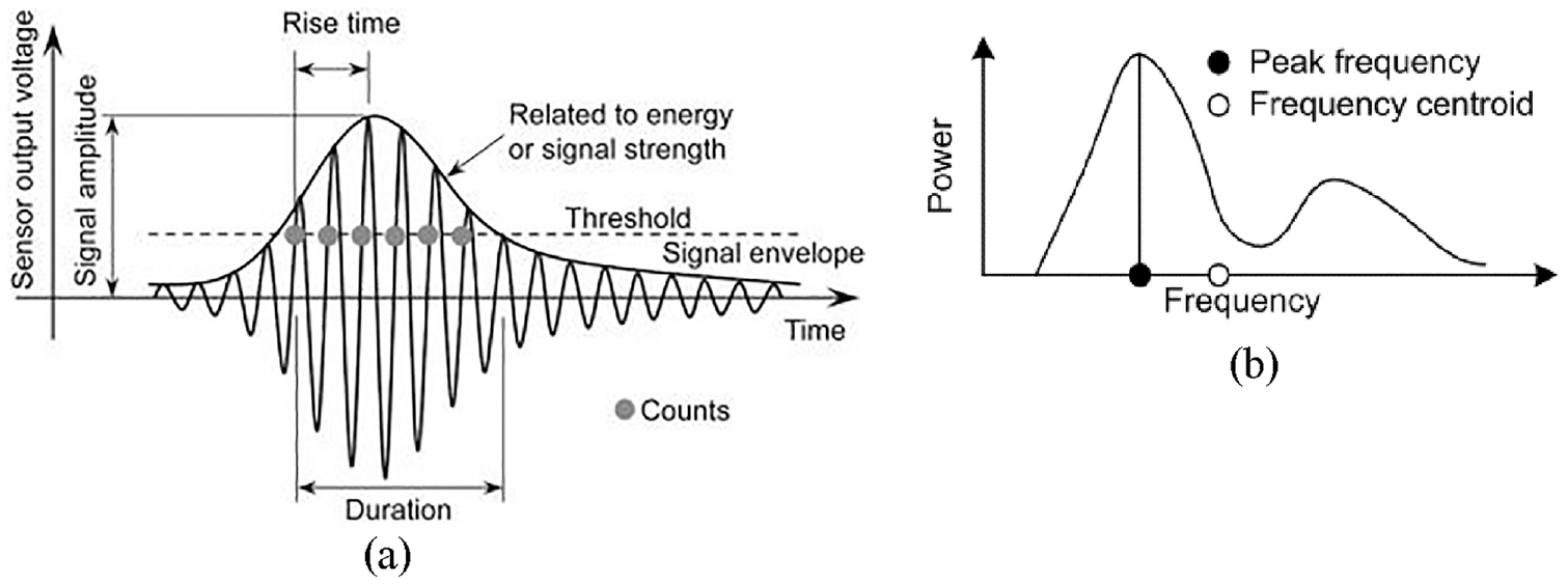
Where a power spectral density formula $U (f)$ is obtained using FFT from each signal, and F is the sampling frequency of the signals. More detailed information about AE signal features can be found in reference (Grosse and Ohtsu, 2008).

Figure 5.

Conventional AE features in (a) time domain (ElBatanouny et al., 2014), (b) frequency domain (Grosse and Ohtsu, 2008).

2.2. Convolution neural network

The convolutional neural network (CNN) is a powerful tool for feature extraction and image analyses. In contrast to traditional Artificial neural networks (ANNs), CNN takes advantage of local connections, shared weights, and sub-sampling. These operations enable the CNN model to extract representations of the image automatically at a low computational cost. CNN is designed to process data from different arrays, such as 1D data like signals and sequences, 2D data for pictures or spectrograms, and 3D image data like computerized tomography scans.

A typical CNN model can be found in Figure 6. It consists of three main kinds of layers, that is, a convolutional (Conv) layer, a pooling layer and a fully connected (FC) layer (Xin et al., 2020). A convolutional layer contains multiple filter kernels to extract local features over the whole image by the sliding process. These obtained features are then triggered by a non-linear function such as Sigmoid, Tanh, and rectified linear unit (ReLU). ReLU is the most frequently used activation function due to its simple implementation and less susceptibility to vanishing gradients (Alom et al., 2019). Local response normalization (LRN) layers execute a mathematical operation on the n × n area to constrain the unbounded nature of ReLU. To address the issues of internal covariate shift, batch normalization (BN) is often used to stabilize and speed up network training.

Figure 6.

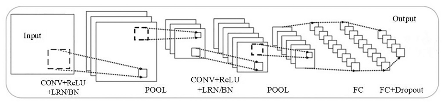
Illustration of a typical conventional neural network.

The generated feature maps usually have a considerable number of spatial dimensions after the convolutional operation. The pooling layer is added to reduce parameters, control over-fitting, and retain valid feature information. Convolution layers and pooling layers are repeated several times before being connected to the fully connected layers. In the fully connected layers, dropout layers randomly set input neurons as zero with a specific rate to avoid overfitting (Wu and Gu, 2015). In this research, CNN is employed to fuse the signals from multiple PWAS to signals from the conventional AE sensors. The framework of the proposed CNN-based multi-sensor data fusion will be described in Section 5.

2.3. Principal component analysis

Considering computational inefficiency for data analysis, principal component analysis (PCA) is one of the most popular multivariate statistical analyses. This method can transform high-dimensional data into a low-dimensional subspace while retaining the most important features of the original data (Abdi and Williams, 2010). During the dimensional reduction process of PCA, new relevant variables defined as principal components (PC) are generated. The cumulative contribution rate (CCR) is used to select the proper number of PCs which is expressed as:

CCR = \sum_{i = 1}^{k} D_{i} / \sum_{i = 1}^{N} D_{i}

(3)

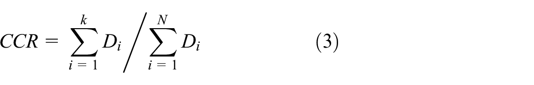
where D_i is the singular values of matrix Σ in decreasing order, representing the directions of the variances. The goal is to select the value of k to be as small as possible but with a reasonably high CCR. In the context of SHM, PCA has been extensively applied with the extracted features from AE signals in the time domain (Baccar and Söffker, 2017).

3. Experimental set-up

3.1. Sensors applied for measurements

Shape, material, and geometry are key parameters for selecting PWAS. PWAS disks are commonly used due to their omnidirectional Lamb wave generation and sensing capabilities (Sohn and Lee, 2010). Regarding the material selection, two material parameters are significant when selecting suitable PZT materials (Giurgiutiu and Zagrai, 2000), namely the piezoelectric charge coefficient d₃₁ and the piezoelectric voltage coefficient g₃₁. The design methodology of PWAS for actuators and receivers has been addressed in depth by Ochôa et al. (2019). Ochôa proposed using this formulation for the sensor output voltage V₀, which is directly proportional to the harmonic function f (ξ^S, ξ^A, r_a). This function accounts for the influence of sensor radius and frequency:

| V_{0} | \propto | r_{a} [\sum_{ξ^{S}} ξ^{S} J_{1} (ξ^{S} r_{a}) + \sum_{ξ^{A}} ξ^{A} J_{1} (ξ^{A} r_{a})] | = f (ξ^{S}, ξ^{A}, r_{a})

(4)

where r_a is the sensor radius, x^S and x^A are the wavenumbers of the symmetric and antisymmetric Lamb wave modes, respectively. The wavenumbers are dependent on frequency, as known as a dispersion relation. J₁ is the Bessel function of Order 1. Equation (4) allows the evaluation of the frequency sensitivity of thin PZT sensors as receivers under different radiuses.

Due to the electro-mechanical (E/M) behavior, the piezo ceramic may experience two extreme states, resonance, and anti-resonance. Typically, an unstable transitory regime can be formulated from the points of resonance and anti-resonance. This regime should be avoided as it is detrimental to the steady and reliable application of PZT sensors. Giurgiutiu proposed equations to calculate the admittance Y(w) and impedance Z(w) of a circular PZT sensor constrained by a structure (Giurgiutiu, 2007):

\begin{matrix} Y (w) = \\ iw \bar{C} {1 - k_{p}^{2} [1 - \frac{(1 + v_{a}) J_{1} (\bar{ϕ})}{\bar{ϕ} J_{0} (\bar{ϕ}) - [(1 - v_{a}) - \bar{χ} (w) (1 + v_{a})] J_{1} (\bar{ϕ})}]} \end{matrix}

(5)

\begin{matrix} Z (w) = Y^{- 1} (w) = \frac{1}{iw \bar{C}} \\ {1 - k_{p}^{2} [1 - \frac{(1 + v_{a}) J_{1} (\bar{ϕ})}{\bar{ϕ} J_{0} (\bar{ϕ}) - [(1 - v_{a}) - \bar{χ} (w) (1 + v_{a})] J_{1} (\bar{ϕ})}]}^{- 1} \end{matrix}

(6)

where C is the electrical capacitance of the thin PZT sensors, k_p is the complex planar electromechanical coupling coefficient of the PZT material, v_a is the Poisson ratio of the PZT material, J₁ and J₀ is the Bessel functions of Order 1 and Order 0, respectively. The complex phase angle in the PZT material is represented by $\bar{ϕ}$ = r_a·(w/ ${\bar{c}}_{a}$ ), where ${\bar{c}}_{a}$ is the complex in-plane wave speed in the PZT material and w is the angular frequency. The frequency-dependent complex stiffness ratio $\bar{χ}$ (w) is given by $\bar{χ}$ (w) = ${\bar{k}}_{str}$ (w)/ ${\bar{k}}_{PWAS}$ , where ${\bar{k}}_{str}$ (w) is the structural stiffness and ${\bar{k}}_{PWAS}$ is the stiffness of PZT sensors. The detailed calculation of the above unknown parameters can be found in (Giurgiutiu, 2007). It should be noted that structural vibrations are considered in this calculation method. The mechanical damping ratio h and the electrical damping ratio d are usually smaller than 5% for various thin PZT sensors. The zeros of the denominator of equation (5) represent the resonance points. The sensor thickness is considered in the E/M response, which allows the selection of the appropriate thickness for thin PZT sensors.

For the AE application, the criteria for employing PWAS only as receivers are proposed in (Cheng et al., 2022): (a) The selected PWAS must have a high piezoelectric voltage coefficient of g₃₁ and sufficient sensitivity over the frequency range for the intended application. For instance, The frequency range for metallic structures is recommended as 100–900 kHz (Ozevin, 2020); (b) The electro-mechanical (E/M) resonance point of the PWAS should not coincide with or be close to any local peaks in the PWAS voltage output. Additionally, at least one of these local peaks should fall within the investigated frequency range; (c) PWAS of greater thickness are preferred since their output response amplitudes are directly proportional to the thickness (Inman et al., 2005). Following these criteria, PZT-1 (r_a:10 mm × TH: 0.79 mm), PZT-2 (r_a:5 mm × TH: 0.8 mm), and PZT-3 (r_a:3 mm × TH: 0.5 mm) were selected ultimately. TH is the thickness of the PZT sensors.

The properties of the selected three types of PWAS are illustrated in Table 1 and Figure 7. Figure 8 displays the sensor output f (ξ^S, ξ^A, r_a) and E/M admittance response |Y| of PZT-1/2/3, which satisfy criteria (b). Frequencies beyond 500 kHz are removed because they are useless for the majority of applications (Ozevin, 2020). In the frequency band of interest, PZT-1 has multiple resonant frequencies compared to other sensors. The sensor output considering thickness f (ξ^S, ξ^A, r_a) × TH for PZT-1/2/3 is shown in Figure 8(d). It can be observed that these three PWAS together span a frequency range of 0–500 kHz efficiently, which is inaccessible to individual PWAS. For the R15α sensor and WSα sensor, their frequency sensitivity spectra are obtained from MISTRAS Group (Figure 9).

Table 1.

Characteristics of sensors.

Parameters	R15α	WSα	PZT-1	PZT-2	PZT-3
Weight (g)	34	32	1.90	0.49	0.18
r _a (mm)	9.5	9.5	10	5	3
TH (mm)	22.40	21.40	0.79	0.80	0.50
Material	PZT-5A (Boukabache et al., 2014)	PZT-5A	PIC155	PIC155	PIC255
g ₃₁ × 10⁻³ (Vm/N)	−12.4	−12.4	−12.9	−12.9	−11.3

r_a and TH is the radius and thickness of selected sensors, respectively.

Figure 7.

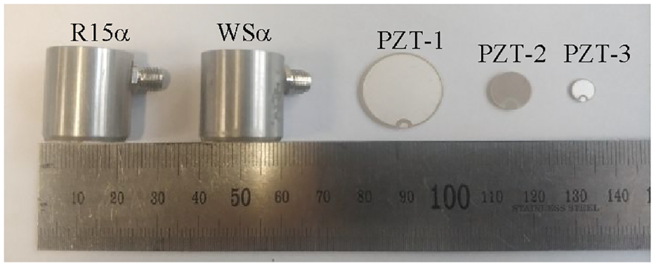
Illustration of the sensors used in the measurement.

Figure 8.

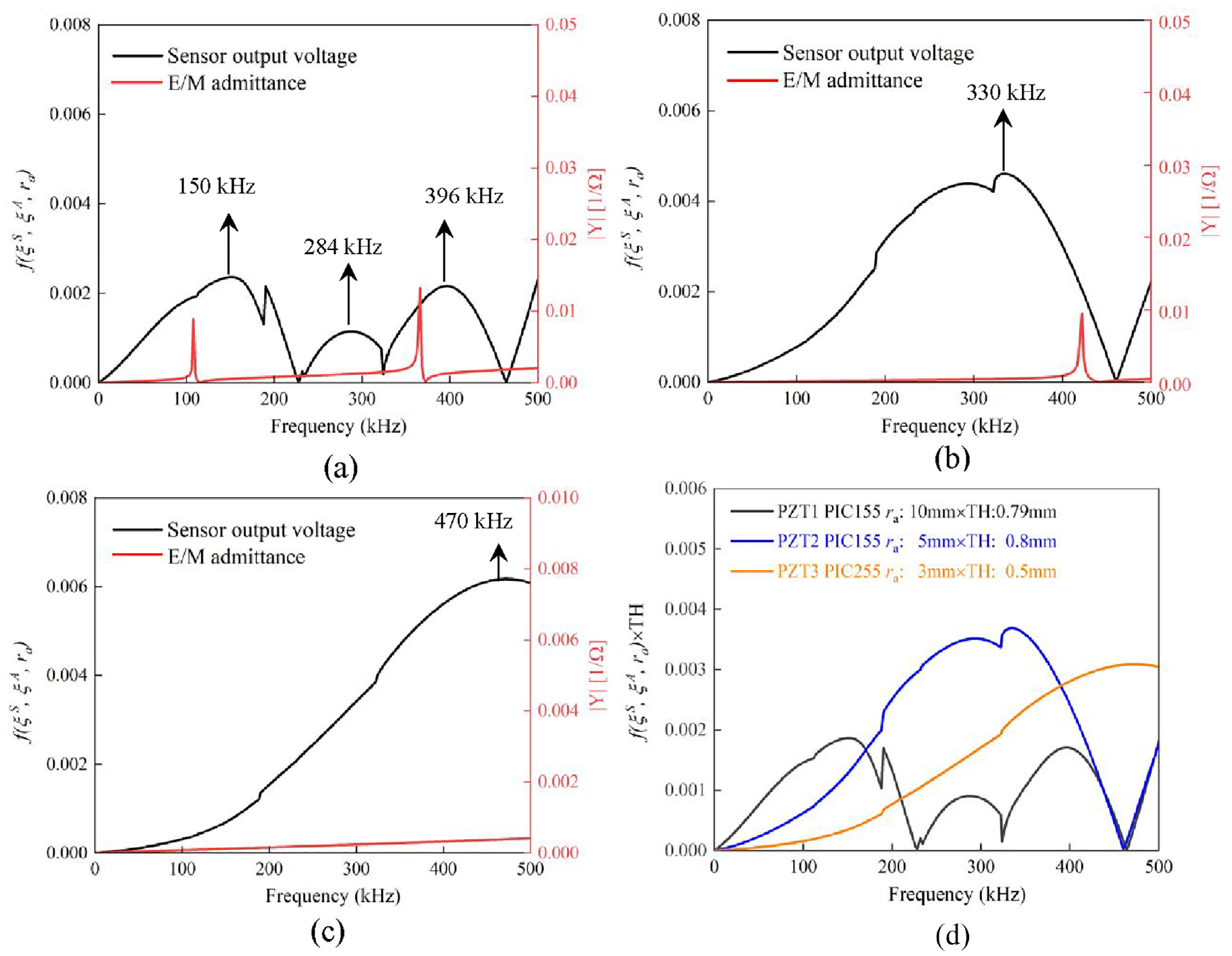
Sensor output f (ξ^S, ξ^A, r_a) and E/M admittance response of PZT-: (a) 1, (b) 2, (c) 3, and (d) frequency versus f (ξ^S, ξ^A, r_a) × TH for PZT-1/2/3.

Figure 9.

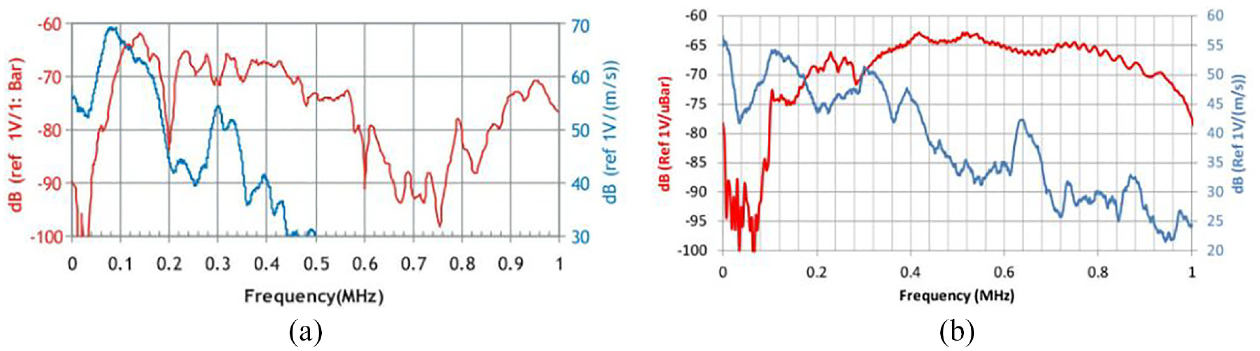
Frequency sensitivity spectrum of (a) R15α sensor, (b) WSα sensor.

3.2. Measurement setup

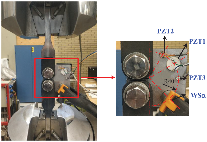
To assess the feasibility of PWAS of different sizes and to compare the results with those recorded using the conventional bulky AE sensors, compact tension (CT) specimens (85 mm length, 85 mm width, and 15 mm thickness), steel grade S355 were tested. The plate dimensions were selected such that the geometrical complexity and greater thickness are included in the measurements. Two sensor combinations were used in the tests (see Figure 10(a)): (1) R15α and PZT-1/2/3; and (2) WSα and PZT-1/2/3. To simulate the crack initiation, pencil lead breaking tests were performed at the notch tip (see Figure 10(b)). A total number of 120 pencil lead break tests were performed for each sensor layout while the parameters and settings remained the same for each test. To obtain enough data with randomness and uncertainty (Sause, 2011), the pencil leads were broken with various free lengths of 2–4 mm and contact angles of 20°–60°. The R15α sensor and WSα sensors were mounted on the specimen surface using a thin layer of silicone grease as an ultrasonic couplant. The PWAS were bonded to the specimen surface using cyanoacrylate glue.

Figure 10.

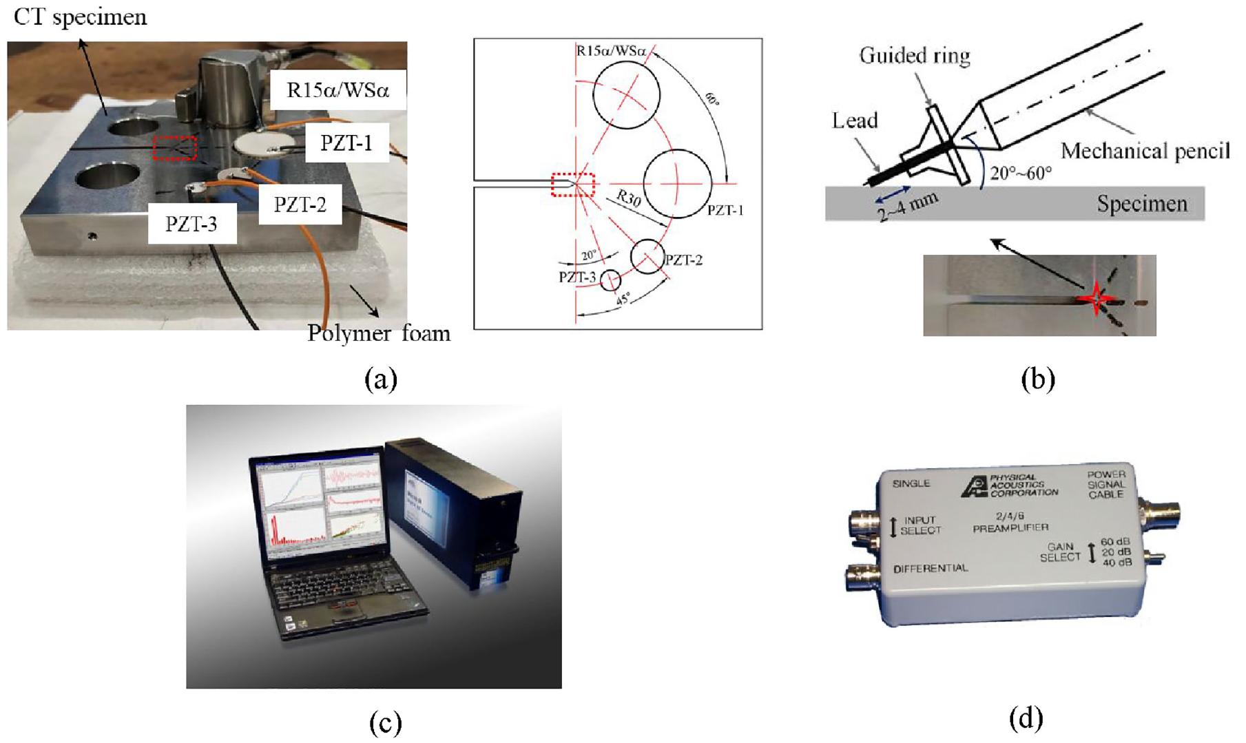
Experimental set-up: (a) layout of sensors, (b) illustration of PBL tests, (c) mistras AE system, (d) signal amplifier.

An eight-channel MISTRAS AE system with a 40 dB pre-amplifier was used. A threshold value of 50 dB was set to filter noise. Each measurement was recorded at a sampling rate of 5 MSPS (one sample per 0.2 μs) and 800 μs long. A pre-trigger of 256 μs was defined to capture the signal sources. The peak defined time (PDT), hit definite time (HDT), hit lookout time (HLT) and Max duration was set as 400, 800, 800, and 99 ms, respectively. These four timing parameters play significant roles in data acquisition, including hits recording and signal feature extraction. The definition of these timing parameters was determined using PBL trial tests.

4. Experimental results discussion

AE signals experience multiple reflections, refractions and mode conversion as a result of the geometrical complexity and dynamic environment (Cheng et al., 2021; Haile et al., 2018). During the PBL tests, background noise can be eliminated effectively by recording signals without loading. However, the AE hits caused by side-edge reflection and electronic noise cannot be completely avoided after breaking pencil leads. Hence, the recorded signals are separated into two categories: (a) the directly arrived hits as PBL signals; (b) other hits as noise signals. This section compares the PBL signals and noise signals recorded by chosen sensors. PBL signals measured from multi-sensors (in each layout) are identified using data association (Guel et al., 2020). An association is considered if the signals appear within a temporal window of less than 20 μs. This value was determined experimentally to ensure the accurate identification of the correct number of PBL events.

4.1. Signal response from breaking pencil leads

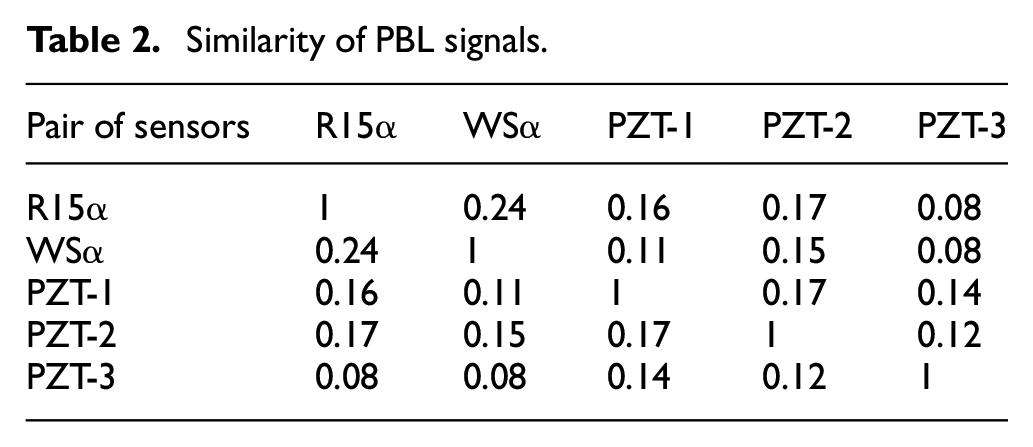
The similarity of PBL signals recorded from five types of sensors is analyzed using a cross-correlation coefficient (CCC) (Mukherjee and Banerjee, 2020). The higher value of CCC corresponds to the higher similarity between the signals from different pairs of sensors. The average values of the maximum cross-correlation coefficient (MCCC) obtained during 120 PBL events is summarized in Table 2. A low similarity between PBL signals from conventional AE sensors and PWAS (PZT-1/2/3) is observed in Table 2.

Table 2.

Similarity of PBL signals.

Pair of sensors	R15α	WSα	PZT-1	PZT-2	PZT-3
R15α	1	0.24	0.16	0.17	0.08
WSα	0.24	1	0.11	0.15	0.08
PZT-1	0.16	0.11	1	0.17	0.14
PZT-2	0.17	0.15	0.17	1	0.12
PZT-3	0.08	0.08	0.14	0.12	1

Examples of the waveform in the time domain, corresponding Continuous Wavelet Transform (CWT) scalogram, and FFT spectrum of PBL signals are shown in Figures 11 and 12. The CWT scalograms are employed to accurately discriminate the distribution of signal energy in both the time and frequency domains. The waveforms show significant differences and only PZT-3 exhibits a burst-type response. Differences are also strong in the CWT scalograms based on the Gabor wavelet of the waveforms as well. The aperture effect significantly distorts signals received by sensors with larger sizes, potentially introducing additional distortion from scattering or reflections (Tsangouri and Aggelis, 2018). Hence, PZT-3 shows a distinctive response that is less influenced by these distortions. The WSα sensor is characterized by a flat frequency response over a wideband frequency range of 100–1000 kHz. This sensor enables more accurate identification of the natural frequency characteristics of AE sources. The average value of PP_(80:500kHz) of 92% is calculated from the WSα sensor. Therefore, 80–500 kHz is selected as the primary frequency band of interest in the target objective.

Figure 11.

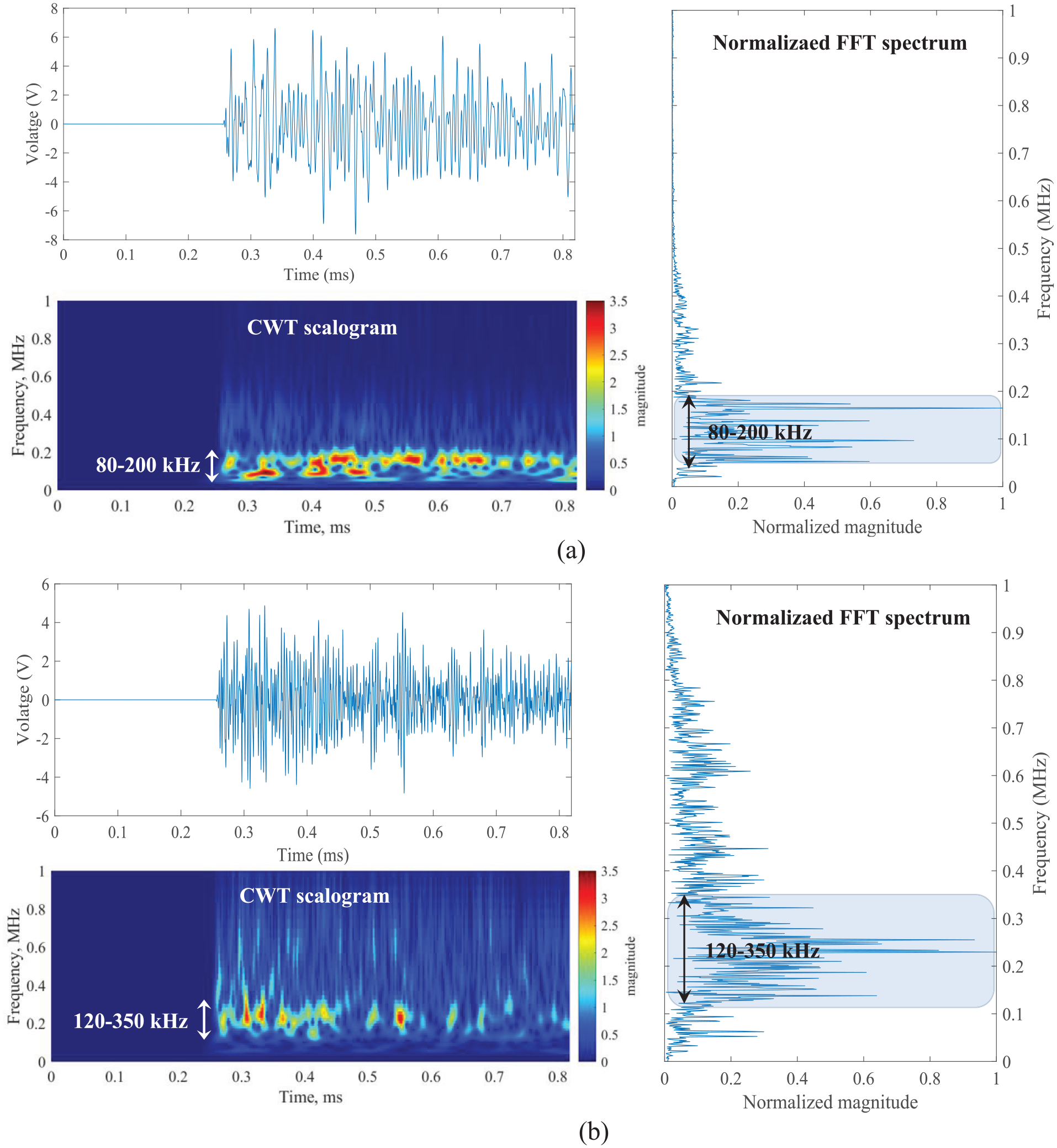
Example of AE signals captured by: (a) R15α sensor, (b) WSα sensor.

Figure 12.

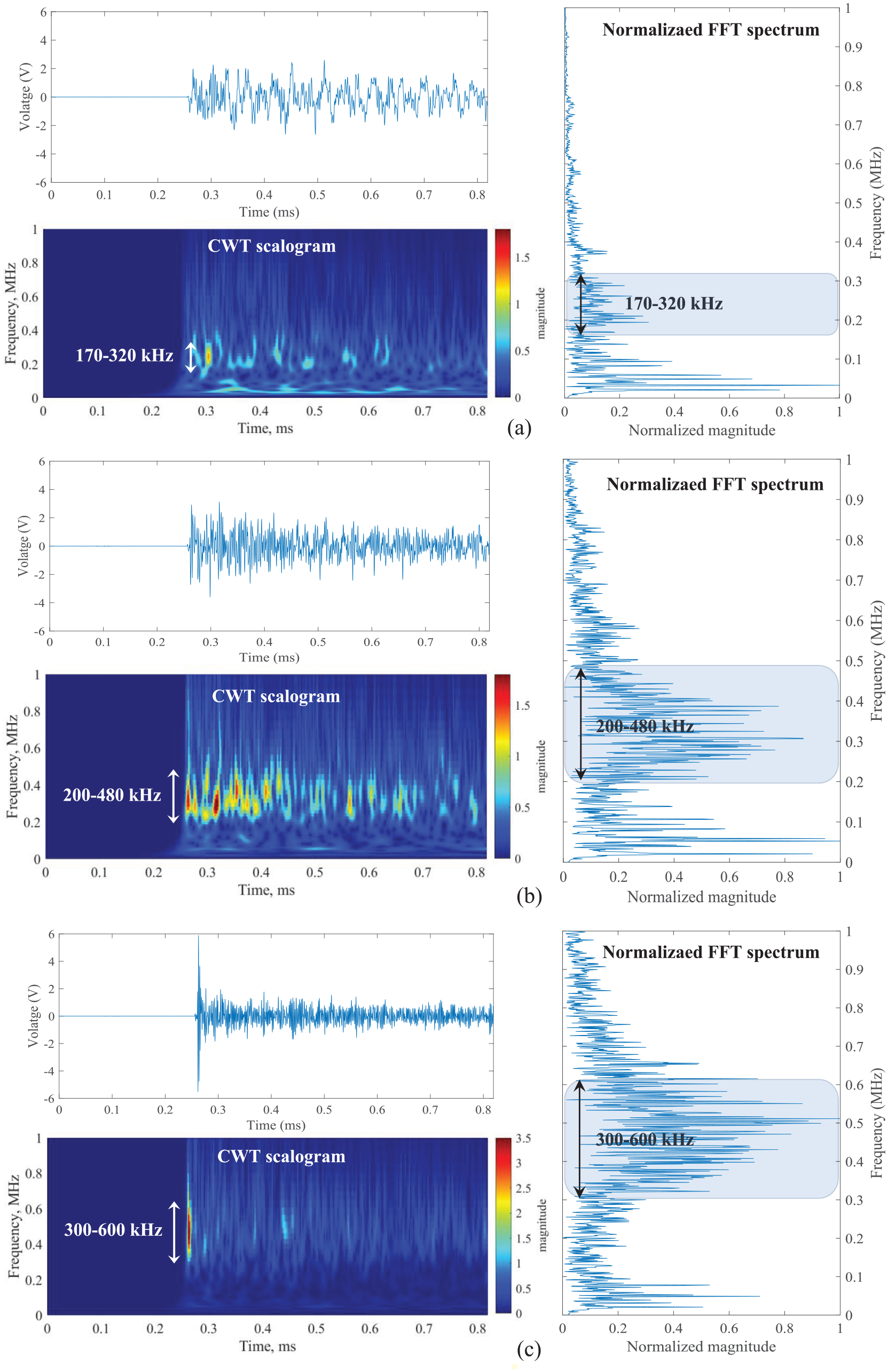
Example of AE signals captured by PZT-: (a) 1, (b) 2, and (c) 3.

Table 3 describes the properties of the signals obtained from various sensors as shown in Figures 11 and 12. The first row in Table 3 presents the resonant frequency of each sensor, as identified from their sensitivity responsese curves. Pertaining to PZT-1/2/3, the peaks of their sensor output function (see Figure 8) are extracted as the resonant frequency. The frequency band where sensors exhibit high sensitivity can be determined from the typical boundaries of areas with high intensity in the CWT scalograms from Figures 11 and 12. Comparing the sensitivity curves in Figure 8(d) with the high-sensitivity frequency bands listed in Table 3, it is noteworthy that the bands for PZT-2 and PZT-3 align well with the theoretical sensitivity response. However, for PZT-1, the frequency band with high sensitivity shifts relative to the theoretical curve due to its comparatively lower sensitivity. This shift also explains why the amplitude of the signal captured by PZT-1 is smaller than that of the other two PWAS. The frequency peak observed in the low-frequency range (below 100 kHz) in the FFT response shown in Figure 12 can be attributed to electromagnetic interference during measurement (Giurgiutiu and Zagrai, 2000). It is important to note that the theoretical sensitivity response curve assumes wave propagation through an infinite isotropic plate, which is not achievable in practice. Boundary effects interfere with wave propagation and even affect the first pulse received by the sensor. Consequently, the actual frequency response of the PBL signal differs from the theoretical curves.

Table 3.

Time dependency of the frequency content of signals from different sensors.

Characteristics	R15α	WSα	PZT1	PZT2	PZT3
Resonant frequency (kHz)	150	650	150/284/396	330	470
Frequency band with high sensitivity (kHz)	80–200	120–350	170–320	250–450	300–600
Overlap in amplitude distribution	No	No	Yes	Yes	Yes
Overlap in the frequency domain	Obviously	Partially	Obviously	Partially	Obviously

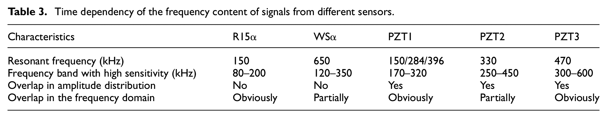
The WSα sensors clarify that the primary frequency composition of detected signals is between 120 and 350 kHz, which is the original feature of the AE source. However, the R15α sensor drastically changes its frequency content to 80–200 kHz. Similarly, the frequency sensitivity of PWAS also affects the nature of the AE-emitted source (see the second row in Table 3). The significant attenuation of the signal captured by PZT-3 can be ascribed to the fact that the nature frequency of detected signals deviates from its high resonant frequency.

4.2. Signal distinction

Compared to other features, the amplitude of signals is independent of the acquisition threshold (Santo et al., 2019). The amplitude distribution of recorded signals during the PBL tests is shown in Figure 13 to quantify the uncertainty of recorded signals. As seen in Figure 13, the R15α sensor presents a much higher amplitude compared to the other sensors, representing a higher sensitivity. The median values of amplitude from the other sensors are approximately similar to each other. Noise signals can be distinguished effectively by considering the amplitude of the signals. The amplitude of PBL signals captured by R15α and WSα usually exceeds 88 dB. Signal association techniques [35] are employed to distinguish PBL signals from noise signals for PZT-1/2/3. The conventional bulky AE sensors show a more reliable performance than PWAS without overlap of amplitude distribution between PBL and noise signals. The fourth row in Table 3 presents the overlap in amplitude distribution of sensors.

Figure 13.

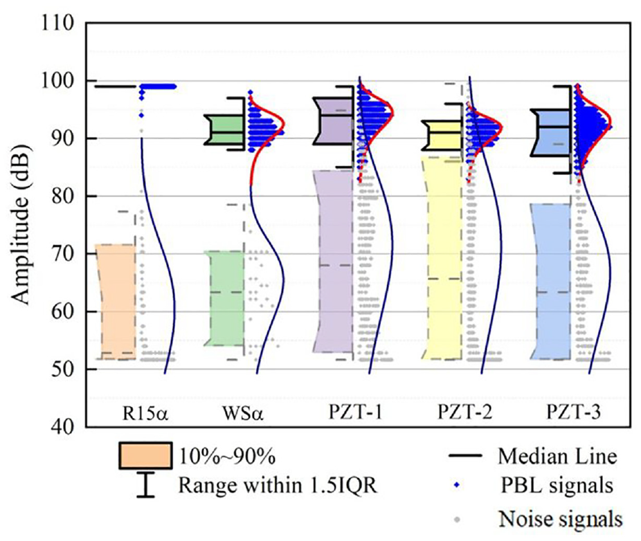
Amplitude distribution of PBL signals and noise signals captured by the investigated sensors.

The distinction between signals from PBL and noise is necessary to guarantee the sensor performance for damage detection. As seen in Figure 14, the WSα sensor captures the smallest number of noise signals compared to other sensors. In contrast, it can be observed that the other sensors record a significant amount of noise signals that are not the first arrived signals. This indicates that the WSα sensor offers superior data quality compared to the other sensors, highlighting its enhanced performance in capturing the desired signals. Figure 15 shows the comparison between signals recorded by different types of sensors in the frequency domain. The PBL signals recorded by R15α, PZT-1, and PZT-3 clearly overlap with the noise signals in the frequency domain. On the contrary, the noise signals from WSα and PZT-2 can be efficiently filtered by high-pass and low-pass filtering with a narrow overlap band, respectively. The situation of overlap in the frequency domain between recorded PBL and noise signals is summarized in Table 3. Considering that the R15α sensor is more sensitive to noise than WSα, WSα shows a performance benefit in AE detection, especially in a noisy environment.

Figure 14.

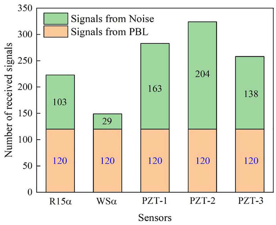
Number of received signals during PBL tests.

Figure 15.

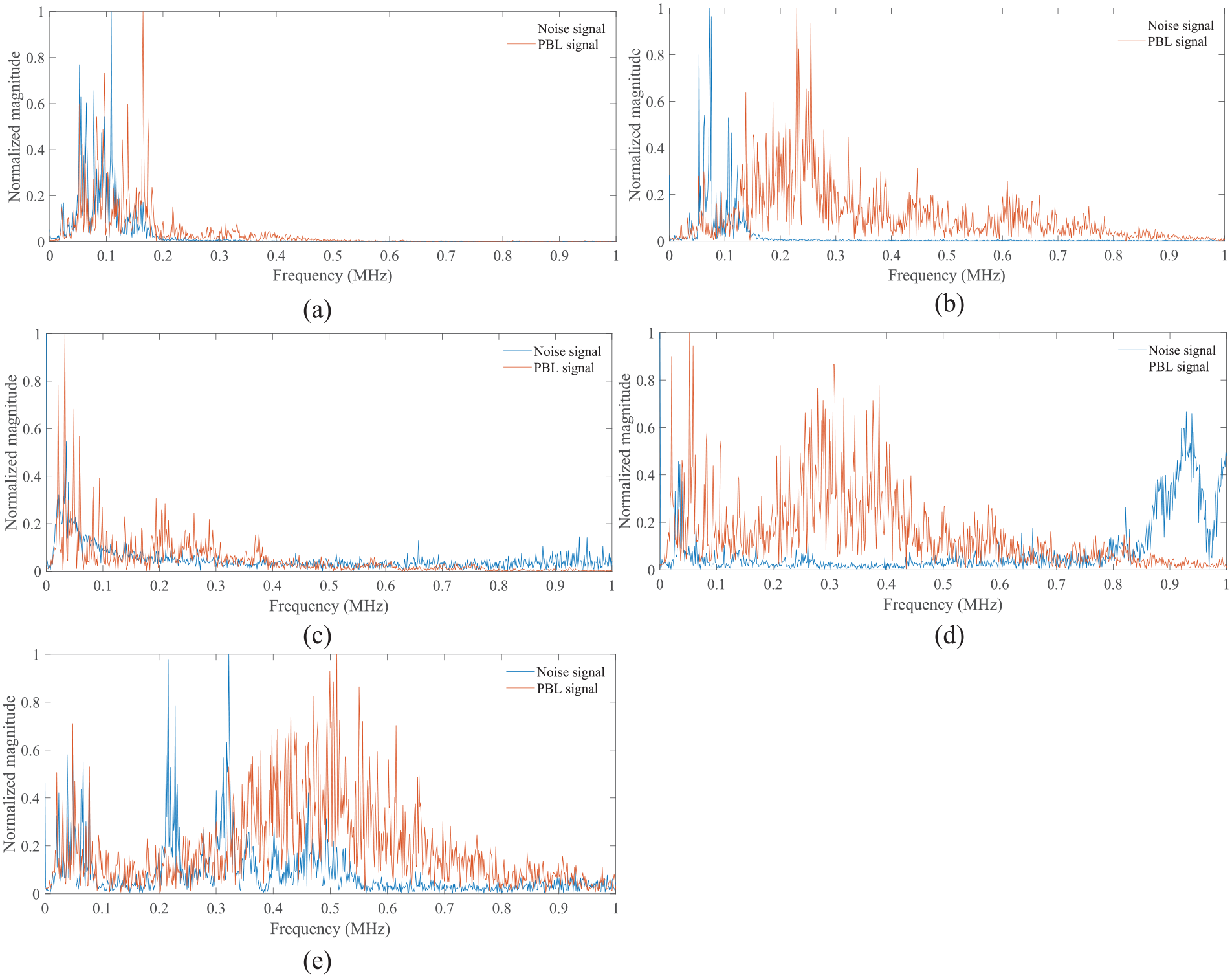
Comparison of signals from: (a) R15α, (b) WSα, (c) PZT-1, (d) PZT-2, and (e) PZT-3.

5. Data fusion of multiple PWAS

As described in Section 4, the WSα sensor is an attractive option for AE detection in a noisy situation. To extend the application of PWAS in fatigue monitoring of structures, this section proposes the methodology to fuse the data from multiple PWAS to WSα sensors.

5.1. Data preparation

The experimental set-up for the fatigue test is presented in Figure 16. PBL tests were manually performed at the notch tip of the installed CT specimens, using a measurement set-up similar to that described in Section 3.2. To account for variations in bonding layer and soldering quality, four CT specimens equipped with PWAS sensors were tested to collect data. In this set-up, pencil leads were broken from both sides of the specimens to represent the actual crack initiation. In total, 5484 pairs of PBL signals were captured using data association. The signals captured by PWAS are prepared as the input data, while the output is the signals received by WSα sensor.

Figure 16.

Experimental set-up for data fusion.

To increase the computational efficiency, the signals used for data fusion are pre-processed in the following steps: (1) remove pre-trigger of 256 μs; (2) cut waveform to a certain wavelength of 200 μs to make sure a satisfactory frequency resolution of 5 kHz; (3) remove the electrical noise that contaminates the signals through the implementation of appropriate filters 80–500 kHz; (4) PCA is applied to reduce the number of features as seen in Figure 17, which makes the machine learning model simpler and less data hungry. It should be noted that PCA is employed for the signals both from the PWAS and the WSα. PCA is conducted with the open-source Python package scikitlearn.

Figure 17.

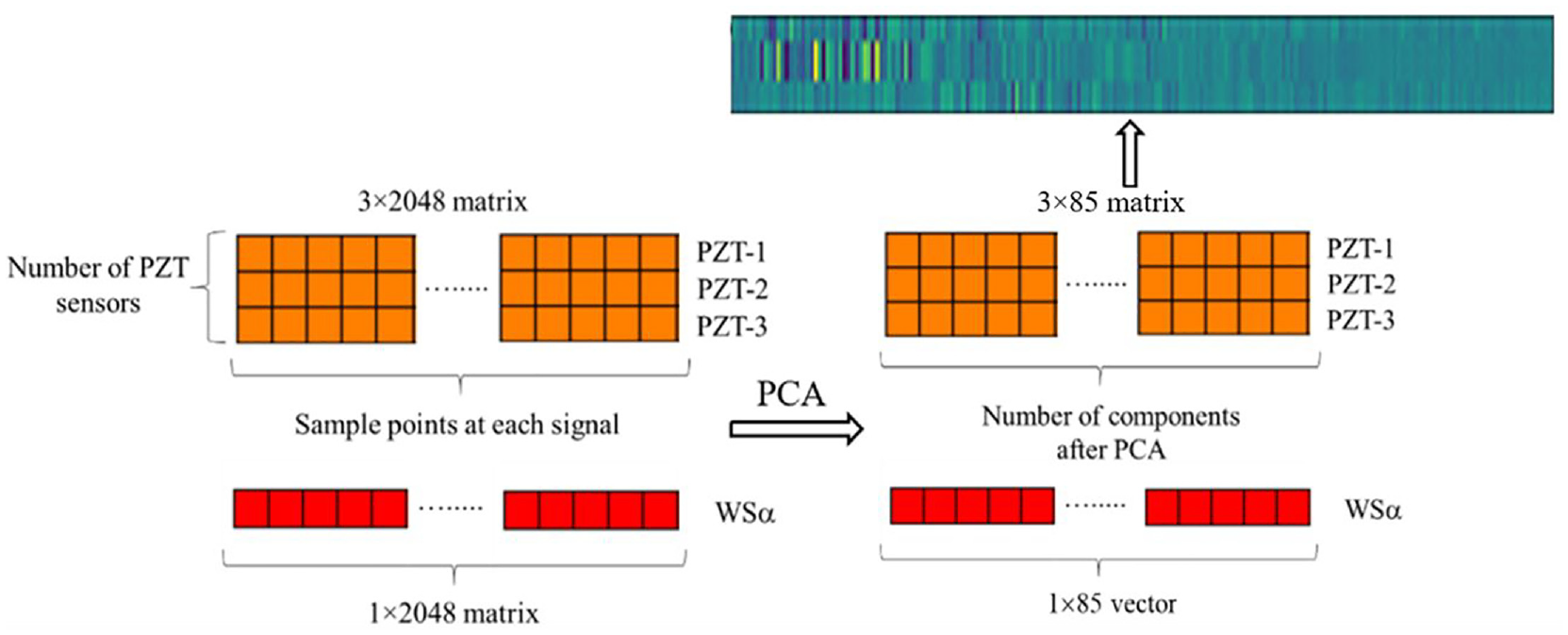
Preparation of database by PCA.

The cumulative contribution rate (CCR) of the first 85 principal components (PCs) is described in Figure 18(a). CCR increases accordingly as the number of employed PCs increases and reaches around 95% with k = 85. This indicates that most information in the waveforms is represented by the first part of the PCs. Hence, it is determined that PCA is efficient to compress the feature number from 2048 to 85 with only a 5% loss of the total information in the original waveforms. Figure 18(b) shows an example to illustrate the comparison between original waveforms and PCA-inversed waveforms. After that, the reduced 3 × 85 matrix of 5484 events is saved as images as shown in Figure 17. These images are then passed as the input data for the CNN model in this research. The corresponding dimension of output data is also decreased from 2048 to a vector with 85 features.

Figure 18.

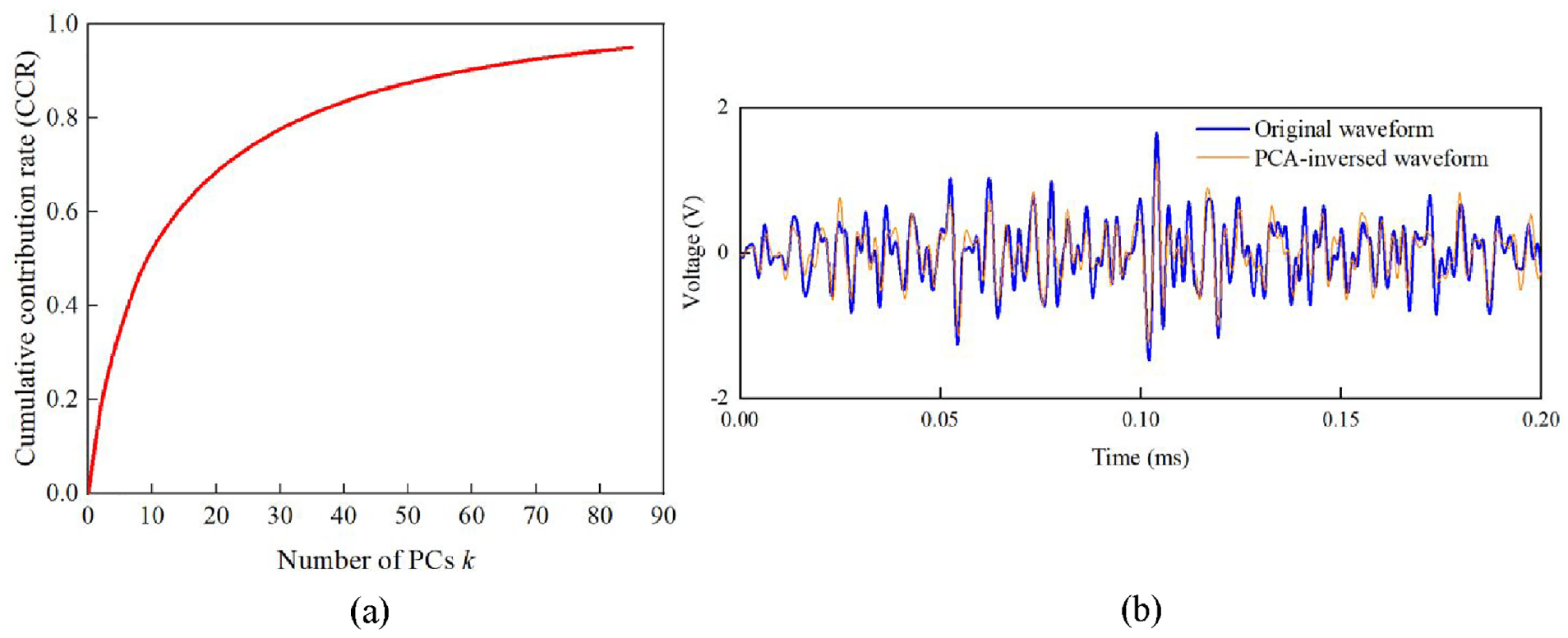
(a) The contribution rate for the first 85 principal components, (b) comparison between original and PCA inversed waveforms.

5.2. Customized model evolution

The contribution rate of each principal component is represented by the PCA singular value D_i. To signify the uneven contribution of features in the CNN model, a weighted Mean Squared Error (MSE) is utilized (Chang et al., 2022) as the loss function. PCs with higher contribution rates are weighted more heavily than those with low contribution rates:

Weighted MSE = \sum_{i = 1}^{n} \sum_{j = 1}^{r} \frac{λ_{i}}{\sum_{k = 1}^{85} λ_{k}} (y_{i, j} - y_{i, j}')^{2}

(7)

The i-th sample’s actual and predicted values in the j-th feature are represented by y _i,j and $y_{i, j}'$ , respectively. ${\bar{y}}_{j}'$ is the average result of the j-th calculations. The CNN model is capable of being trained and evaluated with information about the different importance of PCs using the adjusted MSE.

The cross-correlation function is commonly used to evaluate the similarity between time series (Cassisi et al., 2012). Hence, the averaged MCCC between actual and predicted value after PCA-inverse is calculated as the assessment indicator.

Accuracy = \frac{1}{n} \sum_{i = 1}^{n} MCCC (Y_{i}, Y_{i}^{'})

(8)

The i-th sample’s actual and predicted values after PCA-inverse transformation are represented by Y_i and $Y_{i}^{'}$ , respectively.

5.3. CNN model construction

The developed model is named N_AE-PZT, which means that it is a “Network trained to fuse the output from PWAS for AE monitoring.” N_AE-PZT adopts the waveform information from PWAS as input values. Similar to a typical CNN model, the input is transformed into a more and more abstract and composite representation layer by layer. Finally, the signal from the conventional bulky AE sensor is reconstructed.

N_AE-PZT is a fully convolutional neural network as shown in Figure 19. The first layer is the input layer of 3 × 85 × 3 pixels resolutions. The input layer receives images representing the signals from three types of PWAS, and then these images are fed into two Conv blocks. Each Conv block contains two Conv layers with ReLU as an activation function and a Batch Normalization (BN) layer. In the second Conv block, a Maximum Pooling (MaxPool) layer is added to reduce the number of features. Ultimately, the feature maps are flattened into a single 1 × 85 vector via a Global Average Pooling (GAPool) layer and a Fully Connected (FC) layer.

Figure 19.

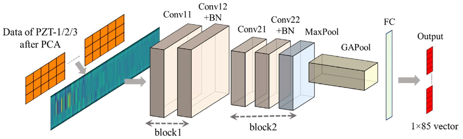
Architecture of the proposed model N_AE-PZT.

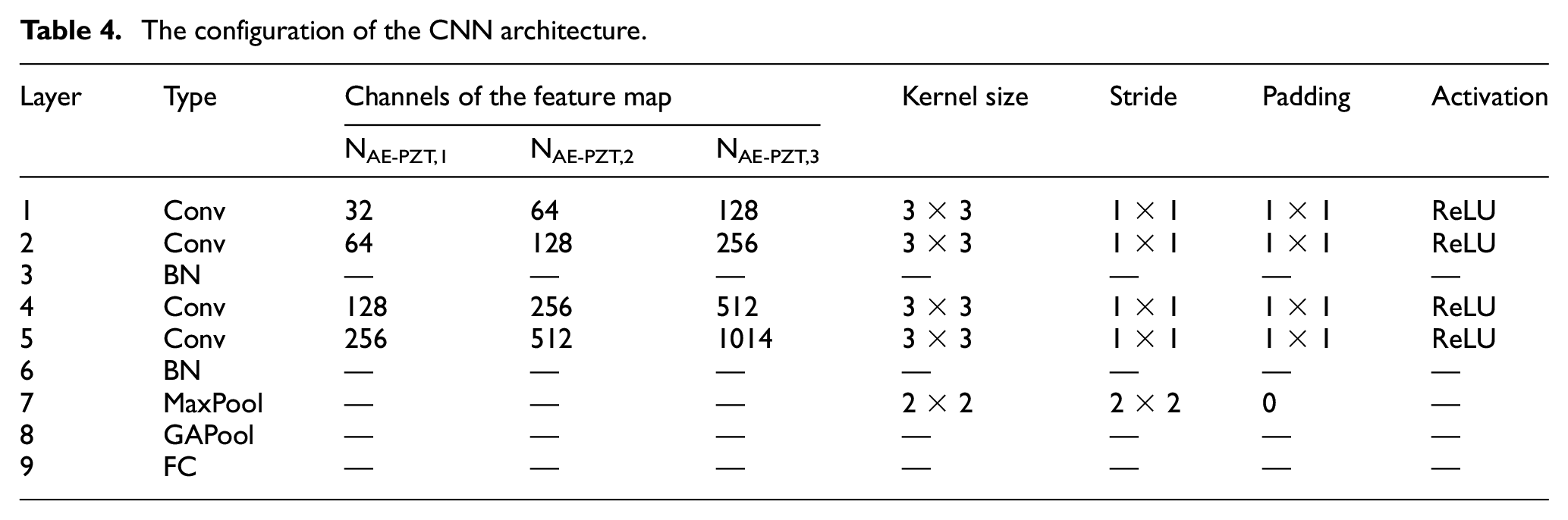
Three kinds of CNNs with identical layers and different channels of feature maps are adopted which are named N_AE-PZT,1, N_AE-PZT,2, and N_AE-PZT,3 respectively. The detailed network settings are given in Table 4. During the convolution operation, the kernel size is selected as 3 × 3 by considering the real input size and processing time.

Table 4.

The configuration of the CNN architecture.

Layer	Type	Channels of the feature map			Kernel size	Stride	Padding	Activation
		N_AE-PZT,1	N_AE-PZT,2	N_AE-PZT,3
1	Conv	32	64	128	3 × 3	1 × 1	1 × 1	ReLU
2	Conv	64	128	256	3 × 3	1 × 1	1 × 1	ReLU
3	BN	—	—	—	—	—	—	—
4	Conv	128	256	512	3 × 3	1 × 1	1 × 1	ReLU
5	Conv	256	512	1014	3 × 3	1 × 1	1 × 1	ReLU
6	BN	—	—	—	—	—	—	—
7	MaxPool	—	—	—	2 × 2	2 × 2	0	—
8	GAPool	—	—	—	—	—	—	—
9	FC	—	—	—	—	—	—	—

5.4. CNN model training

The dataset as described in Section 5.1 is imported into the constructed CNN architecture. A comparison study of three kinds of CNNs was performed to investigate the influence of the complexity of the network. The CNN model adopts a split dataset in a ratio of 4:1 because of the relatively small dataset. Thus, there are 4935 and 549 samples in the training and testing datasets, respectively. Testing data is not used for training the network. A batch size equal to 32 was adopted with a shuffling approach to redistribute the data for better performance. This CNN model was built and trained with a learning rate of 0.001 in PyTorch.

5.5. Evaluation of the trained CNN

Figure 20 illustrates the training history of loss and learning curves of three models for the training and testing dataset. The loss and accuracy values are shown in every one epoch and the maximum number of epochs employed in this research is 500. The accuracy represents the difference between the actual and predicted waveforms from the associated WSα sensor. The increasing rate of training accuracy is very fast at the beginning of the training process. Afterwards, the value of loss and accuracy becomes steady. The final accuracy of three CNNs is above 95% for training data. The final testing accuracy of N_{AE_PZT1}, N_{AE_PZT2}, and N_{AE_PZT3} reaches 76%, 79%, and 82%, respectively. Under identical layers, N_{AE_PZT3} delivers the best prediction performance which was selected for further analysis.

Figure 20.

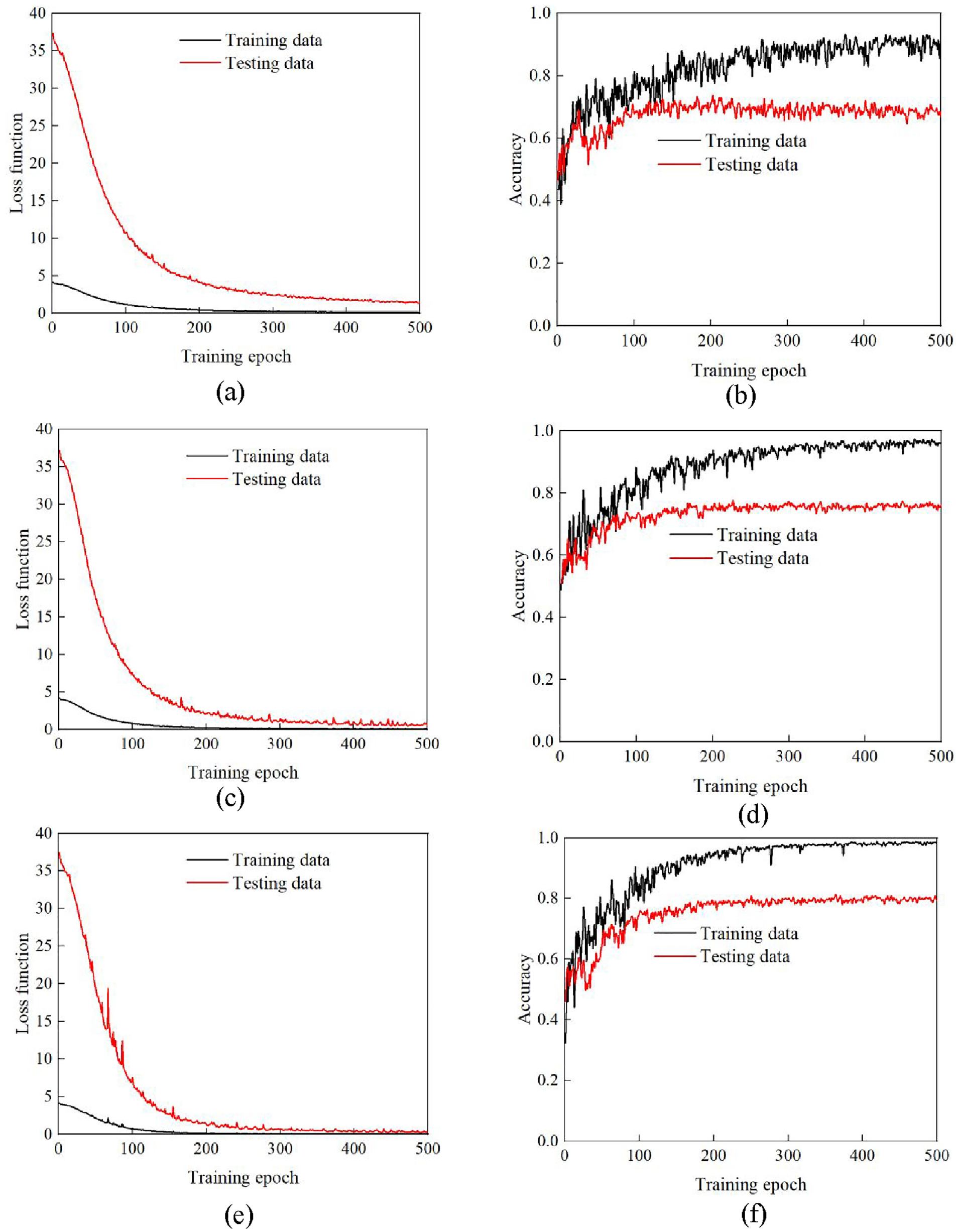
(a) Loss and (b) learning curves of N_{AE_PZT1}, (c) loss and (d) learning curves of N_{AE_PZT2}, (e) loss and (f) learning curves of N_{AE_PZT3}.

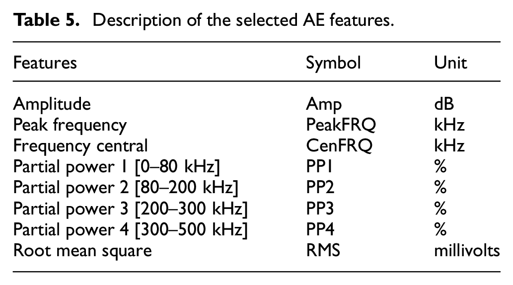
The relative frequency of MCCC between actual and predicted results is calculated to show the percentage of samples with high prediction accuracy. As shown in Figure 21 (bottom-left corner), the MCCC values for 99% of the training dataset and 86% of the testing dataset of N_{AE_PZT3} were found to be higher than 0.8. This indicates that 14% of the testing dataset fails to be reconstructed with high accuracy. To further evaluate the reliability of the N_{AE_PZT3}, the AE features listed in Table 5 are extracted from the actual and predicted waveforms for comparison. These features are extracted as they are slightly threshold-dependent (Santo et al., 2019) and have been applied effectively for damage identification (Kharrat et al., 2016; Sause et al., 2012; Vetrone et al., 2021; Wisner et al., 2019). Figure 21 shows the correlation matrix of AE features from actual and predicted results. The average value of the correlation coefficients for the training data and testing data are 93% and 74%, respectively. It should be noted that the correlation value of the peak frequency is relatively lower than the other features. This can be attributed to the characteristics of the wide-band frequency response of the WSα sensor.

Figure 21.

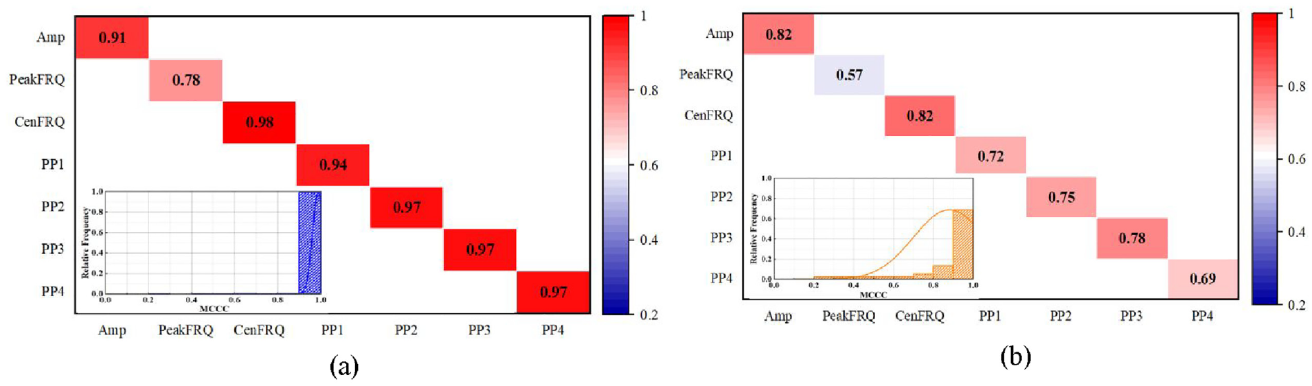
Feature correlation matrix and MCCC between actual and predicted results of (a) training dataset, (b) testing dataset.

Table 5.

Description of the selected AE features.

Features	Symbol	Unit
Amplitude	Amp	dB
Peak frequency	PeakFRQ	kHz
Frequency central	CenFRQ	kHz
Partial power 1 [0–80 kHz]	PP1	%
Partial power 2 [80–200 kHz]	PP2	%
Partial power 3 [200–300 kHz]	PP3	%
Partial power 4 [300–500 kHz]	PP4	%
Root mean square	RMS	millivolts

Mean absolute deviation (MAD) quantifies the spread in the dataset. It is computed as the average of the absolute differences between each data point and the mean value. A smaller MAD represents a dataset that is more clustered. After calculation, it was found that the peak frequency of the actual waveforms from the WSα sensor has the highest MAD of 0.13, while the MAD values of the other features are less than 0.09. This demonstrates that peak frequency is more widespread and less effective for identification and classification. Hence, Figure 22 presents the distributions of the parameters with high feature correlation values except for the peak frequency. By comparison, the distribution of these parameters predicted by N_{AE_PZT3} closely coincides with the distribution of actual results in the testing dataset. These results further justify that the proposed network model N_{AE_PZT3} can effectively reconstruct the waveforms from the reference sensor.

Figure 22.

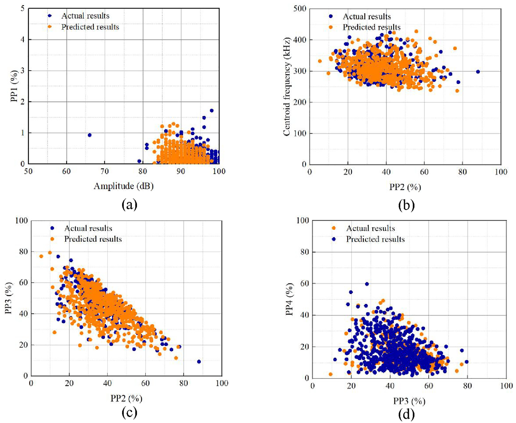
Distributions of AE parameters extracted from actual and predicted results.

5.6. Further discussion

It can be concluded that the proposed methodology achieves high precision and reliability for data-level fusion using multi-PWAS. As the feature indication of damage-related signals of WSα is well reconstructed and identified, the damage detection can be performed after successful data fusion of multiple PWAS. However, it should be underlined that this proposed methodology is validated using PBL tests on CT specimens, which are less challenging compared to real practical situations.

It should be noticed that this data fusion methodology is validated using a dataset where sensors are placed at a uniform distance from the source. In future works, the uncertainties caused by different sensor layouts, measuring cables, and soldiering qualities should be considered to train the CNN. For example, this study does not consider variations in distance between the source and each PWAS. Moreover, fatigue tests are imperative to the development and validation of the proposed approach. This method could be particularly useful for identifying the formation of crack tips. Crack propagation can alter wave propagation characteristics and potentially limit the effectiveness of this method. A comparative study of deep learning methods and architectures is also recommended to improve the accuracy of damage detection using PWAS. Last but not least, future studies should explore the field applications of the proposed method to different types of structures with restricted-access areas, especially thicker/complex structures. Such studies are expected to shed new light on possible improvements in the performance of PWAS in AE monitoring. In the future, we will continue to work in this direction, and we hope that other scientists interested in SHM will share data sets to encourage progress in the field.

6. Conclusion

To enhance the functionality of PWAS-based AE application, this paper presents a methodology for performing a data-level fusion of outputs from various PWAS. The performance of selected PWAS is compared to bulky AE sensors, which are widely used for SHM in several fields. After identifying the advantages of the WSα sensor, the reconstruction of the signal measured via WSα was successfully achieved by fusing the signals from multiple PWAS using a developed CNN model N_AE-PZT. The key findings are summarized as follows:

(1) The feasibility of the selected PWAS is identified using PBL tests. The chosen three PWAS are found to be more effective in covering the frequency range than an individual PWAS. According to the comparative analysis performed for sensors response captured from breaking pencil leads test on the CT specimens, the R15α sensor and PWAS alter the original features of the AE-emitted source dramatically, while WSα sensor represents the nature of the AE source with higher fidelity due to its flat and wideband frequency response function.

(2) Compared to other types of sensors, the WSα sensor captures the smallest number of noise signals during PBL tests. Besides, the signal response of WSα sensor shows a slight overlap in amplitude and frequency content distribution between PBL and noise signals. Thus, WSα sensor is an attractive option concerning the clear distinction between signals from PBL and noise.

(3) 5484 PBL events were used to train and evaluate the performance of the three developed CNNs with different architectures. All the CNNs can deliver convincing prediction performance in reconstructing the waveforms from the reference sensor, with accuracy all above 95% for training data. N_AE-PZT,3 reaches satisfying accuracy for testing data than the other two models.

(4) Feature correlation analysis and similarity analysis are carried out for all datasets. The distribution patterns of seven AE parameters with high feature correlation values predicted by N_AE-PZT,3 is found to be consistent with the actual results. As a result, the proposed method shows the promising application potential to enable damage detection using multi-PWAS combing with a waveform-based data-fusion method.

Abbreviations

The following abbreviations are used in this manuscript:

SHM Structural health monitoring

NDT Non-destructive testing

AE Acoustic emission

PWAS Piezoelectric wafer active sensors

SNR Signal-to-noise ratio

PBL Pencil break lead

CNNs Convolutional neural networks

PCA Principal component analysis

OWT Offshore wind turbine

CT Compact tension

ANNs Artificial neural networks

ReLU Rectified linear unit

LRN Local response normalization

BN Batch normalization

PDT Peak defined time

HDT Hit definite time

HLT Hit lookout time

Footnotes

Acknowledgements

The first author wishes to express her gratitude for the financial support of the China Scholarship Council (CSC) under grant number 201806060122. Dr. Ali Nokhbatolfoghahai is supported by the AIRTuB project (Automatic Inspection and Repair of Turbine Blades), funded with a Top Sector Energy subsidy from the Ministry of Economic Affairs of the Netherlands.

Credit author statement

Lu Cheng: Conceptualization, Methodology, Software, Validation, Formal analysis, Investigation, Writing Original draft, Visualization. Ali Nokhbatolfoghahai: Conceptualization, Validation, Supervision, Writing - Review& Editing. Roger Groves: Conceptualization, Supervision, Writing - Review & Editing. Milan Veljkovic: Conceptualization, Supervision, Writing - Review & Editing.

Declaration of conflicting interests

The authors declared no potential conflicts of interest with respect to the research, authorship, and/or publication of this article.

Funding

The authors received no financial support for the research, authorship, and/or publication of this article.

ORCID iD

Ali Nokhbatolfoghahai

Data availability statement

The data supporting the findings of this study are available from the corresponding author upon reasonable request.

References

Abdi

Williams

(2010) Principal component analysis. Wiley Interdisciplinary Reviews: Computational Statistics 2(4): 433–459.

Alom

Taha

Yakopcic

, et al. (2019) A state-of-the-art survey on deep learning theory and architectures. Electronics 8(3): 292.

Baccar

Söffker

(2017) Identification and classification of failure modes in laminated composites by using a multivariate statistical analysis of wavelet coefficients. Mechanical Systems and Signal Processing 96: 77–87.

Barile

Casavola

Pappalettera

, et al. (2020) Application of different acoustic emission descriptors in damage assessment of fiber reinforced plastics: A comprehensive review. Engineering Fracture Mechanics 235: 107083.

Bhuiyan

Lin

Giurgiutiu

(2018) Acoustic emission sensor effect and waveform evolution during fatigue crack growth in thin metallic plate. Original Article Journal of Intelligent Material Systems and Structures 29(7): 1275–1284.

Boukabache

Escriba

Fourniols

J-Y

(2014) Toward smart aerospace structures: Design of a piezoelectric sensor and its analog interface for flaw detection. Sensors 14(11): 20543–20561.

Broer

Galanopoulos

Benedictus

, et al. (2021) Fusion-based damage diagnostics for stiffened composite panels. Structural Health Monitoring 21(2): 613–639.

Calabrese

Proverbio

(2020) A review on the applications of acoustic emission technique in the study of stress corrosion cracking. Corrosion and Materials Degradation 2(1): 1–30.

Carrasco

Méndez

Leaman

, et al. (2021) Short review of the use of acoustic emissions for detection and monitoring of cracks. Acoustics Australia 49(2): 273–280.

10.

Cassisi

Montalto

Aliotta

, et al. (2012) Similarity measures and dimensionality reduction techniques for time series data mining. In: Karahoca

(ed.) Advances in Data Mining Knowledge Discovery and Applications. London: InTech, pp.71–96.

11.

Chang

Wan

, et al. (2022) Convolutional neural network for predicting crack pattern and stress-crack width curve of air-void structure in 3D printed concrete. Engineering Fracture Mechanics 271: 108624.

12.

Chen

Zhou

, et al. (2020) An acoustic-homologous transfer learning approach for acoustic emission–based rail condition evaluation. Structural Health Monitoring 20(4): 2161–2181.

13.

Cheng

Nokhbatolfoghahai

Groves

, et al. (2022) Acoustic emission-based detection in restricted-access areas using multiple PZT disc sensors. In: European workshop on structural health monitoring, Palermo, Italy, pp. 619–629.

14.

Cheng

Xin

Groves

, et al. (2021) Acoustic emission source location using Lamb wave propagation simulation and artificial neural network for I-shaped steel girder. Construction and Building Materials 273: 121706.

15.

Creusen

KEY

Misios

Winkes

, et al. (2022) Introducing the C1 wedge connection. Steel Construction 15(1): 13–25.

16.

Dehghan Niri

Farhidzadeh

Salamone

(2013) Adaptive multisensor data fusion for acoustic emission (AE) source localization in noisy environment. Structural Health Monitoring 12(1): 59–77.

17.

ElBatanouny

Abdelrahman

Ziehl

(2014) Review of acoustic emission corrosion monitoring of prestressed Concrete bridges. In: PCI convention and national bridge conference, Washington, DC.

18.

Giurgiutiu

(2007) Structural Health Monitoring with Piezoelectric Wafer Active Sensors. Amsterdam, The Netherlands: Elsevier.

19.

Giurgiutiu

(2020) Structural health monitoring (SHM) of aerospace composites. In: Irving

Soutis

(eds) Polymer Composites in the Aerospace Industry. UK: Elsevier – Woodhead Pub, pp.491–558.

20.

Giurgiutiu

Zagrai

(2000) Characterization of piezoelectric wafer active sensors. Journal of Intelligent Material Systems and Structures 11(12): 959–976.

21.

Godin

Reynaud

Fantozzi

(2018) Challenges and limitations in the identification of acoustic emission signature of damage mechanisms in composites materials. Applied Sciences 8(8): 1267.

22.

Gomez

AEA

(2017) Development MEMS acoustic emission sensors. Thesis, University of South Florida.

23.

Grosse

Ohtsu

Aggelis

, et al. (eds) (2008) Acoustic Emission Testing: Basics for Research–Applications in Engineering. Verlag Berlin Heidelberg: Springer Nature.

24.

Guel

Hamam

Godin

, et al. (2020) Data merging of AE sensors with different frequency resolution for the detection and identification of damage in oxide-based ceramic matrix composites. Materials 13(20): 4691.

25.

Haile

Bordick

Riddick

(2018) Distributed acoustic emission sensing for large complex air structures. Structural Health Monitoring 17(3): 624–634.

26.

Hamam

Godin

Fusco

, et al. (2019) Modelling of acoustic emission signals due to fiber break in a model composite carbon/epoxy: Experimental validation and parametric study. Applied Sciences 9(23): 5124.

27.

Meng

, et al. (2021) An overview of acoustic emission inspection and monitoring technology in the key components of renewable energy systems. Mechanical Systems and Signal Processing 148: 107146.

28.

Inman

Farrar

Junior

, et al. (eds) (2005) Damage Prognosis: For Aerospace, Civil and Mechanical Systems. Hoboken, NJ: John Wiley & Sons.

29.

Jiang

Zhang

Wang

, et al. (2018) Monitoring fatigue damage of modular bridge expansion joints using piezoceramic transducers. Sensors 18(11): 3973.

30.

Joseph

Mei

Migot

, et al. (2021) Crack-length estimation for structural health monitoring using the high-frequency resonances excited by the energy release during fatigue-crack growth. Sensors 21(12): 4221.

31.

Kharrat

Ramasso

Placet

, et al. (2016) A signal processing approach for enhanced Acoustic Emission data analysis in high activity systems: Application to organic matrix composites. Mechanical Systems and Signal Processing 70–71: 1038–1055.

32.

Le Gall

Monnier

Fusco

, et al. (2018) Towards quantitative acoustic emission by finite element modelling: Contribution of modal analysis and identification of pertinent descriptors. Applied Sciences 8(12): 2557.

33.

Liu

Yao

Zhang

, et al. (2020) Multi-sensor data fusion for remaining useful life prediction of machining tools by iabc-bpnn in dry milling operations. Sensors 20(17): 4657.

34.

Liu

Yang

Zio

, et al. (2018) Artificial intelligence for fault diagnosis of rotating machinery: A review. Mechanical Systems and Signal Processing 108: 33–47.

35.

Mukherjee

Banerjee

(2020) Analysis of acoustic emission signal for crack detection and distance measurement on steel structure. Acoustics Australia 49(1): 133–149.

36.

Nair

Cai

(2010) Acoustic emission monitoring of bridges: Review and case studies. Engineering Structures 32(6): 1704–1714.

37.

Nakamura

(2016) Practical Acoustic Emission Testing. Japan: Springer.

38.

Nokhbatolfoghahai

Navazi

H. M

Groves

R. M.

(2022). Use of dictionary learning for damage localization in complex structures. Mechanical Systems and Signal Processing, 180, 109394.

39.

Ochôa

Groves

Benedictus

(2019) Systematic multiparameter design methodology for an ultrasonic health monitoring system for full-scale composite aircraft primary structures. Structural Control and Health Monitoring 26(5): e2340.

40.

Ozevin

(2020) MEMS acoustic emission sensors. Applied Sciences 10(24): 8966.

41.

Saboonchi

Ozevin

Kabir

(2016) MEMS sensor fusion: Acoustic emission and strain. Sensors and Actuators A: Physical 247: 566–578.

42.

Saeedifar

Zarouchas

(2020) Damage characterization of laminated composites using acoustic emission: A review. Composites Part B: Engineering 195: 108039.

43.

Santo

Sattar

Edwards

(2019) Validation of acoustic emission waveform entropy as a damage identification feature. Applied Sciences 9(19): 4070.

44.

Sause

(2011) Investigation of pencil-lead breaks as acoustic emission sources. Journal of Acoustic Emission 29: 184–196.

45.

Sause

MGR

Gribov

Unwin

, et al. (2012) Pattern recognition approach to identify natural clusters of acoustic emission signals. Pattern Recognition Letters 33(1): 17–23.

46.

Sohn

Lee

(2010) Lamb wave tuning curve calibration for surface-bonded piezoelectric transducers. Smart Materials and Structures 19(1): 015007.

47.

Trujillo

Zagrai

Meisner

, et al. (2014) Monitoring of acoustic emission activity using thin wafer piezoelectric sensors. In: Proceedings volume 9064, health monitoring of structural and biological systems 2014, San Diego, CA, vol. 906418, pp.360–371. SPIE.

48.

Tsangouri

Aggelis

(2018) The influence of sensor size on acoustic emission waveforms—a numerical study. Applied Sciences 8(2): 168.

49.

Verstrynge

Lacidogna

Accornero

, et al. (2021) A review on acoustic emission monitoring for damage detection in masonry structures. Construction and Building Materials 268: 121089.

50.

Vetrone

Obregon

Indacochea

, et al. (2021) The characterization of deformation stage of metals using acoustic emission combined with nonlinear ultrasonics. Measurement 178: 109407.

51.

Wisner

Mazur

Perumal

, et al. (2019) Acoustic emission signal processing framework to identify fracture in aluminum alloys. Engineering Fracture Mechanics 210: 367–380.

52.

Wotzka

Cichoń

(2020) Study on the influence of measuring AE sensor type on the effectiveness of OLTC defect classification. Sensors 20(11): 3095.

53.

(2015) Towards dropout training for convolutional neural networks. Neural Networks 71: 1–10.

54.

Jahanshahi

(2018) Data fusion approaches for structural health monitoring and system identification: Past, present, and future. Structural Health Monitoring 19(2): 552–586.

55.

Yang

Liu

, et al. (2018) A comparison of 1-D and 2-D deep convolutional neural networks in ECG classification. arXiv preprint arXiv:1810.07088.

56.

Xin

Cheng

Diender

, et al. (2020) Fracture acoustic emission signals identification of stay cables in bridge engineering application using deep transfer learning and wavelet analysis. Advances in Bridge Engineering 1(1): 1–16.

57.

Ziehl

Matta

, et al. (2013) Acoustic emission detection of fatigue damage in cruciform welded joints. Journal of Constructional Steel Research 86: 85–91.

58.

Momeni

Godinez

, et al. (2011) Adaptation of PWAS transducers to acoustic emission sensors. In: Proceedings volume 7983, nondestructive characterization for composite materials, aerospace engineering, civil infrastructure, and homeland security 2011, San Diego, CA, vol. 7983, pp.658–667. SPIE.

59.

Momeni

Godinez

, et al. (2012) Dual mode sensing with low-profile piezoelectric thin wafer sensors for steel bridge crack detection and diagnosis. Advances in Civil Engineering 2012: 402179.

60.

Zhang

Liu

, et al. (2020) Tension monitoring of wedge connection using piezoceramic transducers and wavelet packet analysis method. Sensors 20(2): 364.

Data level fusion of acoustic emission sensors using deep learning

Abstract

Keywords

1. Introduction

2. Overview of theoretical background

2.1. Acoustic emission signal features

2.2. Convolution neural network

2.3. Principal component analysis

3. Experimental set-up

3.1. Sensors applied for measurements

3.2. Measurement setup

4. Experimental results discussion

4.1. Signal response from breaking pencil leads

4.2. Signal distinction

5. Data fusion of multiple PWAS

5.1. Data preparation

5.2. Customized model evolution

5.3. CNN model construction

5.4. CNN model training

5.5. Evaluation of the trained CNN

5.6. Further discussion

6. Conclusion

Abbreviations

Footnotes

Acknowledgements

Credit author statement

Declaration of conflicting interests

Funding

ORCID iD

Data availability statement

References