
Abstract
Mathematical modeling of multilayered piezoelectric (PE) ceramic substantially acquires attention due to its distinctive advantages of fast response time, positioning, optical systems, vibration feedback, and sensors, such as deformation and vibration control. As such, fundamental solution of a PE structure is essential. This paper presents three-dimensional (3D) static and dynamic solutions (i.e. Green’s functions) in a multilayered transversally isotropic (TI) PE layered half-space. The uniform vertical mechanical load, vertical electrical displacement, and horizontal mechanical load are applied on the surface of the structure. The novel Fourier-Bessel series (FBS) system of vector functions (which is computationally more powerful and streamlined) and the dual-variable and position (DVP) method are employed to solve the related boundary-value problem. Two systems of first-order ordinary differential equations (i.e. the LM- and N-types) are obtained in terms of the FBS system of vector functions, with these expansion coefficients being the Love numbers. A recursive relation for the expansion coefficients is established by using DVP method that facilitates the combination of two neighboring layers into a new one and minimizes the computational effort to a great extent. The corresponding physical-domain solutions are acquired by applying the appropriate boundary/interface conditions. Several numerical examples pertaining to static and dynamic response are solved, and the efficiency and accuracy of the proposed solutions are validated with the existing results for the reduced cases. The solutions provided could be beneficial to better developments of PE materials, configurations, fabrication, and applications in the future.
Keywords
1. Introduction
Due to the intrinsic mechanical-electrical coupling effect, piezoelectric (PE) materials stimulate an abundance of interdisciplinary research (Azizi et al., 2016). Developing PE materials with structural systems like advanced composite beams, plates, and shells have enormous applications in emerging fields such as aerospace industries (Gasbarri et al., 2014), military operation (Barrett-Gonzalez and Wolf, 2022), and energy harvesting (Elahi et al., 2019). The designed smart structures include the shape control of large space antennas, active or passive control of vibration (Rao and Sunar, 1994; Yoon and Washington, 1998), miniature positioning devices, for example, micro-robots, medical apparatus, micro-pumps (Muralt et al., 1986), highly efficient micro-machined acoustic devices like microphones and micro speakers (Williams et al., 2012), hearing aids (Zargarpour and Zarifi, 2015), and chemical and biomedical ones (Huang and Lee, 2008; Manbachi and Cobbold, 2011). Recently, extensive studies are conducted on improving PE-based devices by utilizing the coupled electromechanical properties of PE materials (Cao and Yang, 2012; Gao and Zhang, 2020; Li et al., 2017; Yang et al., 2013).
Since the electric and mechanical fields are coupled together, there are many challenges associated with piezo-based devices where precise control of the electric field, mechanical stress, and the potential is needed. As such, various rigorous mathematical models are developed. For instance, Wang et al. (2002) acquired a state-vector method for the axisymmetric deformation in multilayered PE media. Three-dimensional Green’s functions in anisotropic tri-materials were studied by Yang and Pan (2002). Li et al. (2002) studied the stress singularities in PE-bonded structures. Pan (2003) presented a general method for deriving the Green’s functions in three-dimensional (3D) anisotropic PE and multilayered media. With the help of the extended Stroh formalism and two-dimensional (2D) Fourier transforms, Yang et al. (2004) investigated the 3D response in a multilayered anisotropic PE structure under the action of a point force and a point charge. Simplified models under different loading conditions and medium variable parameters were developed extensively to simulate the behavior of the PE structure in the past few decades (Chanda et al., 2023; Liew et al., 2003; Lu et al., 2018; Xiang and Shi, 2009; Zhang and Ma, 2015; Zhang et al., 2019; Zhou et al., 2017).
Various methods in modeling and simulation of the multilayered structure were proposed. These include the exact spectral elements method (Abad and Rouzegar, 2017), the finite element method (Hegendörfer et al., 2022), the space-time backward substitution method (Zhang et al., 2022), the dual reciprocity method (DRM) (Zhan et al., 2023), the meshless boundary element (Power et al., 2017), and the Stroh formalism method (Pan et al., 2023). In dealing with layering, the propagator matrix method (PMM) (Pan and Han, 2004), stiffness matrix method (Wang et al., 2022), precise integration matrix method (PIM) (Zhang et al., 2016), generalized reflection–transmission matrices method (Liu et al., 2020), the wave refraction method (Rafiee-Dehkharghani et al., 2021), the analytic layer-element method (Ai et al., 2022), and the reverberation-ray matrix method (Pao et al., 2007) were proposed.
Inspired by the PIM method, a new method named the dual-variable and position method (DVP) was recently proposed (Liu and Pan, 2018; Liu et al., 2018). This new method is much more advanced to address the time-dependent problem in various isotropic and transversally isotropic (TI) materials.
In this paper, we apply the DVP method along with the Fourier-Bessel series (FBS) system (Pan et al., 2021) to solve the time-harmonic response of TI layered PE half-spaces induced by a surface load or surface electric displacement. While the DVP method is unconditionally stable, the FBS system is much efficient than the traditional integral transform. The reason is that the FBS system only needs simple summation over the discrete zero points of the Bessel functions, whilst, in the integral transform method, numerical integration has to be carried out over each interval between these zero points (i.e. Liu et al., 2016; Moshtagh et al., 2017). Furthermore, since the expansion coefficients are discrete in terms of the FBS system, they can be served as Love numbers which can be saved and repeatedly used later for the calculation of the corresponding Green’s functions (i.e. Zhou et al., 2023). These Love numbers are derived and used to find the response/Green’s function in three typical layered structures proposed in this paper. The accuracy is validated by comparing with existing solutions. Numerical examples indicate the strong dependence of the time-harmonic responses on the input frequency, material layering, and loading types.
2. Description of the boundary-value problem
A multilayered transversally isotropic piezoelectric (TI-PE) structure composed of n different layers over a TI-PE half-space is considered in this paper as shown in Figure 1. A global cylindrical coordinate system (r, θ, z) is introduced in such a way that the (r, θ)-plane is on the surface and the layered half-space is in the positive z-direction. Layer j is bounded by the interfaces z = zj and z = zj−1 with a thickness of hj = zj−zj−1. Without losing the generalization, we assume that a uniform time-harmonic load is applied within a circular region of radius
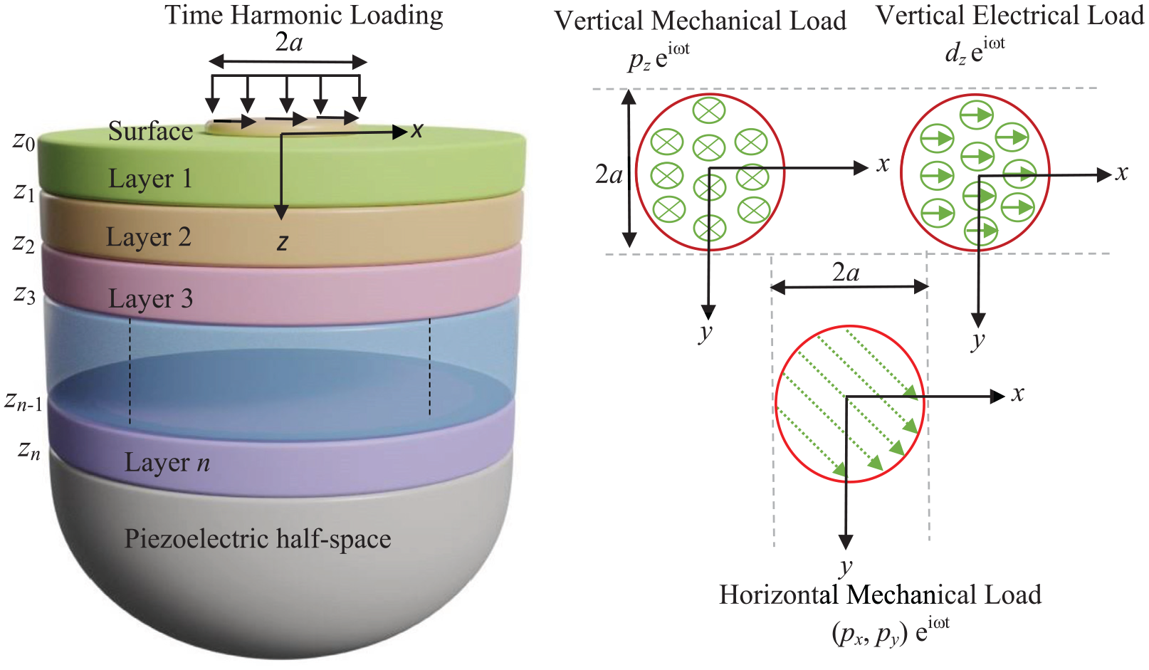
A TI-PE layered half-space under time-harmonic loads (in both vertical direction along z-axis and horizontal direction in the (x, y)-plane) within a circle of radius a on the surface.
2.1. Fundamental equations
In terms of the cylindrical coordinates, the time-harmonic wave equation for the PE material without body force and body charge (i.e. proportional to eiωt) is given by
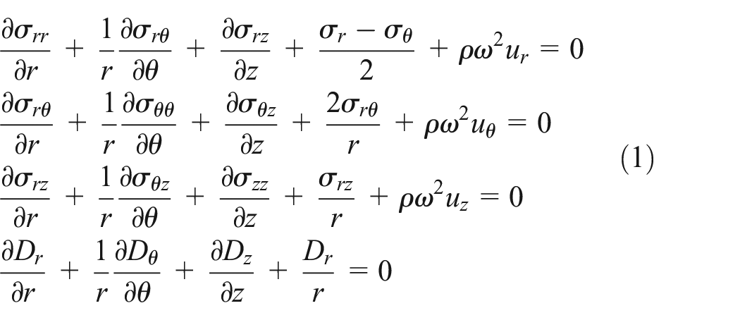
where σ ij (N/m2) (i, j = r, θ, z), Dj (C/m2), ρ (kg/m3), ui (m), and ω = 2πf (f (Hz = 1/s)) are the stress, electric displacement, mass density, elastic displacement, and angular frequency.
The linear constitutive relation for the TI-PE material (with its symmetry axis along z-axis) in the cylindrical coordinate system is given by
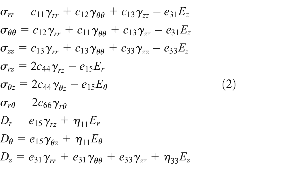
where cij (N/m2), eij (C/m2), and η ij (C2/N m2) are the elastic constant tensor, PE constant tensor, and dielectric coefficients tensor, respectively; γ ij (dimensionless) and Ei (V/m) are the strain and electric field; c66 = 0.5 (c11−c12) for the TI material.
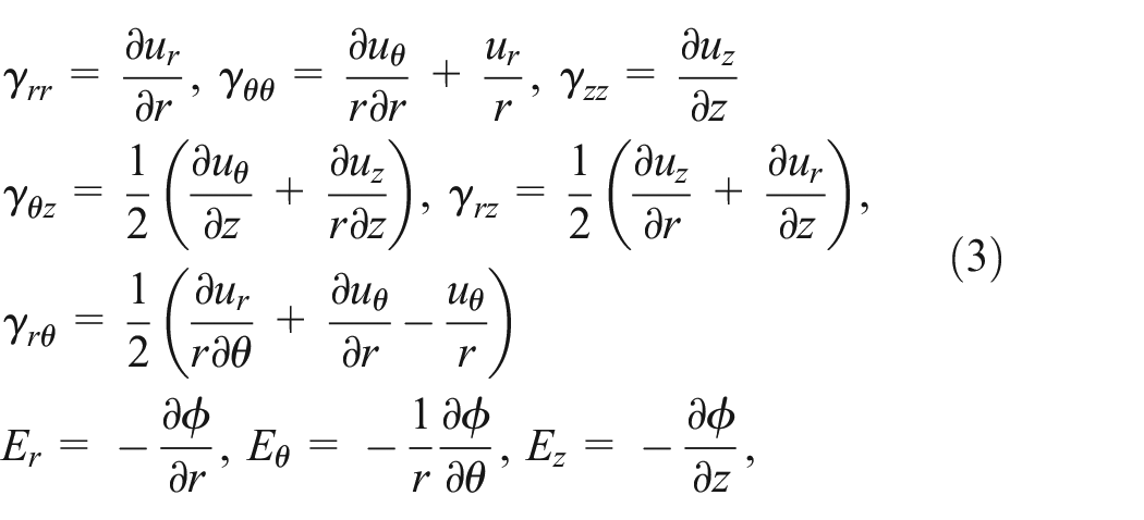
The strain components γ ij and electrical field Ej can be expressed in terms of mechanical displacements ui and electric potential φ (V) as
2.2. Boundary and interface conditions
2.2.1. Condition on the surface
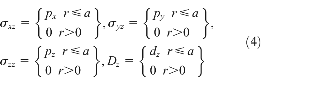
It is assumed that, on the surface z = z0, a uniform load of time-harmonic is applied within the circle of radius a as shown in Figure 1. Then, the boundary condition at z = z0 (=0) (in term of Cartesian coordinate system, and proportional to eiωt) is given by
2.2.2. Continuity condition at any interface z = zk (except for the half-space)
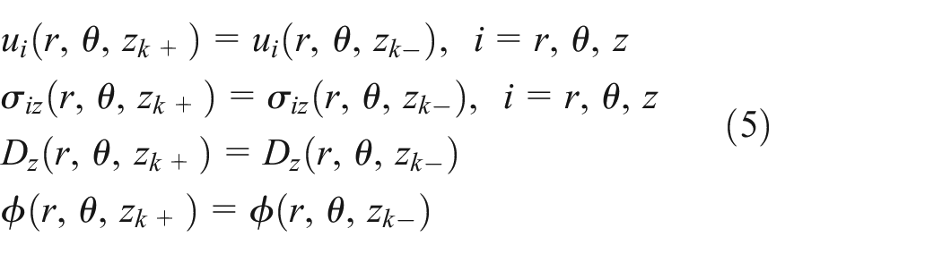
It is assumed that the interface is perfectly bonded. Namely, the mechanical displacements, tractions, electrical displacements, and electric potential are continuous across it, for example, at z = zk,
In the last homogeneous TI-PE half-space, we require that the solution there is finite. In other words, the elastic displacements and electric potential are zero when z approaches infinity. This condition will be restated later.
3. Fundamental solution in term of the new vector system and the DVP method
3.1. Fourier-Bessel series system of vector functions
To solve the problem, the powerful FBS system of vector functions is introduced (Pan et al., 2021)
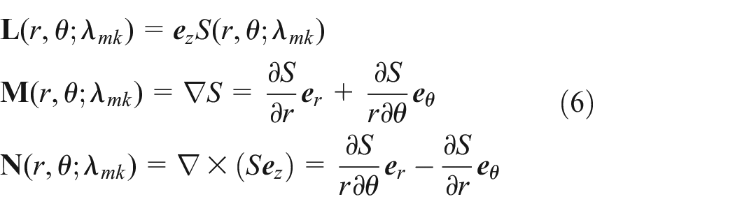
where
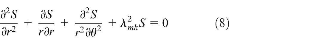
The scalar function in equation (6) is given by
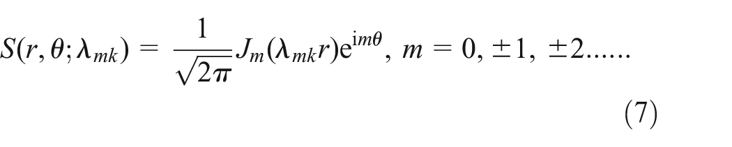
which is a solution of the Helmholtz equation
It is worthy to mention that the FBS system of vector function is motivated by the spectral element method where the approximation is made in the physical domain by truncating the radial distance at a large R. This novel approach is fundamentally different from the traditional Hankel integral transform where approximation is made in the transformed wavenumber domain (Pan et al., 2021). Due to the orthogonality of FBS system (equation (6)), the displacement vector (
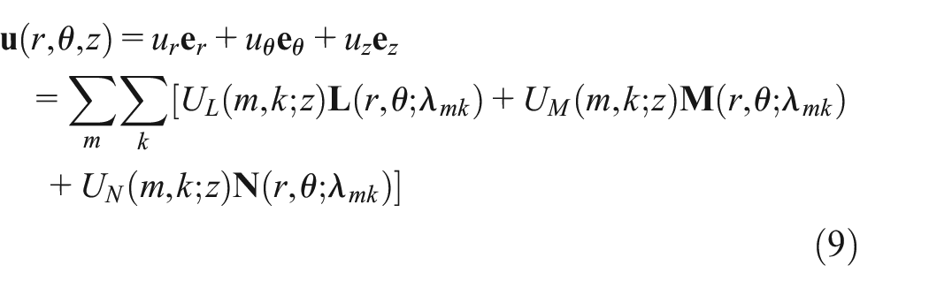
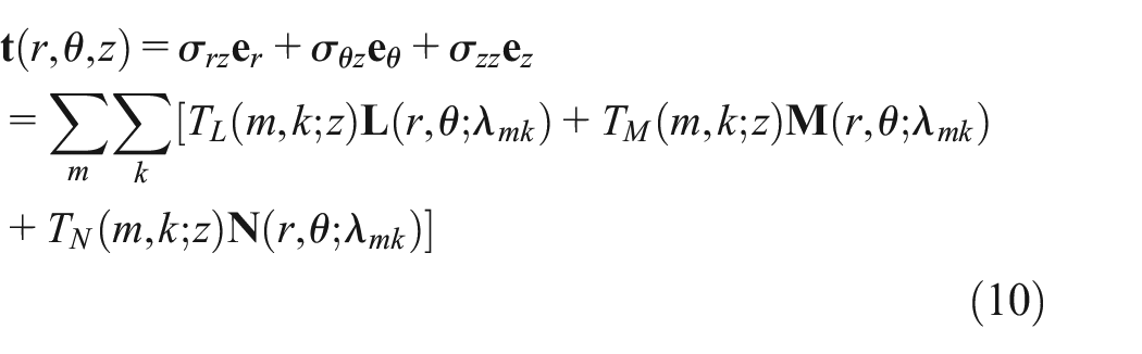
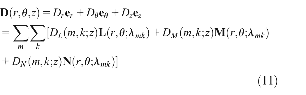
whilst the electric potential φ function can be expanded as
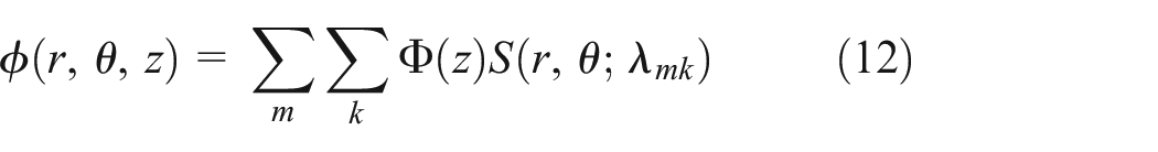
where UL, UM, UN, TL, TM, TN, DL, DM, DN, and
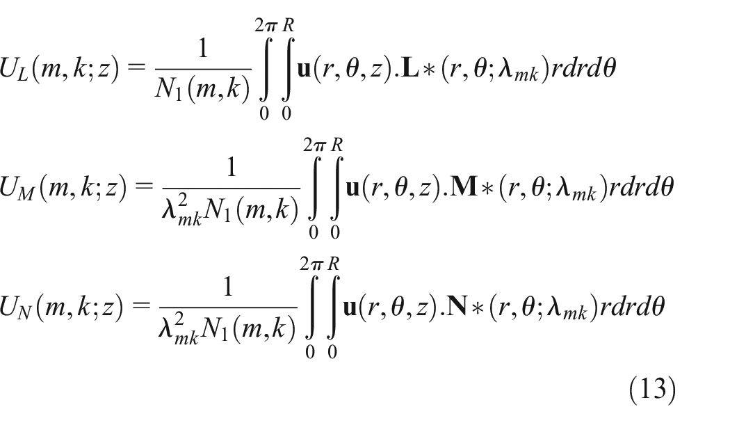
and the expansion coefficient of the electric potential in equation (12) can be expressed as
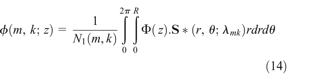
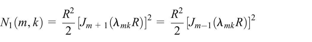
where * means the complex conjugate, and
It is noteworthy, for the axis-symmetric deformation, that is, m = 0, only LM-type vector functions will be involved. However, under a horizontal load, we have m = ±1 and thus both LM
From the constitutive relations, we find the following relations among the expansion coefficients of the traction, electric displacement, elastic displacement, and electric potential
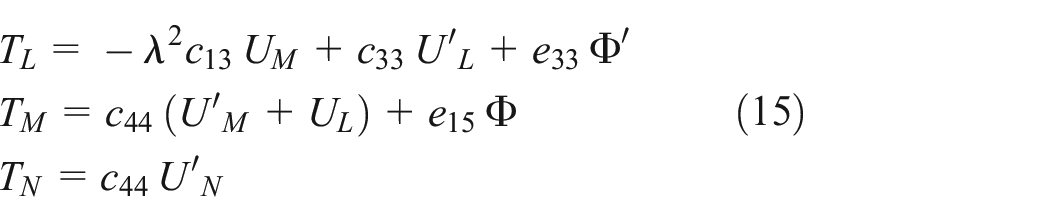
and

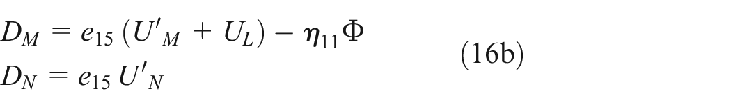
where prime denotes derivative with respect to the coordinate variable z.
Equations (15) and (16a) contains eight expansion coefficients and needs to be combined with the following three relations (from equations (1) to (3)) to solve them
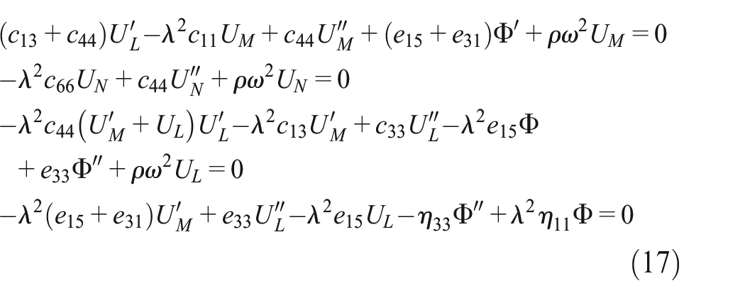
Now equations (15), (16a), and (17) contain a total of eight equations for the eight expansion coefficients that is, UL, UM, UN,
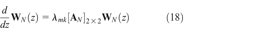
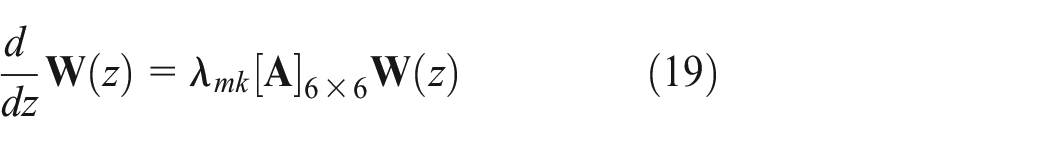
For the N-type, we have the following standard linear system of ordinary differential equations
For the LM-type, we have
where coefficient matrices
It is noted here that the LM-type system corresponds to the P-, SV-, and Rayleigh-waves whilst the N-type corresponds to the SH- and Love-waves. If the applied load is axis-symmetric, the N-type solution is zero.
3.2. General solution in each layer
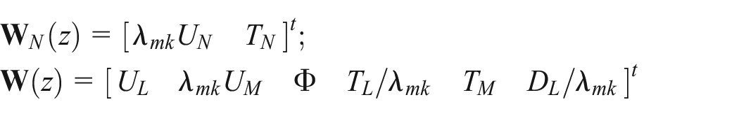
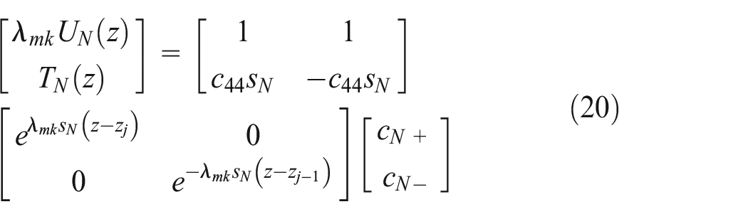
The solutions of equations (18) and (19) can be simply expressed in terms of their eigenvalues and eigenvectors. The general solutions in any layer, say in Layer j bounded by zj−1 and zj, that is,
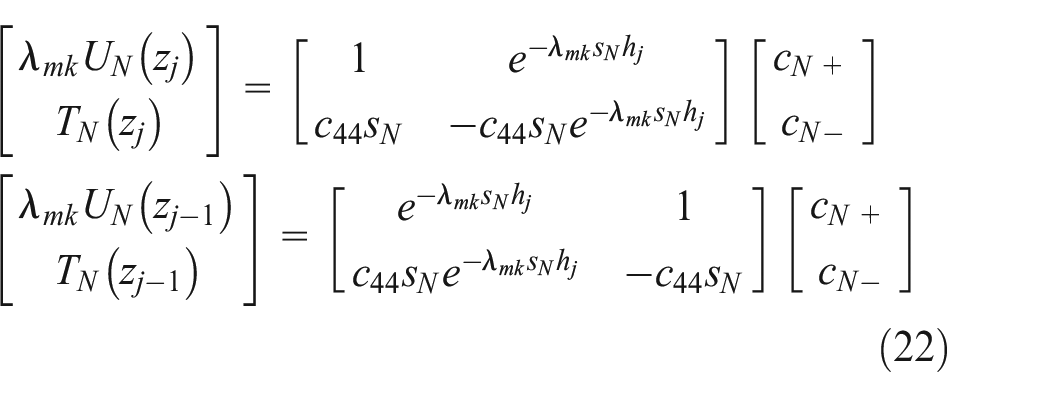
For N-type,
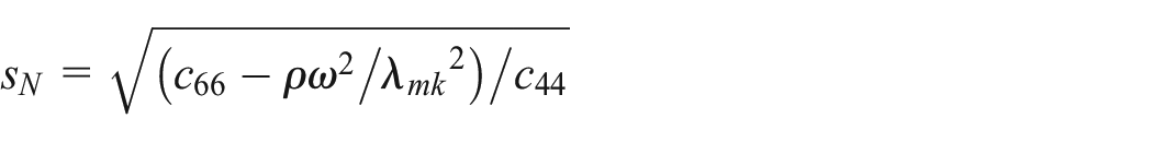
where
For LM-type,
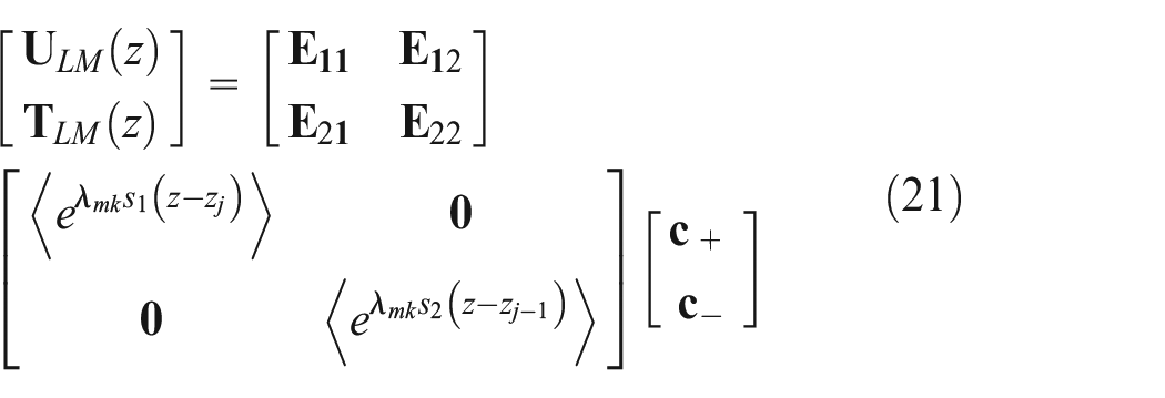
where
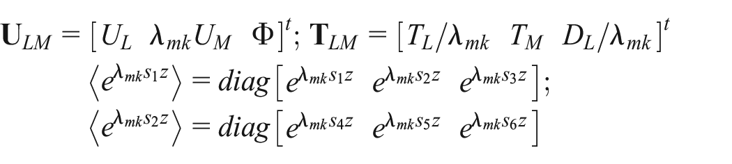
and
Notice that for the N-type in equation (20), sN has a positive real part. For the LM type in equation (21), the first three eigenvalues all have positive real parts and the other three have negative real parts. Thus, we have Re(s1)≥…≥Re(s4).
3.3. Solution in the layered half–space
3.3.1. DVP matrix and recursive relations
In order to obtain the time-harmonic solution in a multi-layered TI-PE half-space, the DVP method is adopted. This new DVP method is unconditionally stable, flexible, and powerful for problems having high frequency, material anisotropy, imperfect interface, and many more. First, equations (20) and (21) can be written on the interfaces of Layer j
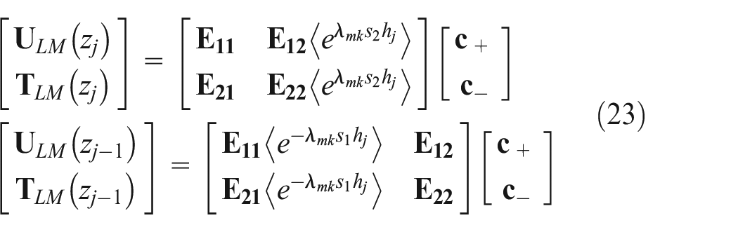
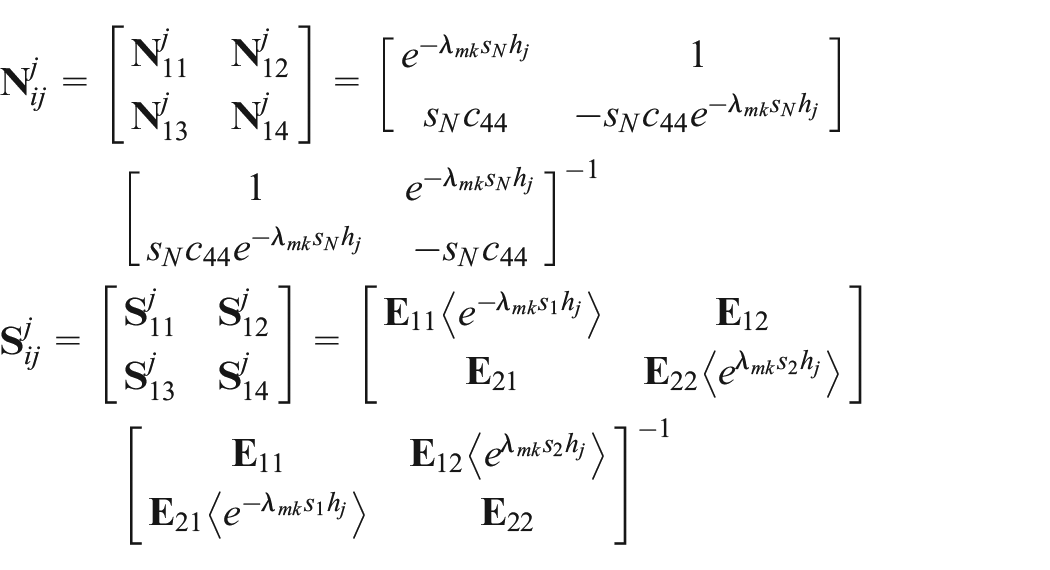
where hj = zj−zj−1. Then, by eliminating the constants
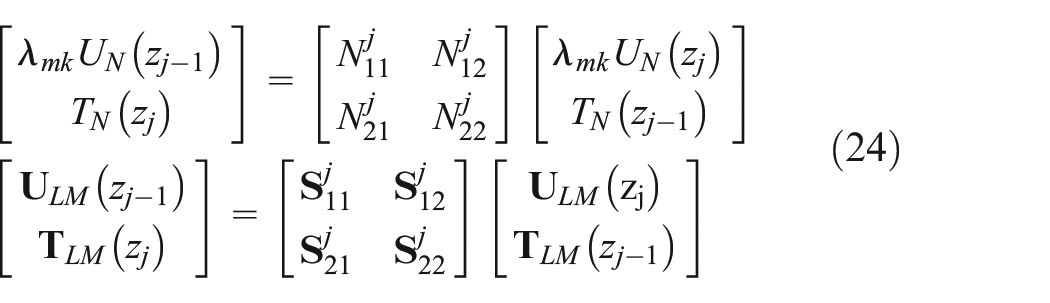
where the submatrices are given by
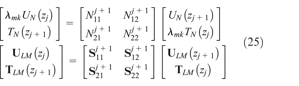
Similarly, the expansion coefficients for Layer j + 1 are
Assuming that the interface between the two layers is well bonded (i.e. the elastic displacements, tractions, electric displacement in z-direction, and electric potential are continuous), we then find the following important recursive relation from Layer j to Layer j + 1 as
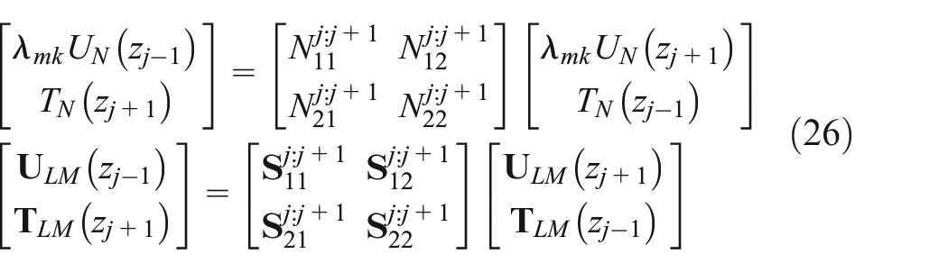
where the superscripts j:j+1 denote the propagated submatrix from Layer j to Layer j+1 given by
The new recursive relation (i.e. equation (26)) can be propagated in the layered structure, as long as the interfaces are perfect, or well-bonded. By applying it repeatedly from the bottom layer to the top or vice versa, the unknown expansion coefficients at the top and bottom interfaces can be connected. By utilizing the boundary conditions given, the involved known coefficients can be solved. After that, equation (26) can be utilized to find the expansion coefficients at any depth.
4. Boundary conditions
4.1. Boundary conditions on the surface in terms of expansion coefficients
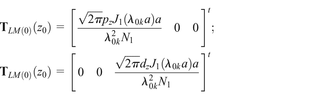
For the given time-harmonic load within the circle of radius a on the surface (Figure 1), the following expansion coefficients in term of FBS system are found as (Pan et al., 2021)
The following three separate cases are considered in this paper.
Case 1: Under uniform vertical load pz, we have
Case 2: Under uniform vertical electric displacement dz, we have
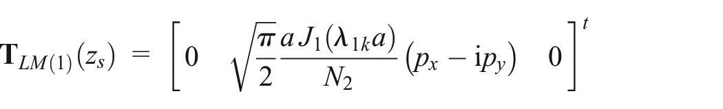
Case 3: Under uniform horizontal load (px, py) in both x- and y-directions, we have
4.2. Expansion coefficients of displacements and electric potential on the surface
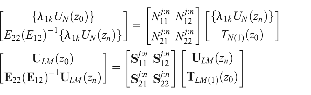
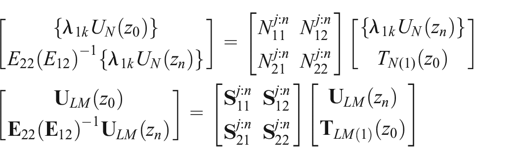
With the given general surface traction expansion coefficients and the derived recursive relation, we can propagate the expansion coefficients from the surface z0 to the last layer interface zn to obtain the following relations
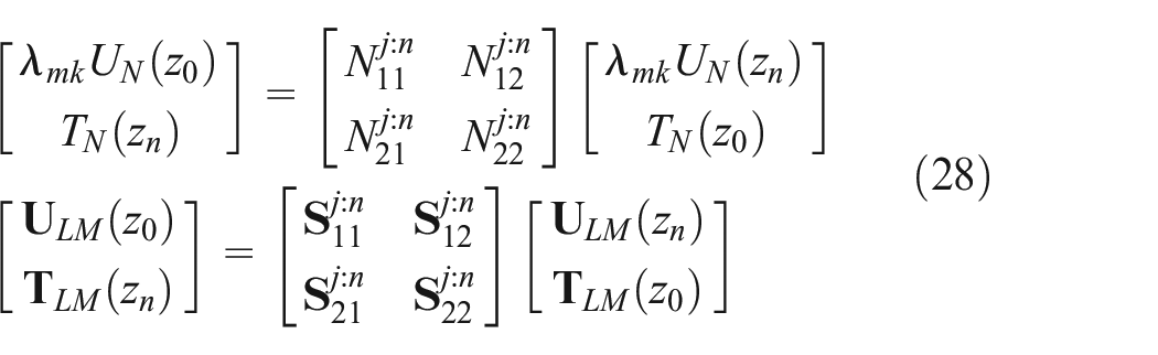
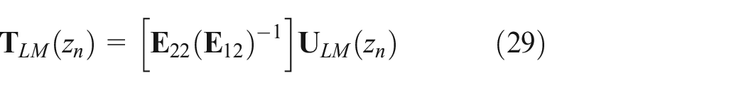
On the last interface z = zn, the unknown coefficients in equation (28) are related as, for the LM-type (similar expression for the N-type)
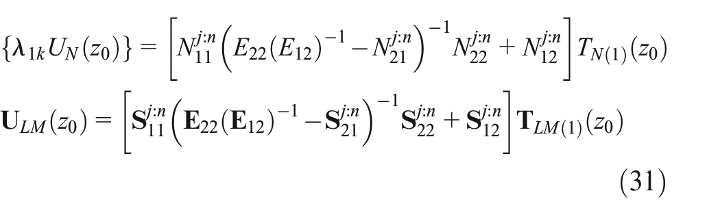
By substituting equation (29) into equation (28), we have the following relations for different loading cases.
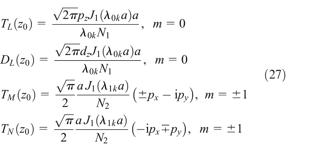
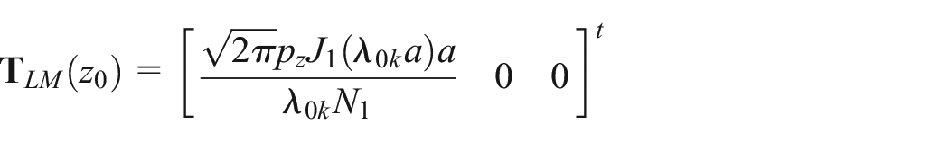
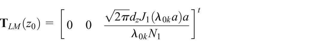
(1) Under the vertical symmetric load (i.e. for m = 0) we have only the LM-type solution, which is
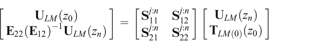
for which the solution on the surface is given by
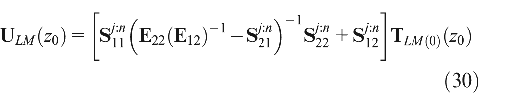
where
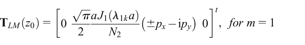
(2) Under the horizontal load (i.e. for m = ±1), we have both N-type and LM-type solutions, which are given below
For m = 1, we have
with the solution on the surface being
where
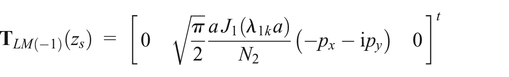
Similarly, for m = −1, we have
with the solution on the surface being
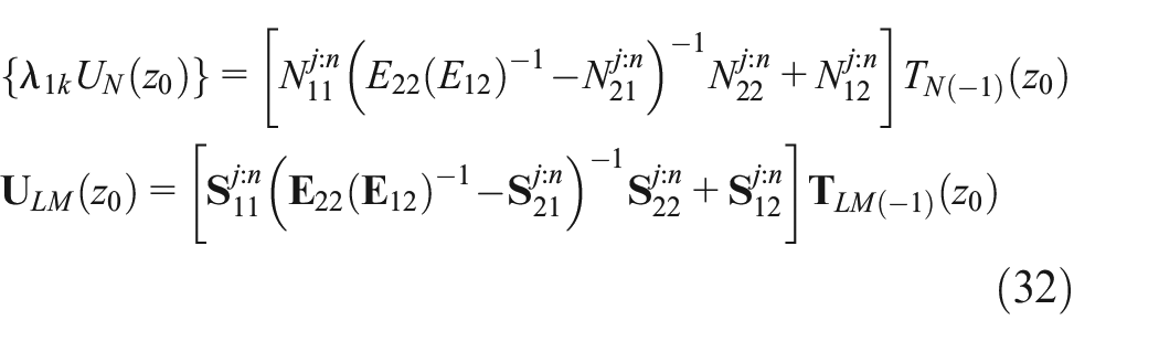
where
Once the expansion coefficients on the surface and last interface are solved, we can just simply carry out the summation (i.e. equations (9)–(12)) to find the frequency-domain solution at any physical point on the surface. After that, we only need to replace z0 by z in equation (28) in order to find the solutions at different z-levels. We point out again that since these coefficients are discrete numbers, they are the exact Love numbers which can be pre-calculated and saved for later use in the corresponding Green’s function calculation (i.e. Zhou et al., 2023).
5. Numerical studies
Before presenting numerical examples, we first remark that our newly derived solution has been verified with existing solutions in the literature. These results are consistent with those reported in Han et al. (2006), Pan et al. (2021), and Qi et al. (2023). Appendix B contains a few graphs which demonstrate the accuracy of the present new method as compared with those in Pan et al. (2021) and Qi et al. (2023). Then, the present solution is applied to the time-harmonic loads (mechanical and electrical), which are uniformly applied over a circular patch of radius a on the surface of a layered TI-PE half-space structure for an electrically open circuit case. An FBS MATLAB program is written, which is very powerful and can handle easily multiple loads along with material anisotropy. To avoid the singularities, the elastic properties are perturbed away from their real values by multiplying a small material damping factor β. Namely, ckj, ekj, and ε kj are replaced by ckj (1 + 2iβ), ekj (1 + 2iβ), and ε kj (1 + 2iβ) in the numerical calculation. Also in the paper, all numerical results are presented in the dimensionless form, defined as
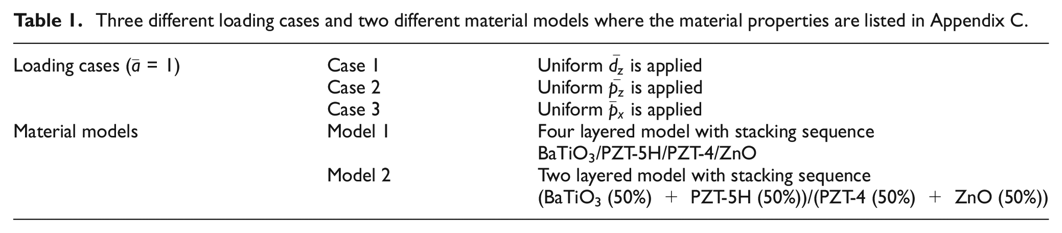
Here φmax = Emax/a. The value of Cmax and Emax for Model 1 is 210.9 × 10⁹ N/m2 and 17 C/m2, respectively. For Model 2, they are Cmax = 174.1 × 10⁹ N/m2 and Emax = 20.95 C/m2.
To study how the static and dynamic loads affect the piezoelectric response, two models are constructed, along with the three loading cases, that is, vertical electrical load
Three different loading cases and two different material models where the material properties are listed in Appendix C.
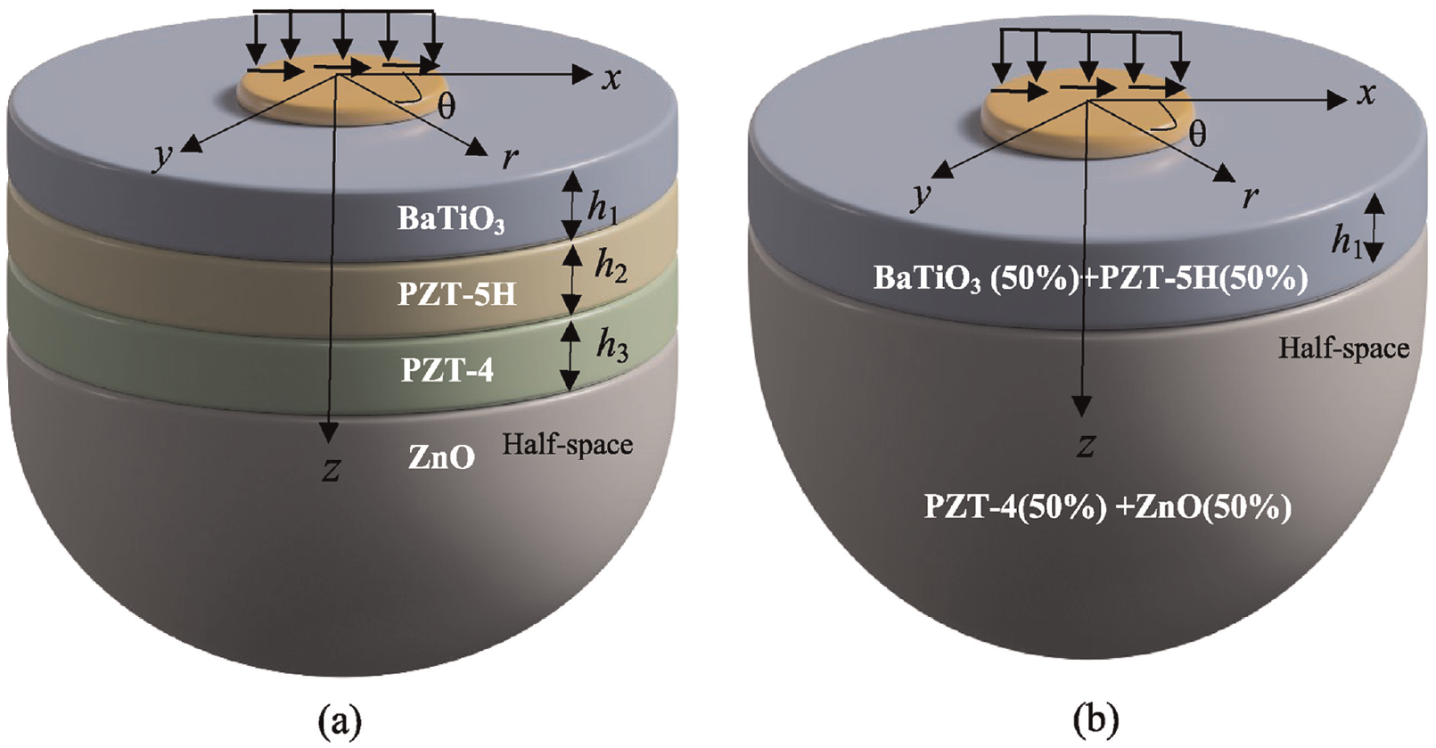
Geometry of the four-layered structure (a) and two-layered structure (b).
5.1. Four-layered model
The time-harmonic response subjected to the circular vertical electrical load
Variation of dimensionless displacement
Variation of the dimensionless displacement
Variation of the dimensionless displacement
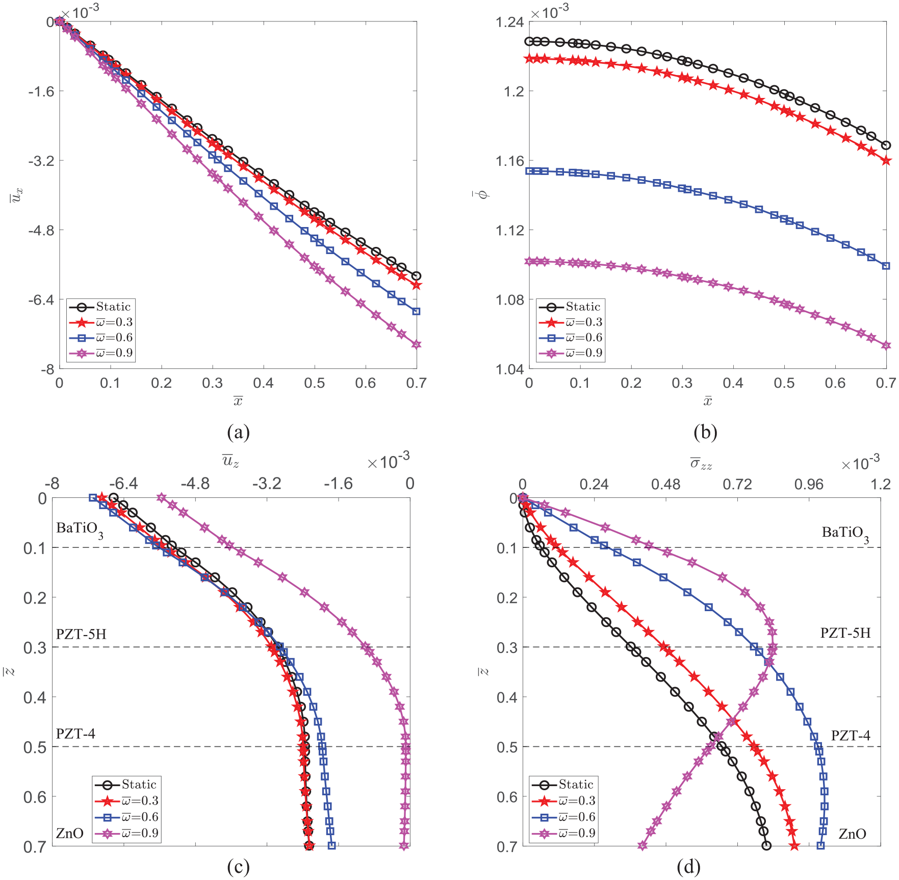
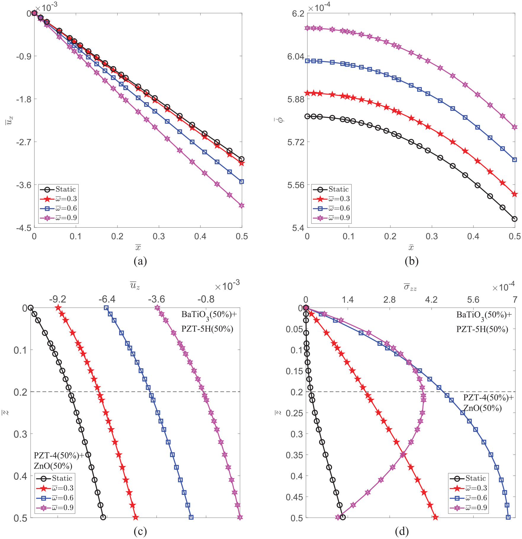
5.1.1. Under vertical electric displacement
Figure 3(a) and (b) depicts the spatial distribution of the dimensionless mechanical displacement
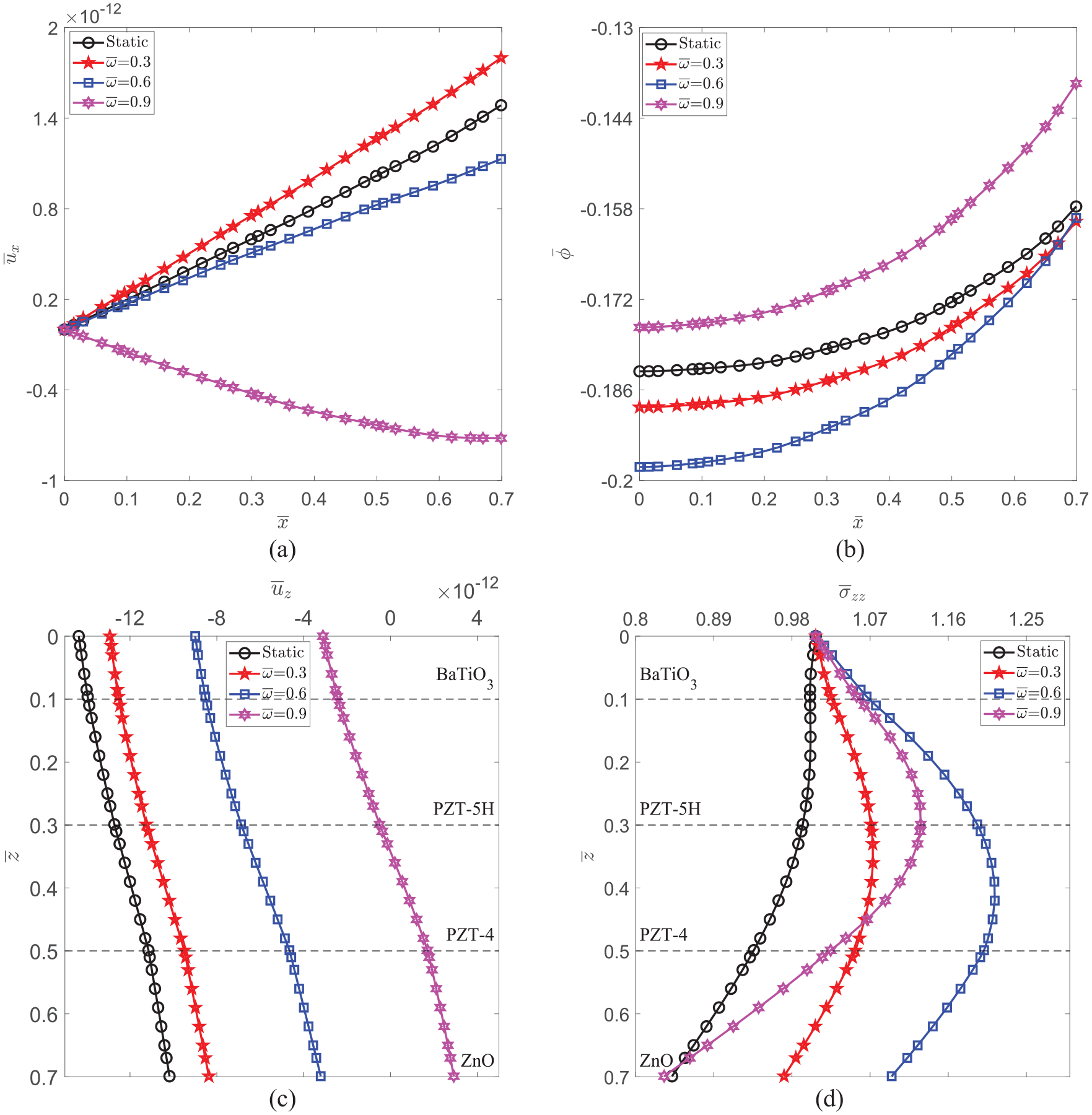
5.1.2. Under vertical mechanical load
Figure 4(a) shows that the magnitude of the dimensionless displacement
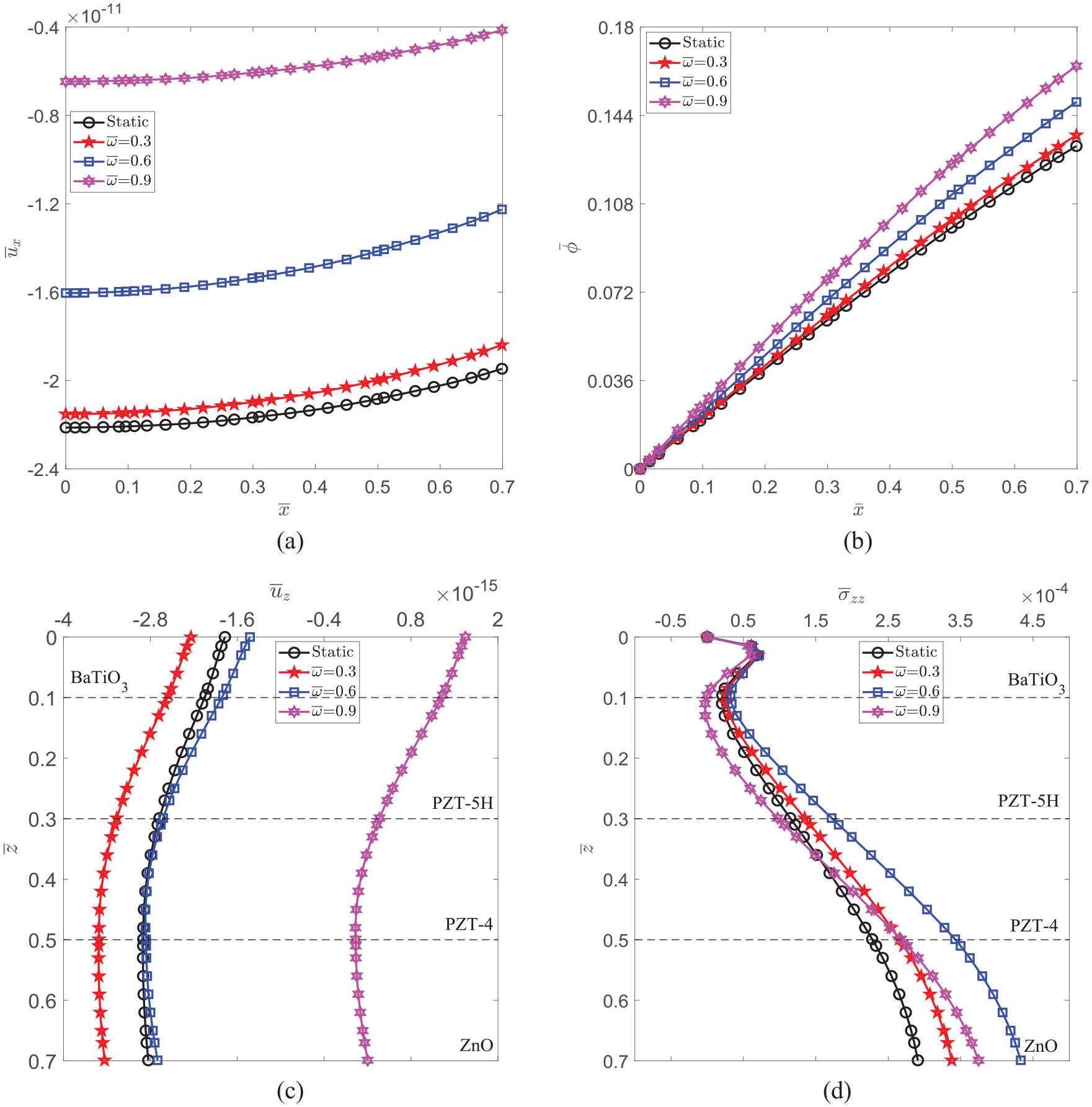
5.1.3. Under horizontal mechanical load
Figure 5(a) and (b) show the variation of the dimensionless displacement
Figure 5(c) shows the variation of
5.2. Two-layered model
We now study the time-harmonic response in the “equivalent two-layered half-space,” that is, Model 2. Notice that the material properties are from those in the four-layered half-space by taking the two-layer average. The applied loads are the same, namely, a uniform vertical electric load
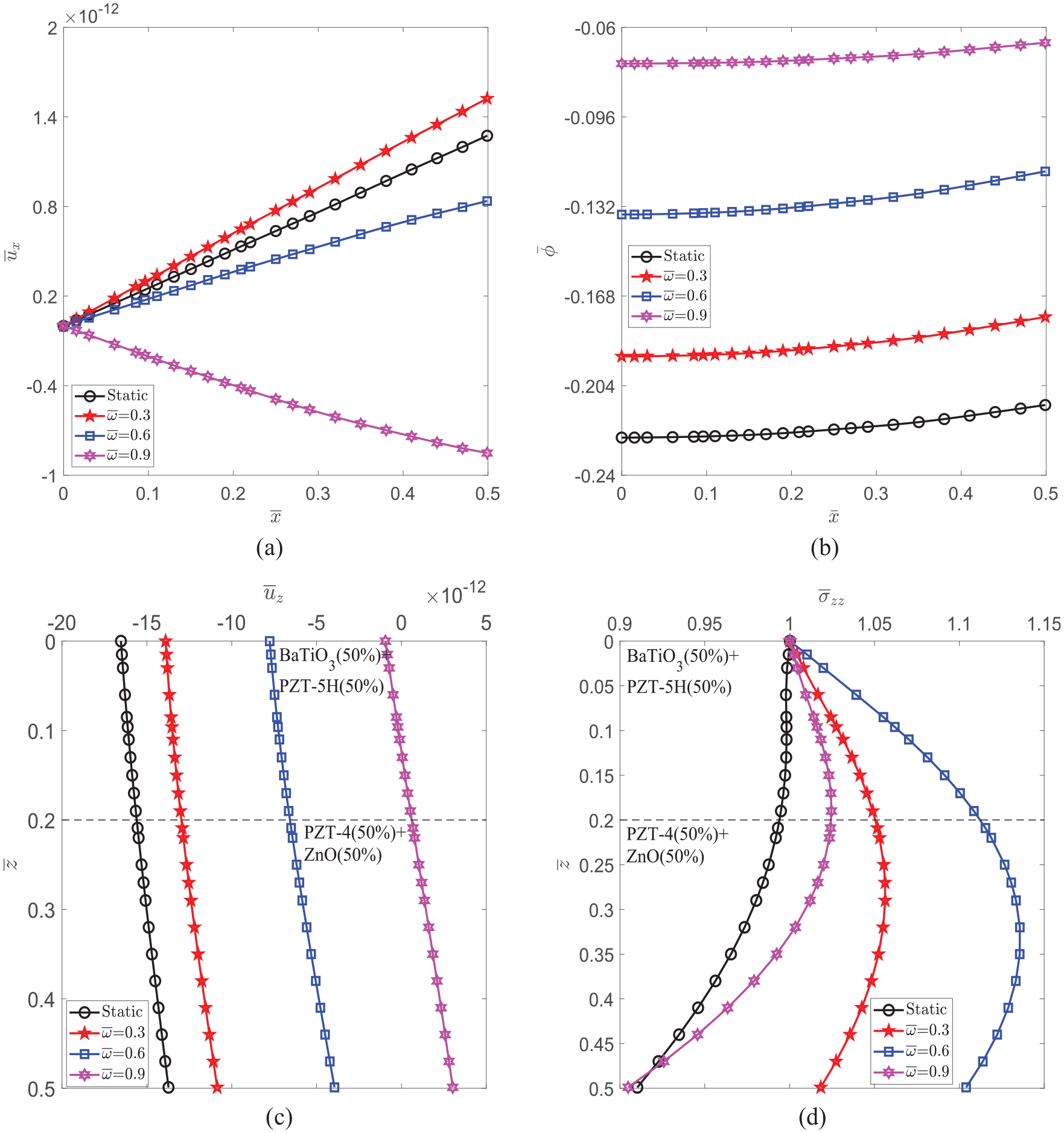
5.2.1. Under vertical electric displacement
Figure 6(a) to (d) depict the variation of the dimensionless elastic displacement
Variation of the dimensionless displacement
Compared to those in the four-layered half-space in Figure 3(a) to (d), we observe that, while some patterns are similar, significant differences exist as clearly shown in Figure 6(b) and (c). Notably, Figure 6(b) reveals that, for fixed
5.2.2. Under vertical mechanical load
Figure 7(a) to (d) show the distribution of dimensionless mechanical displacement
Variation of the dimensionless displacement
Figure 7(b) shows a significant impact of frequency on the magnitude of the electric potential. Namely, an increase in frequency could cause the electric potential
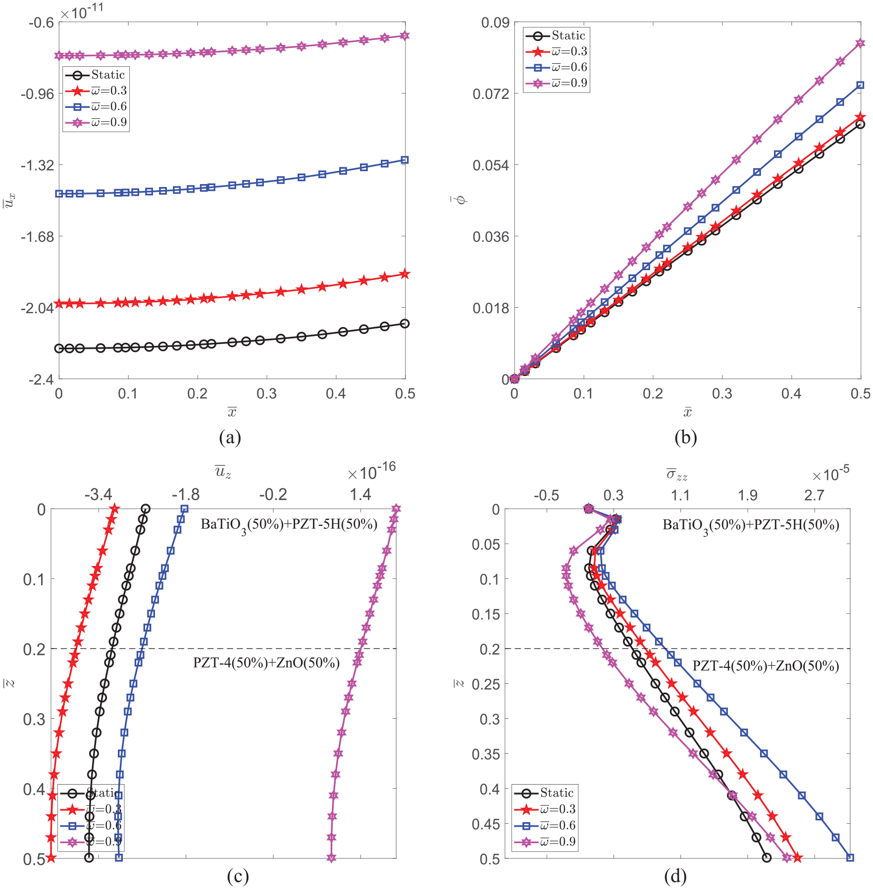
5.2.3. Under horizontal mechanical load
Figure 8(a) to (d) depict the distribution of dimensionless mechanical displacement
Variation of the dimensionless displacement
6. Conclusion
The time-harmonic response of a transversely isotropic piezoelectric layered half-space induced by surface loading is solved. Two different material models, four-layered and two-layered, are considered (each constituted by a different class of PE materials) to understand the complexity of the responses in the coupled structure. The novel and computationally powerful Fourier-Bessel series (FBS) system of vector functions and the dual-variable and position (DVP) method are employed to solve the boundary-value problem accurately and efficiently. Via numerical examples, the following conclusions can be drawn:
The effect of input frequency on the horizontal displacement
Under a vertical mechanical load, the effect of frequency on the displacement
Under a horizontal mechanical load, the response behavior is similar to those under a vertical mechanical load. However, their variations along
Footnotes
Appendices
Declaration of conflicting interests
The author(s) declared no potential conflicts of interest with respect to the research, authorship, and/or publication of this article.
Funding
The author(s) disclosed receipt of the following financial support for the research, authorship, and/or publication of this article: This study was financially supported by the National Science and Technology Council of Taiwan (Grant No. NSTC 111-2811-E- 516 A49-534).