
Abstract
This article presents a tunable multi-stable piezoelectric energy harvester. The apparatus consists of a stationary magnet and a cantilever beam whose free end is attached by an assembly of two cylindrical magnets that can be moved along the beam and a small cylindrical magnet that is fixed at the beam tip. By varying two parameters, the system can assume three stability states: tri-stable, bi-stable, and mono-stable, respectively. The developed apparatus is used to validate two models for the magnetic restoring force: the equivalent magnetic point dipole approach and the equivalent magnetic 2-point dipole approach. The study focuses on comparing the accuracy of the two models for a wide range of the tuning parameters. The restoring forces of the apparatus are determined dynamically and compared with their analytical counterparts based on each of the models. To improve the model accuracy, a model optimization is carried out by using the multi-population genetic algorithm. With the optimum models, the parametric sensitivity of each of the models is investigated. The stability state region is generated by using the optimum second model.
Keywords
1. Introduction
In this century, wireless sensor networks have been playing an important role in the Internet of Things (IoT). Normally, the wireless sensors are powered by batteries which are not eco-friendly. It has been much desirable to use vibration energy harvesters to solve costly battery replacement problem and make wireless sensor networks autonomous (Tian et al., 2018). Ambient vibration can be converted to electricity by four methods: piezoelectric (Derayatifar et al., 2021; Lu et al., 2018), electromagnetic (Halim et al., 2015; Pan et al., 2019; Williams and Yates, 1996; Zaghari et al., 2019), electrostatic (Choi et al., 2011; Koga et al., 2017; Zhang et al., 2018), and triboelectric (Tao et al., 2020; Wang et al., 2018b). The main advantages of the piezoelectric vibration energy harvesters (PVEHs) are their large power densities and ease of operation.
A traditional PVEH is a single-degree-of-freedom linear oscillator that performs efficiently only at resonance (Roundy and Wright, 2004; Roundy et al., 2003; Yu and He, 2013). To broaden the response frequency bandwidth, various nonlinear energy harvesters have been proposed (Ramlan et al., 2010; Twiefel and Westermann, 2013; Yang et al., 2018, 2019). According to the system stability, the nonlinear PVEHs can be classified as mono-stable and multi-stable, such as bi-stable or tri-stable. The nonlinearity can be realized by introducing the nonlinear restoring forces to the piezoelectric beam. Applying magnetic forces to the beam is one of the convenient ways to achieve that. Stanton et al. (2009) reported a PVEH that consists of a piezoelectric cantilever beam with a tip magnet subjected to an external magnetic field generated by a pair of fixed magnets. Such a mono-stable energy harvester can exhibit softening or hardening behaviors when the magnetic interaction is adjusted. By applying different external magnet tuning strategies, two kinds of bi-stable energy harvester (BEH) can be achieved: attractive magnetic force type (Fu and Yeatman, 2019; Rezaei et al., 2021) or repulsive magnetic force type (Bae and Kim, 2021; Wang et al., 2018a; Xie et al., 2019). Zhao and Erturk (2013) found that for a certain range of excitation intensity, the BEH can largely enhance the power output performance due to its snap-through characteristic. Further, in order to reduce the potential barrier of BEHs, tri-stable energy harvesters (TEH) have been proposed by introducing a middle potential well between BEH’s two potential wells. Based on the configuration of the BEH proposed by Erturk et al. (2009), TEHs were achieved by tuning the angular orientations (Cao et al., 2015; Zhou et al., 2013) or the spatial positions (Haitao et al., 2016; Wang et al., 2019) of the two fixed magnets. However, the disadvantage of the aforementioned tunable multi-stable PVEHs is that they need more than one fixed magnet to achieve the tri-stable state. Thus, installing multiple fixed magnets would take more space, which is undesirable in realization through a micro-electromechanical system (MEMS). And also, an asynchronous operation of tuning the angle or position of the fixed magnets will lead to the asymmetric potential wells for the TEH.
In the dynamic modeling of a tunable multi-stable PVEH, an accurate magnetic force model is crucial. Generally, the magnetic force between two magnets is complicated, especially when the separation distance between them is relatively small. There are several commonly used models for this purpose. The most widely used one is the so-called equivalent magnetic point dipole approach (Fang et al., 2019; Stanton et al., 2010; Tang and Yang, 2012) which treats each magnet as a point dipole at its center. However, this approach has a limitation as it can offer a reliable prediction only when the distance between the magnets is much greater than their dimensions. In light of this limitation, a magnetic force modeling method based on the equivalent magnetizing current theory was proposed (Leng et al., 2017; Tan et al., 2015). The study indicates that the magnetizing current model offers better accuracy than the equivalent magnetic point dipole model. Accordingly, Wang et al. (2020) proposed an equivalent magnetic 2-point dipole approach, which only counts the magnetizing current on the permanent magnet’s left and right polarized surfaces and uses two total surface charges to represent a magnet. It has been proved that the accuracy of the equivalent magnetic 2-point dipole model was significantly improved by using the proposed method (Ju et al., 2021; Rezaei et al., 2021; Wang et al., 2020; Zhang et al., 2021). Currently, such approach is mainly used in the modeling of the magnetic force between thin cubic permanent magnets, the accuracy of the magnetic force model of the thick cylinder magnets based on such approach still needs to be examined.
In this study, a new tunable multi-stable piezoelectric energy harvester is proposed. Different from the existing design which employs multiple fixed magnets to achieve a tri-stable state, the proposed apparatus consists of a stationary magnet and a cantilever beam whose free end is attached by an assembly of two cylindrical magnets that can be moved along the beam and a small cylindrical magnet that is fixed at the beam tip. By varying the gap between the stationary magnet and the tip magnet, and the distance between the magnet assembly and the tip magnet, the system can assume three stability states: tri-stable, bi-stable, and mono-stable, respectively. Modeling the magnetic restoring forces for a tunable multi-stable energy harvester poses a challenge as a reliable model should give an accurate prediction over a wide range of the tuning parameters. For this purpose, the developed apparatus is used to dynamically validate two commonly used models: the equivalent magnetic point dipole approach and the equivalent magnetic 2-point dipole approach proposed by Wang et al. (2020). The study shows that although the second model offers more accurate results than the first model, it still fails to predict the restoring forces in some cases. A numerical optimization is carried out to improve the accuracy of both models. The study shows that by using the optimum parameters, both models can achieve a comparable accuracy.
The rest of the paper is organized as follows. Section 2 presents the proposed apparatus. Section 3 derives the magnetic restoring force models based on the equivalent magnetic point dipole approach and the equivalent magnetic 2-point dipole approach, respectively. Section 4 validates the two models dynamically. Section 5 conducts a model optimization. Section 6 uses the optimum model for the parametric sensitivity study and the stability region determination. Finally, Section 7 draws the main conclusions of the study.
2. Apparatus
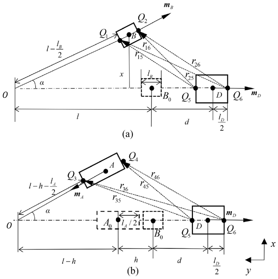
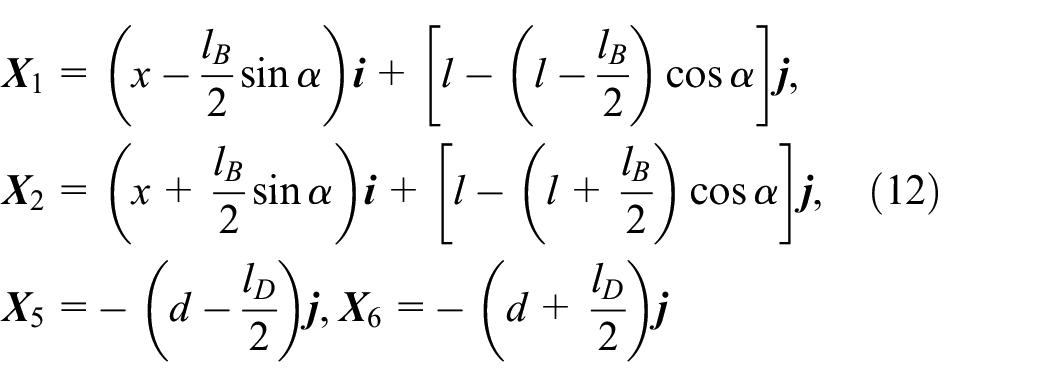
Figure 1 shows a CAD drawing of the developed apparatus. A cantilever beam is constructed by connecting a piezoelectric transducer (S128-J1FR-1808YB, Midé) to a thin stainless-steel plate. One end of the cantilever beam is clamped to a stand that is fastened to a base, while its other end is fixed with a small cylindrical magnet B and attached with a holder for an assembly of two identical cylindrical magnets A and C. The holder for magnets A and C can slide along the beam. A large cylindrical magnet D is fixed in a stand that can slide along the base. When the cantilever beam is at its equilibrium position or undeflected, the four magnets situate on the same vertical plane and magnets B and D are collinear. By sliding the stand for magnet D, the distance between magnet B and magnet D can be adjusted. By sliding the holder along the beam, the distance between magnet B and magnets A, C can be varied. Figure 2 illustrates the spatial positions and polarities of the four magnets where
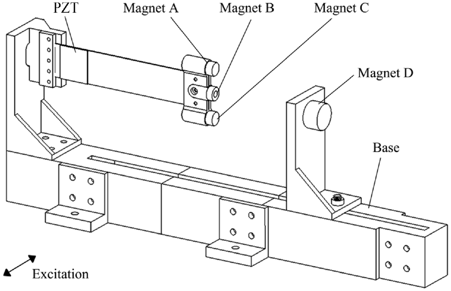
Schematic of the apparatus.
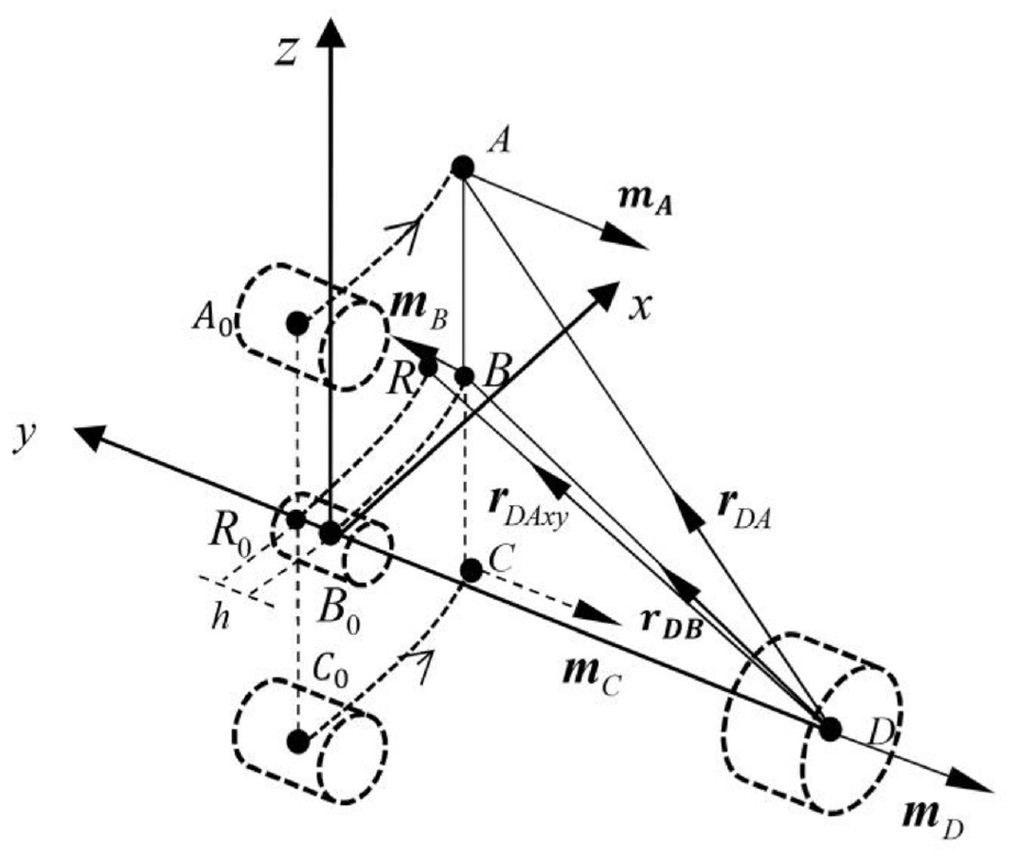
Spatial positions of the magnets.
Figures 3 and 4 show the front view and top view of Figure 2, respectively, where d is the distance between magnet D and magnet B when the beam is undeformed, and
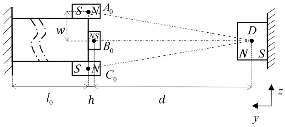
Front view of the apparatus.
Top view of the apparatus.
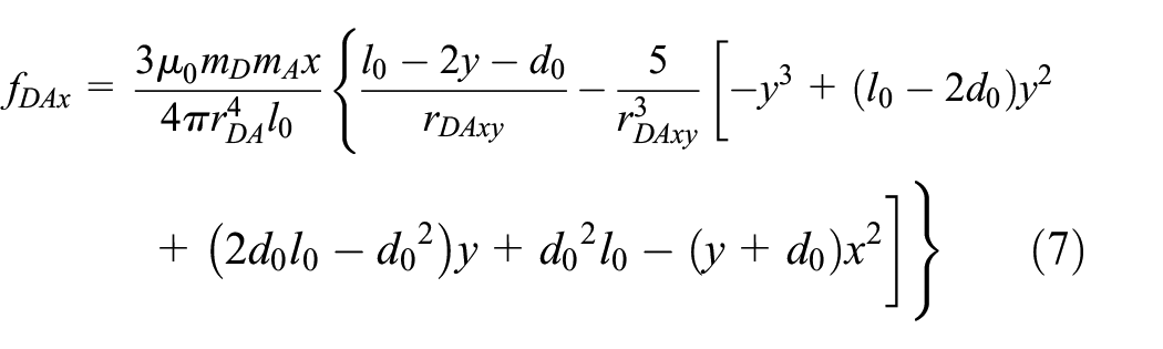
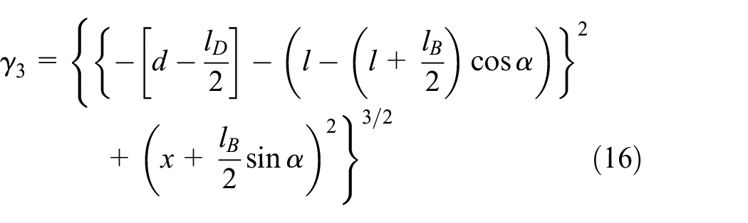
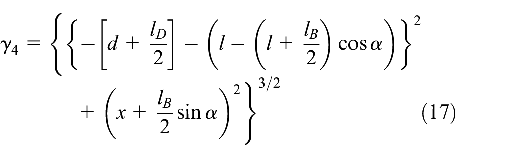
3. The restoring force of the system
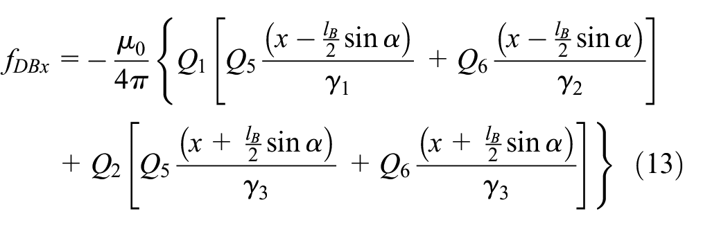
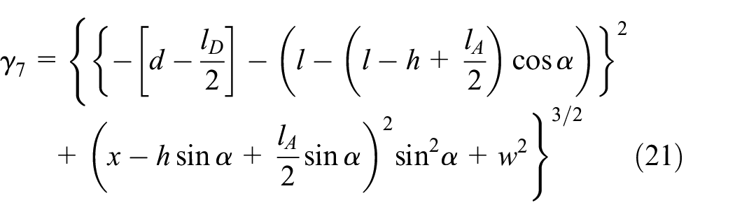
The total restoring force

where
3.1. Equivalent magnetic point dipole model
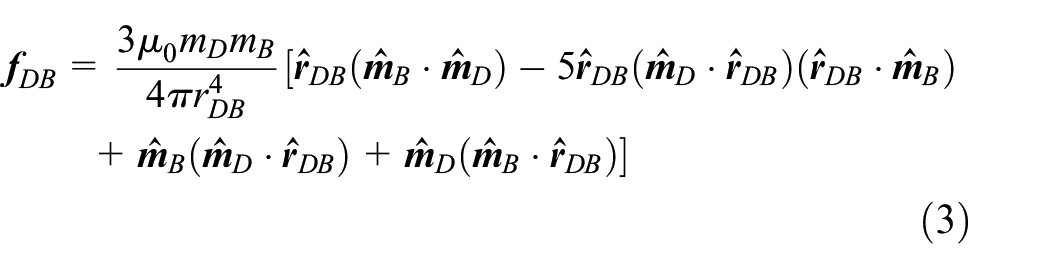
Commonly, a pair of magnets is regarded as equivalent magnetic point dipoles by assuming that the magnet sizes are much smaller than their separation distance (Yung et al., 1998). Firstly, the magnetic force between magnet B and magnet D is considered. According to this approach, the force exerted by magnet B on magnet D is given by:

where ∇ denotes the vector gradient operator and
where
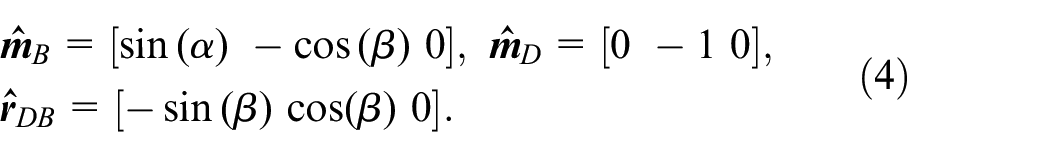
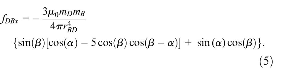
Substituting the above unit vectors in equation (3) and the magnetic force in the x-direction can be obtained in the following form:
Since the slope of the beam’s tip is relatively small, it is assumed that
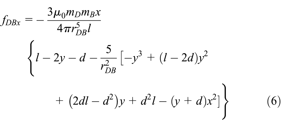
where
where

where
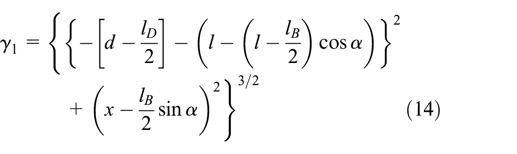
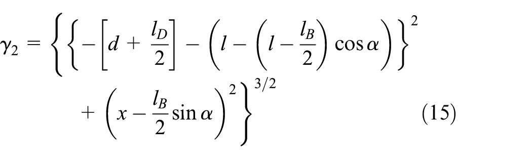
3.2. Equivalent magnetic 2-point dipole model
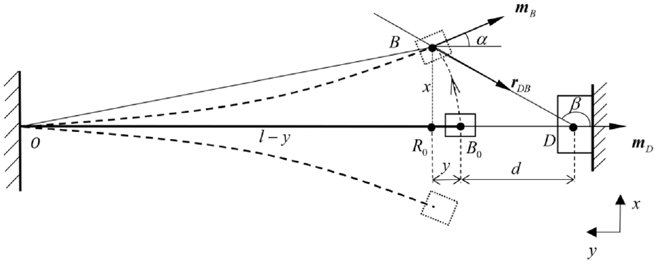
As Leng et al. (2017) mentioned, the equivalent magnetic point dipole approach’s accuracy deteriorates when the separation space between the magnets becomes small. In light of such limitation, an improved approach was proposed by Wang et al. (2020). In this study, such an improved approach is named as equivalent magnetic 2-point dipole model as the approach treats a magnet as a 2-point dipole. In what follows, the magnetic restoring force of the system is developed using this improved method. Figure 5(a) and (b) show the top view of the apparatus when the beam is deformed.
Top view of positions of magnets of the apparatus: (a) magnet B and D and (b) magnet A and D.
As shown in Figure 5(a) and (b), the origin of the coordinate system locates at
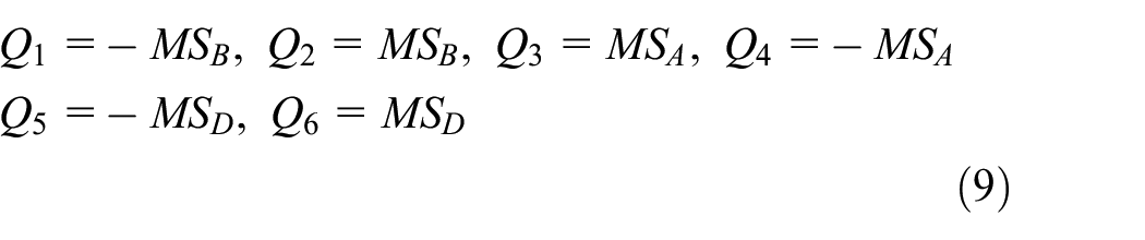
where
Similar to the previous section, the magnetic force between magnet B and magnet D is considered first. Based on the Boit-Savart law, the magnetic force exerted by magnet B on magnet D is the combination of the magnetic force exerted from

where
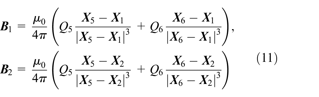
were
where
where
By following the same process, the magnetic force between magnet A and D in the x-direction can also be obtained as:
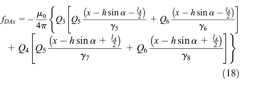
where

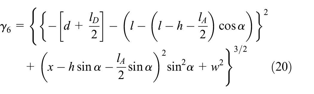

where w is the distance between magnets A and B in the z-direction, which can be observed in Figure 3. By substituting equations (13) and (18) into equation (1), the total restoring force can be obtained.
4. Experimental validation
With the models established, a natural question arises regarding their accuracy and reliability. To this end, an experimental model validation is conducted. For simplicity, hereinafter, the equivalent magnetic point dipole model and 2-point dipole model are referred to as first model and second model, respectively. The restoring force surface method (Worden, 1990) is employed to determine the total restoring forces dynamically. Figure 6(a) and (b) show the experimental setup and the detail of the magnets’ positions, respectively. Figure 6(c) shows a schematic of the equivalent lumped parameter model that represents the experimental setup, where

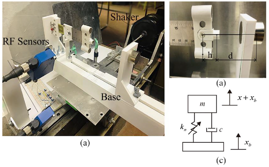
(a) Photo of the experimental setup, (b) detail of the beam, and (c) schematic of the equivalent lumped parameter model for the experimental setup.
where

where
As shown in Figure 6(a), the apparatus is mounted on a slipping table that is driven by a shaker (2809, Brüel & Kjær) through a stinger. The shaker is driven by an amplifier (2718, Brüel & Kjær). Two laser reflex sensors (RF) (CP24MHT80, Wenglor) are used to measure the transverse displacement of the beam’s tip and the base’s displacement, respectively. A computer equipped with the dSPACE dS1104 data acquisition board is used to collect sensor data and send voltage signal to the power amplifier to drive the shaker. The control program is developed by using the MATLAB Simulink which is interfaced with dSPACE Controldesk Desktop software. The velocity and acceleration are obtained by numerical differentiation of the measured displacement signals.
To apply the restoring force method properly, the responses should sufficiently cover the phase plane. The exciting signal should be persistently strong so that both intrawell and interwell responses are established. For this purpose, a harmonic signal with a slowly modulated amplitude is employed

where
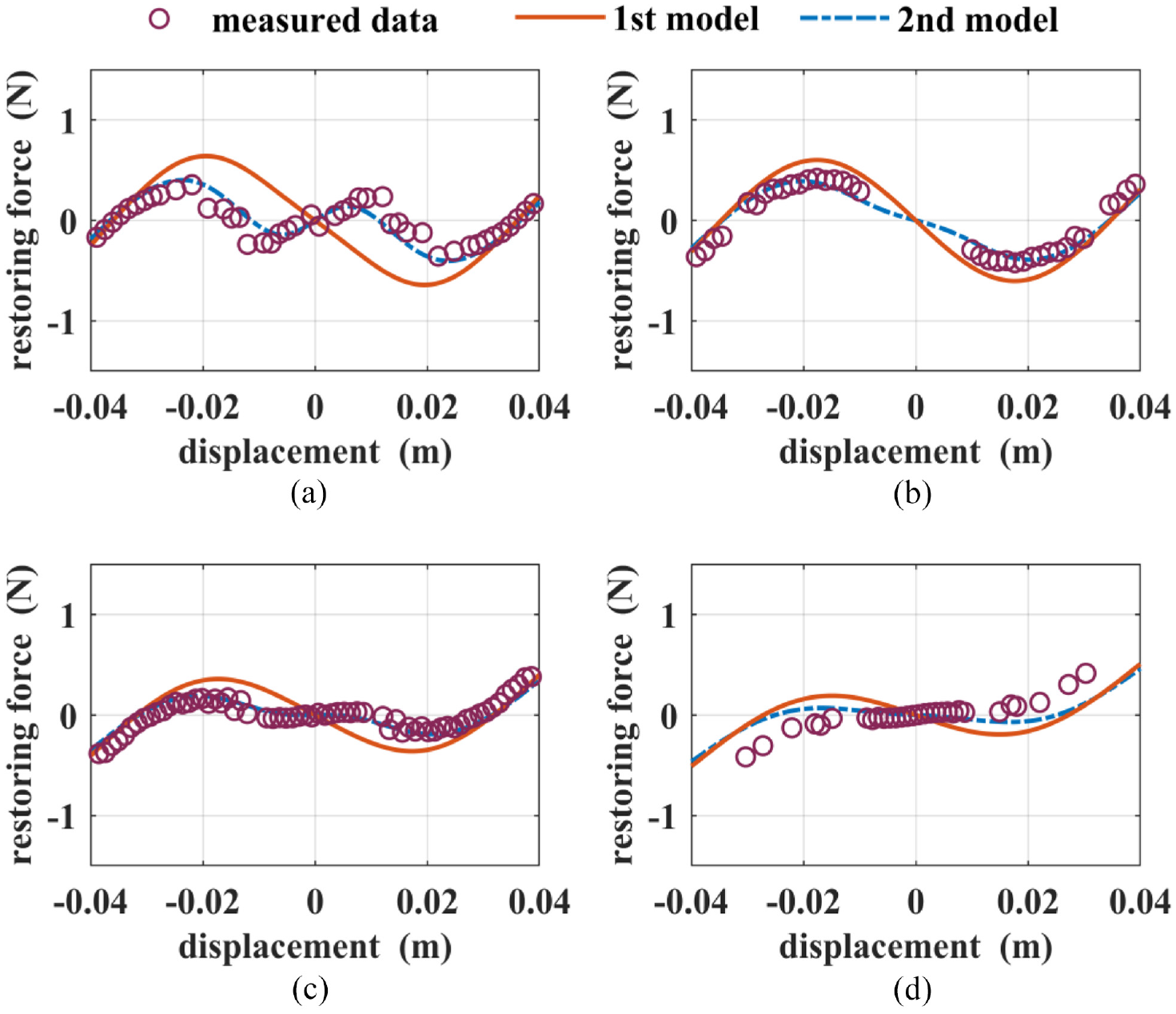
The total restoring forces of: (a) Case (1), (b) Case (2), (c) Case (3), and (d) Case (4).
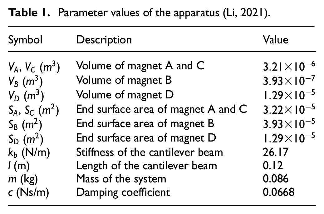
Parameter values of the apparatus (Li, 2021).
5. Model optimization
As shown in the previous section, although the second model gives a better prediction for the restoring force than the first model in Cases (1), (2), and (3), it fails to do so in Case (4). It is natural to ask a question of whether both models can be improved by optimization. For this purpose, an optimization based on the multi-population genetic algorithm (MPGA) (Kim and Khosla, 1992) is carried out to identify the magnitudes of the magnetic vectors for the first model, and the amounts of the total charges for the second model. Different from the standard genetic algorithm, which only has a single population group, the MPGA initializes the whole population as multiple population groups to operate the selection, crossover, and mutation independently. Figure 8 shows the flowchart of the MPGA. Note that the flowchart only shows two population groups as an example. In the beginning, the initial ranges of the parameters, the population size, the population group number, and the maximum iteration number need to be specified. After the initialization, the individuals of the first population are randomly generated within the specified ranges, and they are arranged into different population groups. Then, the fitness values or objective functions are evaluated. The best individual of each population group will immigrate to the other population groups and participate in the respective groups’ selection, crossover, and mutation operation process. The main purpose of the immigration operator is to prevent the decrease in genetic diversity of a single population group. After that, the new offspring will be generated and prepared for the evaluation process in the next iteration. On the other hand, the best individual of each iteration will always be collected to the quintessence population group. As the maximum iteration number is reached, the individual in the quintessence population who has the minimum fitness value will be chosen as the optimum individual.
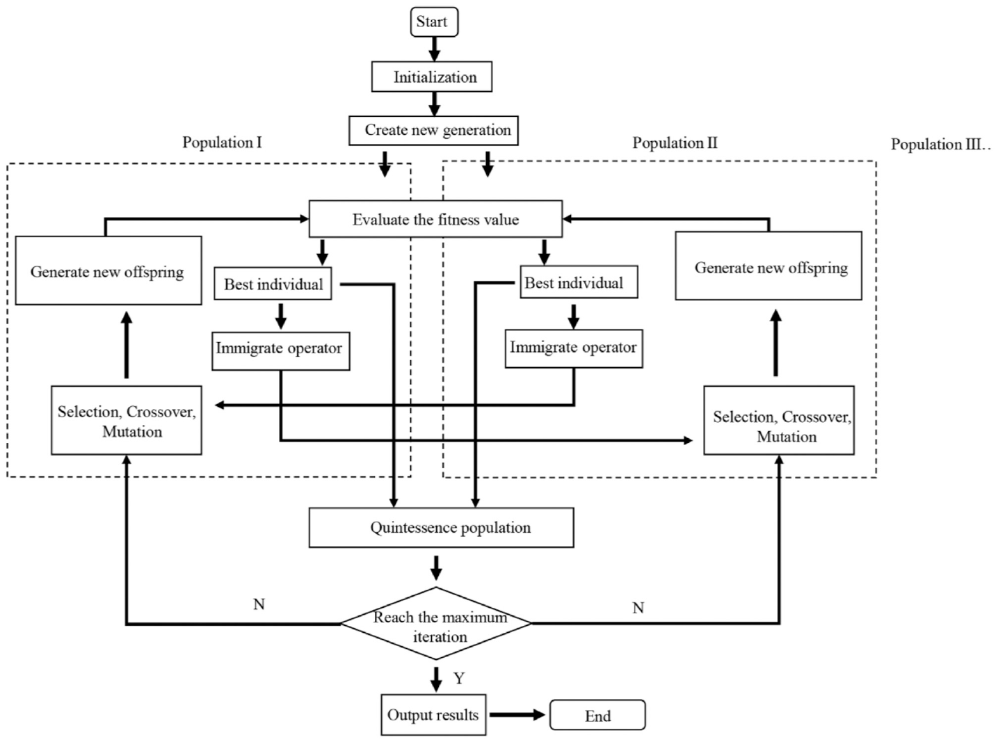
The flowchart of the MPGA.
The training data of the optimization are chosen from the measured restoring forces of the three different configurations of the system: Case (5) d = 0.0587 m, h = 0.0187 m; Case (6) d = 0.0502 m, h = 0.0162 m; Case (7) d = 0.0372 m, h = 0.0162 m, which make the system exhibit mono-stable, bi-stable, and tri-stable stability state, respectively. The main reason for choosing the configuration cases different from Cases (1) to (4) is to prevent the local minima problem to happen in optimization. In this way, it will guarantee that the optimized model is able to predict any configuration in the system’s parameters region. The parameters to be optimized for the first model are chosen to be

and the fitness function used in the optimization for the second model is defined as
where
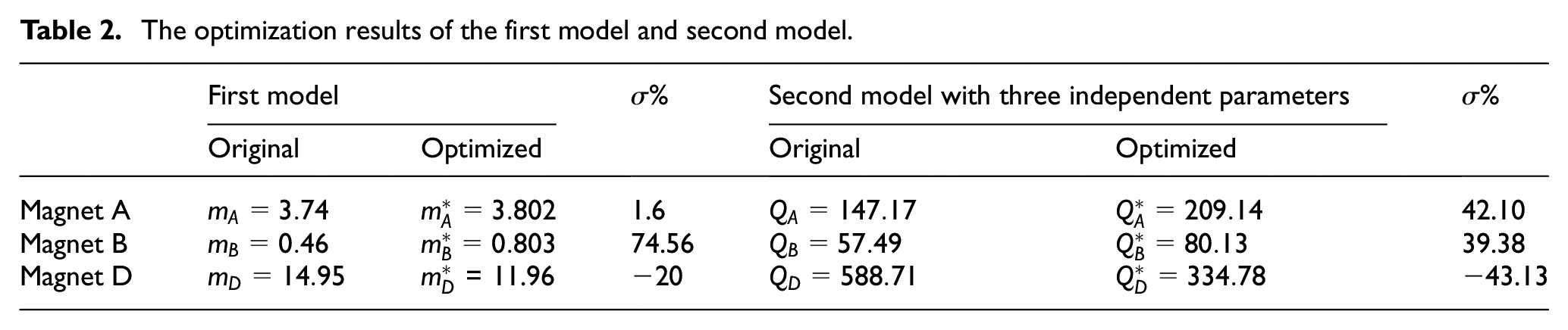
Table 2 lists the optimization results where the differences between the original values and the optimized values are represented by
The optimization results of the first model and second model.
Using the optimum parameters, the simulations of the restoring forces for Cases (1), (2), (3), and (4) are conducted, and the results are shown in Figure 9. The blue dashed lines and red solid lines represent the values of the restoring force based on the optimized first model and the optimized second model, respectively. It can be seen that both optimized models fit the measured values well for all four cases. Table 3 gives a quantitative comparison of the fitness values for the four cases. It can be seen that the fitness value for the first model is drastically reduced and becomes slightly smaller than the fitness value for the second model. Clearly, the proposed optimization significantly improves the accuracy of the first model.
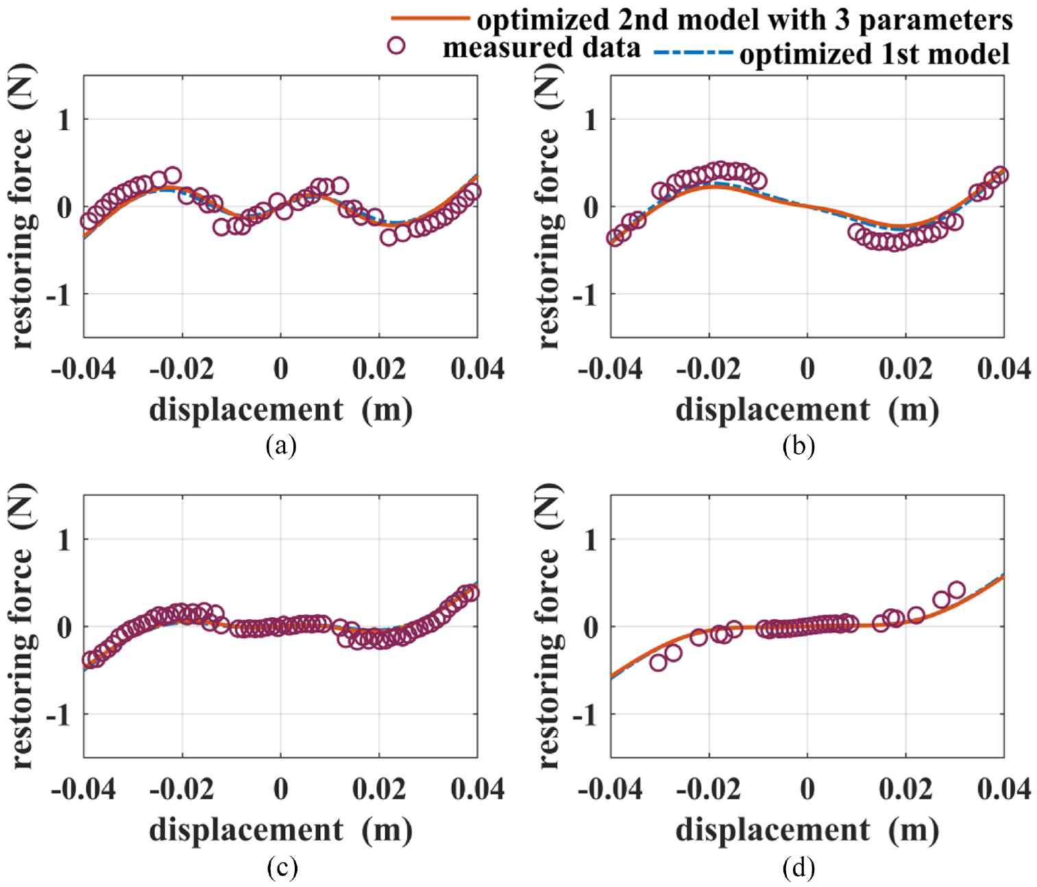
The total restoring forces for: (a) Case (1), (b) Case (2), (c) Case (3), and (d) Case (4) based on the optimized models.
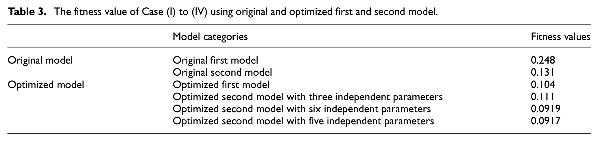
The fitness value of Case (I) to (IV) using original and optimized first and second model.
The above optimization indicates that both optimum models offer a comparable accuracy for the prediction of the restoring forces. As the second approach treats a magnet as a 2-point dipole, it provides more freedom for controlling the model accuracy. One of the possible ways to further improve the model accuracy is to consider all the total charges
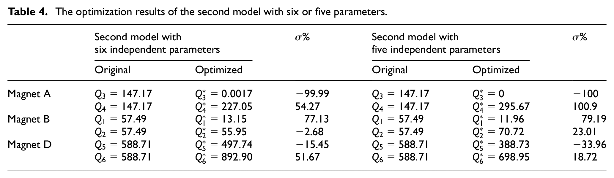
The optimization results of the second model with six or five parameters.
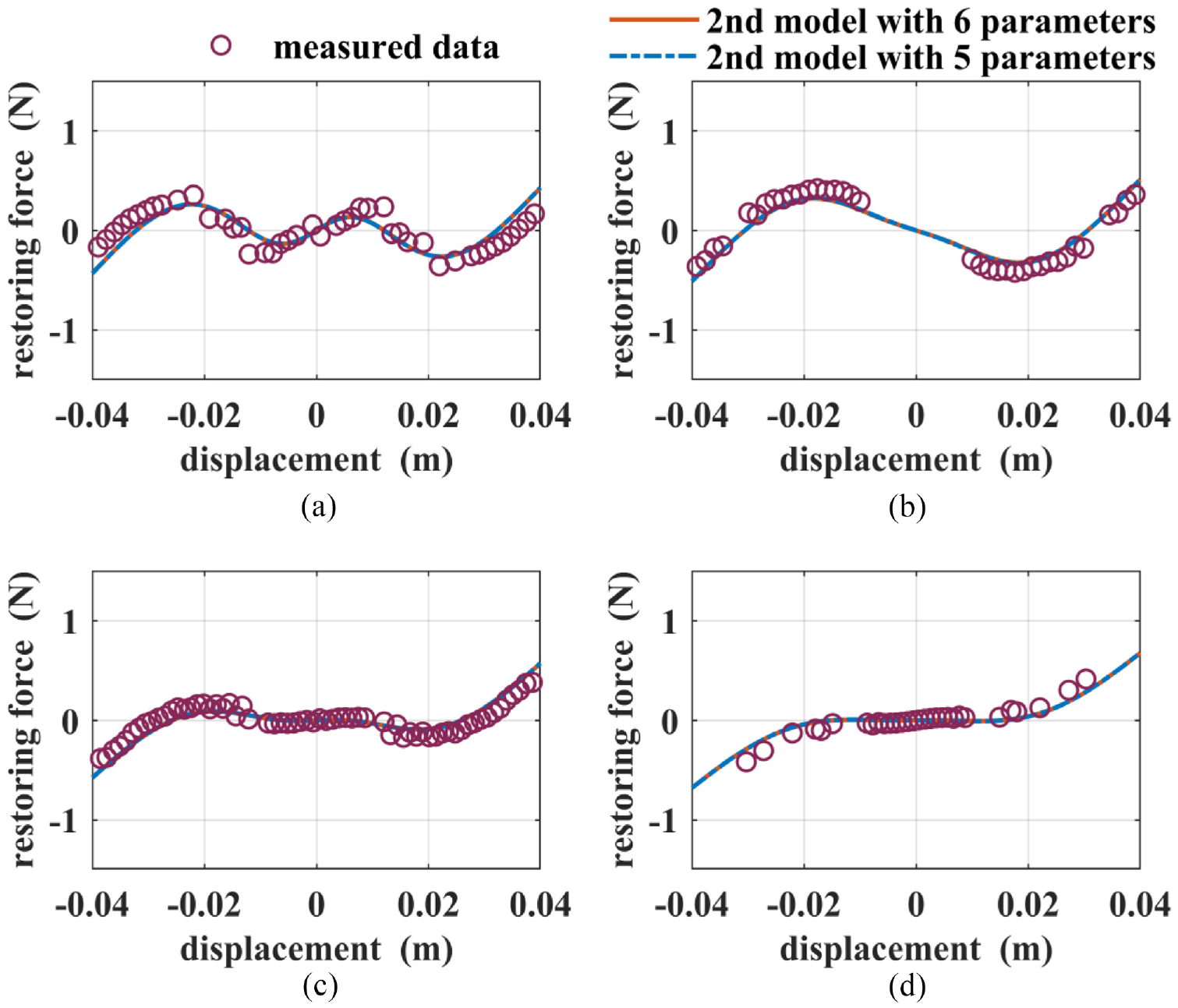
The total restoring forces for: (a) Case (1), (b) Case (2), (c) Case (3), and (d) Case (4) based on the optimized second models with six and five independent parameters.
6. The parametric sensitivity study and stability state region
The sensitivity study intends to evaluate the model robustness against parametric variation. For this purpose, each of the three parameters in the optimum first model and the optimum second model with three parameters is perturbated by
where

where
Errors for Cases (5), (6), and (7) of the optimum first and second models with detuned parameters.
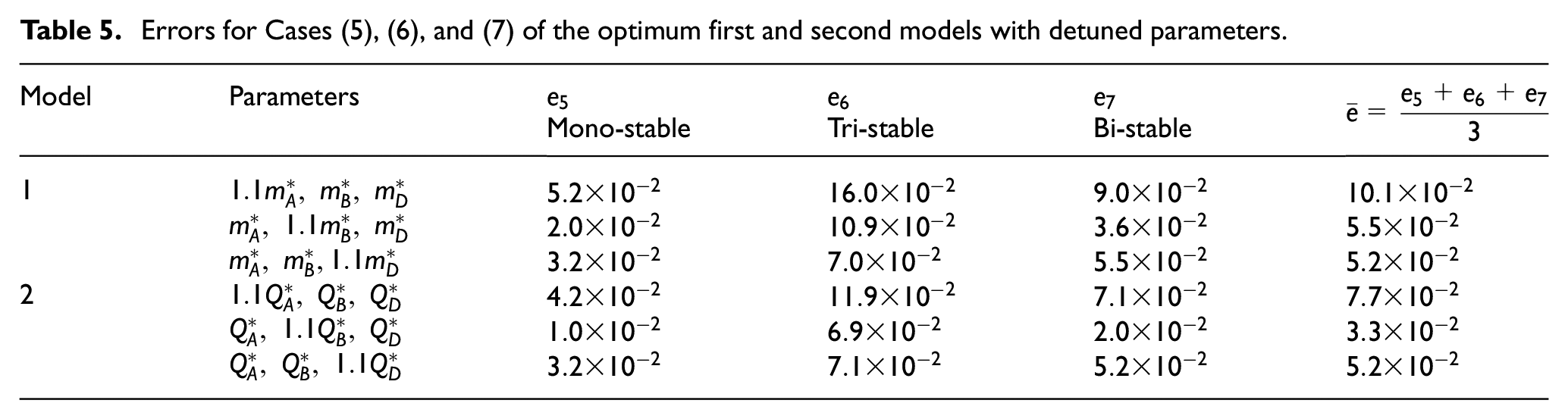
Figures 11 and 12 shows the restoring forces values based on the optimum models and perturbated model. The blue lines represent the restoring forces of the optimum first model or second model, and the red, yellow, and purple lines are the restoring forces of both models when varying the parameters of magnet A, magnet B, and magnet D, respectively. The figures confirm the observations made above. The figures also show the effect of the parameter variation on the trends of the restoring forces. As shown in Figures 11(a), (b) and 12(a), (b), an increase in
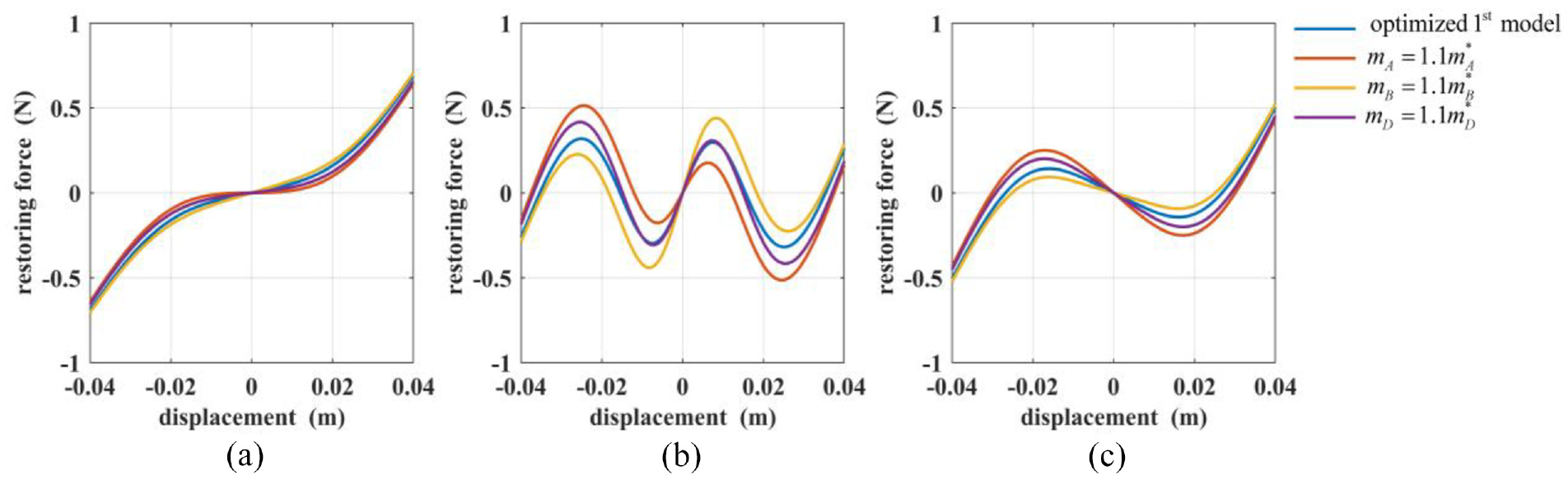
The total restoring forces of the optimized and perturbated first model for: (a) Case (5), (b) Case (6), and (c) Case (7).
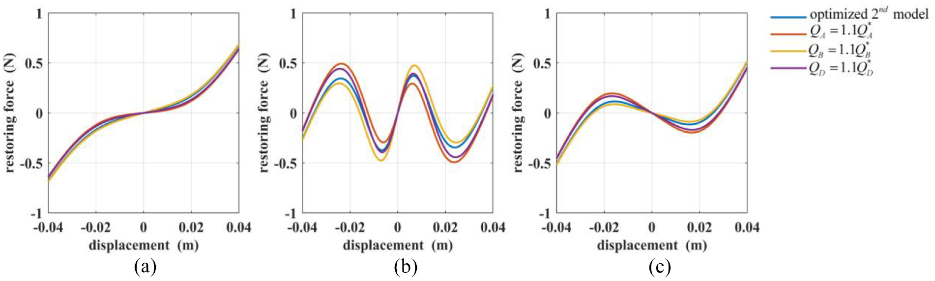
The total restoring forces of the optimized and perturbated second model for: (a) Case (5), (b) Case (6), and (c) Case (7).
With the optimum models, the so-called stability state region can be generated by varying the tuning parameters
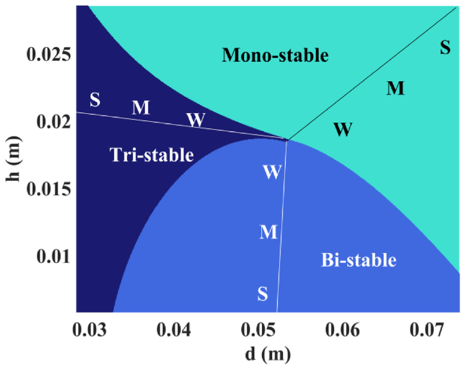
Stability state region.
7. Conclusions
In this study, a tunable multi-stable piezoelectric energy harvester has been developed for applications in an ambient vibration environment with a broad frequency band. The apparatus can be manually tuned to achieve tri-stable, bi-stable, and mono-stable stability states. The magnetic restoring forces of the apparatus have been derived by using two approaches named as first model and second model, respectively. An experimental validation of both models has been conducted. It has been found that although the second model is more accurate than the first model, it has its own limitation. A model optimization has been carried out by using the multi-population genetic algorithm (MPGA). The magnitudes of the magnetic vectors and the amounts of the surface charges of the three magnets have been chosen as parameters to be optimized for the first and second model, respectively. The results show that two optimum models can achieve almost the same level of accuracy. The results also show that the optimum second model has a larger error in predicting the restoring force of the bi-stable state case than the optimum first model. To further improve the accuracy of the second model, the six-parameter optimization has been carried out by assuming that the two surface charges of an individual magnet are different. The results show that the accuracy of the second model with six independent parameters can be further improved. The results also show that the optimum value of
Footnotes
Declaration of conflicting interests
The author(s) declared no potential conflicts of interest with respect to the research, authorship, and/or publication of this article.
Funding
The author(s) disclosed receipt of the following financial support for the research, authorship, and/or publication of this article: This research was financially supported by Natural Sciences and Engineering Council of Canada Discovery Grants (RGPIN/04419-2016).