Multiscale modeling of ferroelectrics with stochastic grain size distribution

Abstract

Macroscopic properties of ferroelectrics are controlled by processes on the microscale, in particular the switching of crystal unit cells and the movement of domain walls, respectively. Besides these microscopic levels, the grains of a polycrystalline material constitute the mesoscopic scale. Interactions of grains with statistically distributed orientations, as a consequence of mechanical and electrostatic mismatch, give rise to for example, residual stress which in turn affects domain switching. A multiscale modeling thus has to incorporate at least three interacting scales. In this context, the condensed method has recently been elaborated as an efficient tool with low computational cost and effort of implementation. It is extended toward statistical distributions of grain sizes in a representative material volume element and amended with regard to the modeling of domain evolution. Each of the few parameters of the constitutive approach has a unique physical meaning and is adapted to available experimental values of macroscopic quantities of barium titanate taken from various sources.

1. Introduction

The class of so-called smart materials nowadays ranges from magnetostrictives and shape memory alloys to electro- or magnetoactive polymers and ferroelectrics. The latter belonging to the wider class of piezoelectrics and being characterized by the capability of switching spontaneous polarization, still play a crucial role herein, combining large stiffness and actuation power with distinguished responsivity. The nonlinear constitutive behavior of ferroelectrics, often illustrated by so-called butterfly hysteresis loops or those of electric displacement versus electric field, has extensively been investigated in the past both theoretically (Chen and Lynch, 1998; Cocks and McMeeking, 1999; Huber and Fleck, 2001; Huber et al., 1999; Hwang and McMeeking, 1998; Hwang et al., 1995, 1998; Kessler and Balke, 2001) and experimentally (Förderreuther, 2003; Franzbach et al., 2014; Huan et al., 2014; Mauck and Lynch, 2003; Wang and Li, 2020) to name only a few of the outstanding works. To validate constitutive models or identify model parameters, the maximum of strain and polarization versus electric field and the respective remanent values are essentially taken as a basis.

Appropriate constitutive models of ferroelectrics have to account for processes on different scales. In particular microphysically motivated models, which largely abstain from phenomenological parameters recorded on an engineering scale, have to account for the switching of crystal unit cells and the resulting movement of domain walls. Since only the latter can be observed under an optical microscope, however, both processes are assigned to different scales, that is, micro- and mesoscale. Another feature of the mesoscale in a polycrystalline material is its grain structure. Exhibiting statistically distributed orientations of crystalline axes and exposed to electromechanical loading, a mismatch of strain and polarization is observed at the grain boundaries. The resulting interaction gives rise to i. a. residual stress which, in turn, has an impact on domain switching. On the macroscopic scale, a representative volume element ( $\mathcal{R}\mathcal{V}\mathcal{E}$ ), containing a sufficiently large number of grains, yields the quantities being of interest for engineering analyses.

The first contributions to homogenization techniques probably trace back to the works of Voigt (1889) and Reuss (1929). More advanced analytical homogenization methods are, for example, the Mori–Tanaka method (Mori and Tanaka, 1973), the differential scheme (Norris, 1985), the self-consistent method (Hill, 1965; Kröner, 1958) or Hashin–Shtrikman type formulations (Hashin and Shtrikman, 1962a, 1962b). However, these analytical approaches have their focus on the calculation of effective moduli of nonhomogeneous materials, rather than providing a coupled multiscale analysis. Numerical homogenization approaches are, for example, the FE2-method, introduced by Smit et al. (1998) and extended toward multiphysical material behavior, for example, by Schröder and Keip (2012), Labusch et al. (2014, 2019) or Uetsuji et al. (2008, 2012, 2019), or FE–FFT based methods (Kochmann et al., 2016; Moulinec and Suquet, 1998). Semi-analytical methods have recently been applied to multiscale problems, for example, by Wulfinghoff et al. (2018) or Jaworek et al. (2020), where an analytical homogenization procedure for the microscopic boundary value problem and thus for each Gauss point is considered within a FE framework.

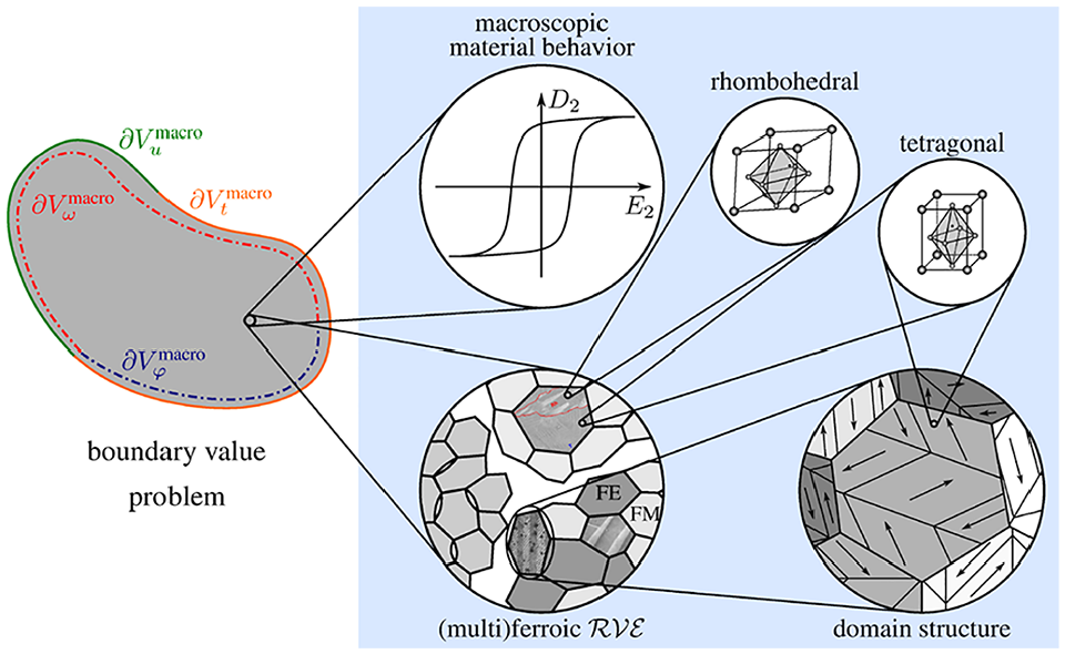
Figure 1 illustrates multiscale modeling features of ferroic functional materials, where the macroscopic mixed boundary value problem is depicted on the left hand side, whereas the blue box on the right comprises aspects of different scales. An $\mathcal{R}\mathcal{V}\mathcal{E}$ represents a macroscopic material point and can involve grains of different compositions and for example, microcracks. Ferroelectric grains exhibit mesostructures with for example, $90°$ and $180°$ domain walls in a tetragonal phase. Unit cells, in turn, constitute the domains, whereat different types may basically coexist in one grain, for example, for morphotropic compositions of PZT ceramics.

Figure 1.

Multiscale aspects of ferroic functional materials with ferroelectric (FE) or ferromagnetic (FM) grains and domain patterns on the mesoscale, tetragonal, and rhombohedral unit cells on the microscale and a dielectric hysteresis loop representing local macroscopic constitutive behavior of a boundary value problem. Micrographs of the domain structures are taken from Arlt (1990b), Egelkamp and Reimer (1990), and Scholehwar (2010).

In the recent past, all these aspects have been included in modeling approaches of ferroelectric, ferromagnetic, and multiferroic materials, based on the so-called condensed method (CM) (Behlen et al., 2021; Lange and Ricoeur, 2015, 2016; Ricoeur and Lange, 2019; Uckermann et al., 2018; Warkentin and Ricoeur, 2020). This semi-analytical approach comprises homogenization within a multiphysical framework and scale–bridging interactions in a simple but robust and thermodynamically and electromechanically consistent manner. Its implementation is straightforward and results of $\mathcal{R}\mathcal{V}\mathcal{E}$ s are obtained with comparatively low computational cost. In comparison to most of the above mentioned multiscale approaches, the CM is able to calculate macroscopic as well as microscopic quantities without any kind of discretization scheme.

This work pursues two objectives. The model of tetragonal ferroelectrics developed in the context of the CM is extended at two points. Rhombohedral and ferromagnetic systems, as indicated in Figure 1, are not considered here, however, could straightforwardly be included in the extensions. In the averaging approach grains have hitherto been considered as equally sized, which is now replaced by an assumption of Gaussian distribution. The stochastic nature of the problem is thus incorporated twofold now, that is, in terms of grain orientation and relative size. The absolute sizes distinguishing fine and coarse grained behaviors in terms of different hierarchical domain levels, effects on lattice parameters (Huan et al., 2014; Li and Wang, 2017) or influences on material properties, see for example, Tan et al. (2015), are disregarded at this point. Another extension of the model introduces a lower limit for magnitudes of internal variables representing volume fractions of domains in a grain. Physically, it ensures that moving domain walls are not allowed to vanish due to external loading. Introducing an additional parameter on the one hand side, it replaces two tuning parameters on the other, which have hitherto been included in the constitutive equations to reduce switching strain and polarization.

The second objective of the work is to adapt essential parameters of the model to experimental findings of barium titanate (BT) as an exemplary material and to demonstrate the quantitative appropriateness of the modeling approach. In this context, experiments turn out to yield a considerable range of relevant quantities which is recorded compiling available hystereses of strain and electric displacement versus electric field. Predicted remanent and maximum values of strain and electric displacement are compared to the respective experimental ranges. The studies target accuracy just as computational costs, partly constituting competing factors. Residual stress is finally investigated due to its relevance for strength and reliability of the brittle ceramics.

2. Constitutive framework of a ferroelectric grain

The thermodynamic potential of the considered nonlinear ferroelectric material behavior reads, see for example, Wingen and Ricoeur (2019) or Ricoeur and Lange (2019):

$$\begin{array}{c}{\mathrm{\Psi }}_{\mathrm{em}}({\epsilon }_{\mathrm{kl}},E_l)=\frac{1}{2}{C}_{\mathrm{ijkl}}{\epsilon }_{\mathrm{ij}}{\epsilon }_{\mathrm{kl}}-\frac{1}{2}{\kappa }_{\mathrm{il}}{E}_i{E}_l-e_{\mathrm{lij}}{\epsilon }_{\mathrm{ij}}{E}_l-\hfill \\ -(C_{\mathrm{ijkl}}{\epsilon }_{\mathrm{kl}}-e_{\mathrm{lij}}{E}_l){\epsilon }_{\mathrm{ij}}^{\mathrm{irr}}-\frac{1}{2}{C}_{\mathrm{ijkl}}{\epsilon }_{\mathrm{ij}}^{\mathrm{irr}}{\epsilon }_{\mathrm{kl}}^{\mathrm{irr}}-E_l{P}_l^{\mathrm{irr}}.\hfill \end{array}$$

(1)

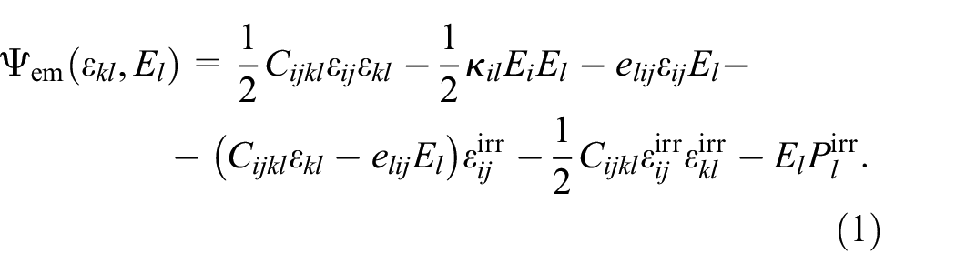
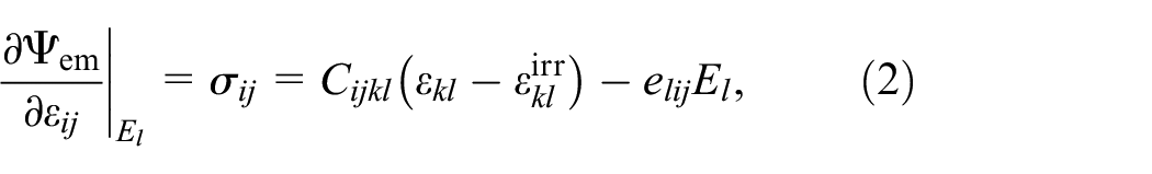
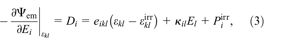
In equation (1) $C_{\mathrm{ijkl}}$ , $e_{\mathrm{lij}}$ , and ${\kappa }_{\mathrm{il}}$ describe the elastic, piezoelectric and dielectric properties and ${\epsilon }_{\mathrm{kl}}^{\mathrm{irr}}$ and $P_i^{\mathrm{irr}}$ denote irreversible contributions due to domain wall motion. The independent variables within the constitutive framework are ${\epsilon }_{\mathrm{kl}}$ and $E_l$ . The partial derivatives of equation (1), with respect to the independent variables, lead to the constitutive equations, see for example, Lange and Ricoeur (2015),

$${\frac{\partial {\mathrm{\Psi }}_{\mathrm{em}}}{\partial {\epsilon }_{\mathrm{ij}}}|}_{E_l}={\sigma }_{\mathrm{ij}}=C_{\mathrm{ijkl}}({\epsilon }_{\mathrm{kl}}-{\epsilon }_{\mathrm{kl}}^{\mathrm{irr}})-e_{\mathrm{lij}}{E}_l,$$

(2)

$$-{\frac{\partial {\mathrm{\Psi }}_{\mathrm{em}}}{\partial E_i}|}_{{\epsilon }_{\mathrm{kl}}}=D_i=e_{\mathrm{ikl}}({\epsilon }_{\mathrm{kl}}-{\epsilon }_{\mathrm{kl}}^{\mathrm{irr}})+{\kappa }_{\mathrm{il}}{E}_l+P_i^{\mathrm{irr}},$$

(3)

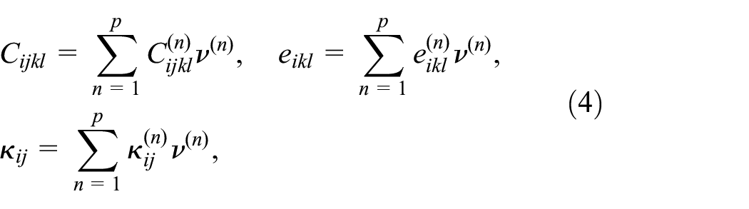
where ${\sigma }_{\mathrm{ij}}$ and $D_i$ denote the associated variables mechanical stress and electric displacement. In equations (2) and (3) the material properties of a grain have been assumed constant in incremental changes of state and are determined as weighted averages, see for example, Avakian and Ricoeur (2016) or Huber et al. (1999),

$$\begin{array}{c}{C}_{\mathrm{ijkl}}=\sum _{n=1}^p{C}_{\mathrm{ijkl}}^{(n)}{\nu }^{(n)},e_{\mathrm{ikl}}=\sum _{n=1}^p{e}_{\mathrm{ikl}}^{(n)}{\nu }^{(n)},\hfill \\ {\kappa }_{\mathrm{ij}}=\sum _{n=1}^p{\kappa }_{\mathrm{ij}}^{(n)}{\nu }^{(n)},\hfill \end{array}$$

(4)

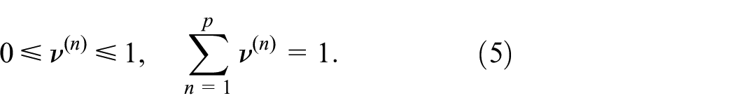
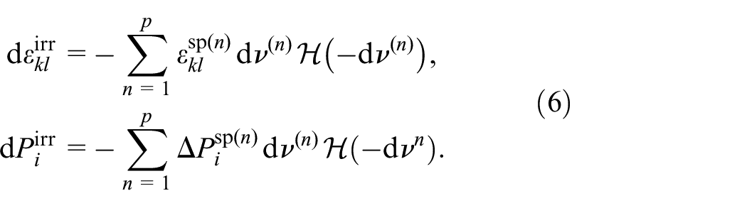
where domains with homogeneous material properties are assumed and $p$ is associated with the number of domain variants per grain. In equation (4) $C_{\mathrm{ijkl}}^{(n)}$ , $e_{\mathrm{ikl}}^{(n)}$ , ${\kappa }_{\mathrm{ij}}^{(n)}$ represent the elastic, piezoelectric, and dielectric coefficients of the domain $n$ . Ferroelectric materials with tetragonal unit cells exhibit a domain structure with $90°$ and $180°$ domain walls, which is depicted in Figure 2. On the right hand side the motivations for the micromechanical model and the internal variables ${\nu }^{(n)}$ are given. The 3D domain structure of a grain is represented by a microscopic material point (MiMP) with six possible polarization directions, that is, $p=6$ . Each direction is weighted by ${\nu }^{(n)}$ , where $n=1,\dots ,p$ . Following the work of Huber et al. (1999), the internal variables are interpreted as volume fractions of the domain species and have to satisfy the following conditions:

$$0\le {\nu }^{(n)}\le 1,\sum _{n=1}^p{\nu }^{(n)}=1.$$

(5)

Figure 2.

Left: three-dimensional domain structure of a ferroelectric grain with tetragonal unit cells (in the style of Arlt, 1990a); right: motivation of the micromechanical model with six prevailing directions of spontaneous polarization $P_i^{\mathrm{sp}(n)}$ .

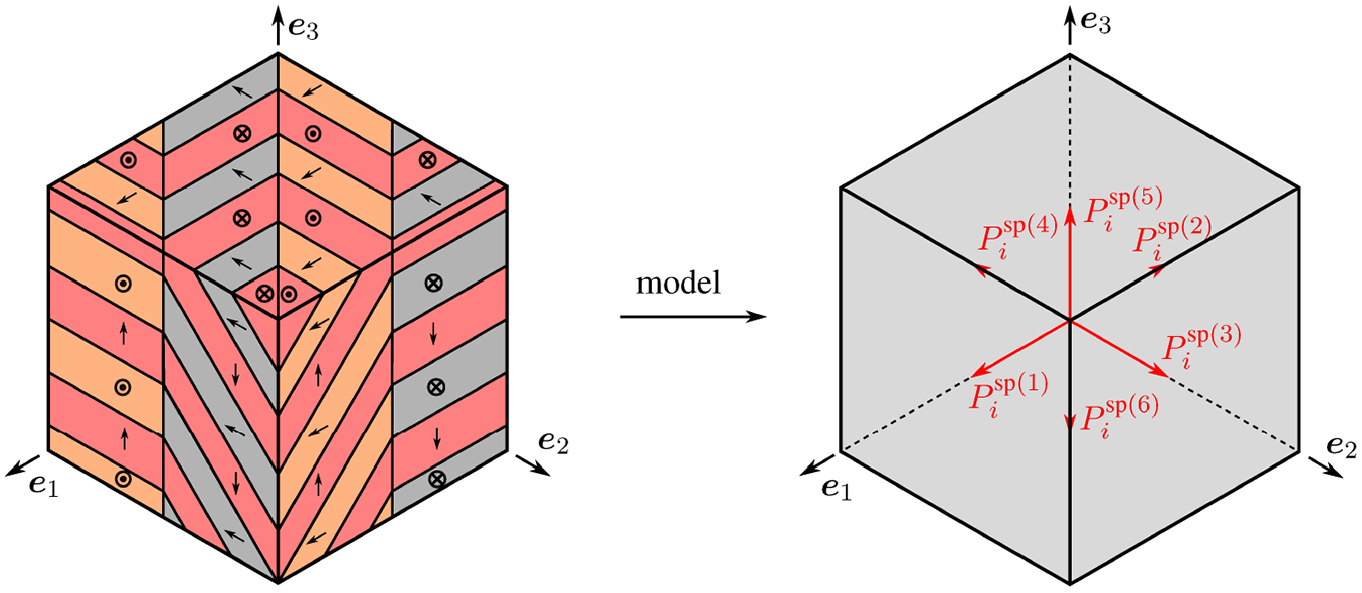
The evolution of the irreversible contributions is obtained as follows (Ricoeur and Lange, 2019):

$$\begin{array}{cc}\multicolumn{1}{c}{\mathrm{d}{\epsilon }_{\mathrm{kl}}^{\mathrm{irr}}}& =-\sum _{n=1}^p{\epsilon }_{\mathrm{kl}}^{\mathrm{sp}(n)}\mathrm{d}{\nu }^{(n)}\mathcal{H}(-\mathrm{d}{\nu }^{(n)}),\hfill \\ \multicolumn{1}{c}{\mathrm{d}{P}_i^{\mathrm{irr}}}& =-\sum _{n=1}^p\mathrm{\Delta }{P}_i^{\mathrm{sp}(n)}\mathrm{d}{\nu }^{(n)}\mathcal{H}(-\mathrm{d}{\nu }^n).\hfill \end{array}$$

(6)

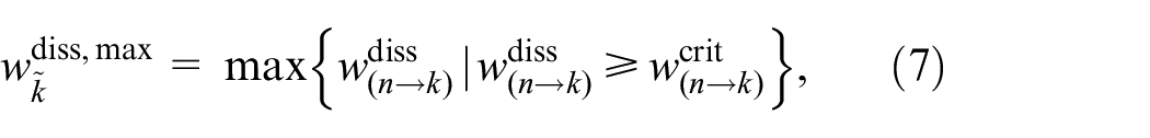
The spontaneous strain ${\epsilon }_{\mathrm{kl}}^{\mathrm{sp}(n)}$ is induced by $90°$ switching domains, whereas the change of spontaneous polarization $\mathrm{\Delta }{P}_i^{\mathrm{sp}(n)}$ depends on the kind of switching, see Appendix. The HEAVISIDE-functions $\mathcal{H}(-\mathrm{d}{\nu }^{(n)})$ take the value 1 for domain species $n$ which are switching, thus reducing the associated internal variables, and 0 for those being enriched by the switching. In equation (6) $\mathrm{d}{\nu }^{(n)}$ describes the change of the volume fraction ${\nu }^{(n)}$ , see Figure 2, for a switching process from domain variant $n$ to domain species $\tilde{k}$ , where the latter is associated with the maximum energy dissipation

$$w_{\tilde{k}}^{\mathrm{diss},\max }=max\{w_{(n\to k)}^{\mathrm{diss}}|w_{(n\to k)}^{\mathrm{diss}}\ge w_{(n\to k)}^{\mathrm{crit}}\},$$

(7)

which satisfies the necessary condition of exceeding a threshold $w_{(n\to k)}^{\mathrm{crit}}$ .

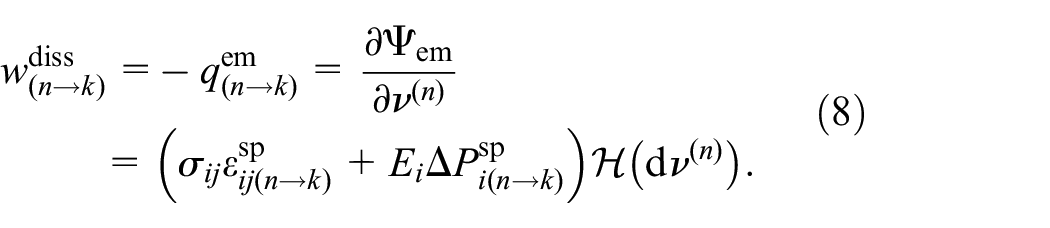
The dissipative work $w_{(n\to k)}^{\mathrm{diss}}$ of a switching process from domain species $n$ to $k$ is equal to the negative thermodynamic driving force $q_{(n\to k)}^{\mathrm{em}}$ and is thus obtained from the potential equation (1) by differentiation with respect to the internal variable (Wingen and Ricoeur, 2019):

$$\begin{array}{c}{w}_{(n\to k)}^{\mathrm{diss}}=-q_{(n\to k)}^{\mathrm{em}}=\frac{\partial {\mathrm{\Psi }}_{\mathrm{em}}}{\partial {\nu }^{(n)}}\hfill \\ =({\sigma }_{\mathrm{ij}}{\epsilon }_{\mathrm{ij}(n\to k)}^{\mathrm{sp}}+E_i\mathrm{\Delta }{P}_{i(n\to k)}^{\mathrm{sp}})\mathcal{H}\left(\mathrm{d}{\nu }^{(n)}\right).\hfill \end{array}$$

(8)

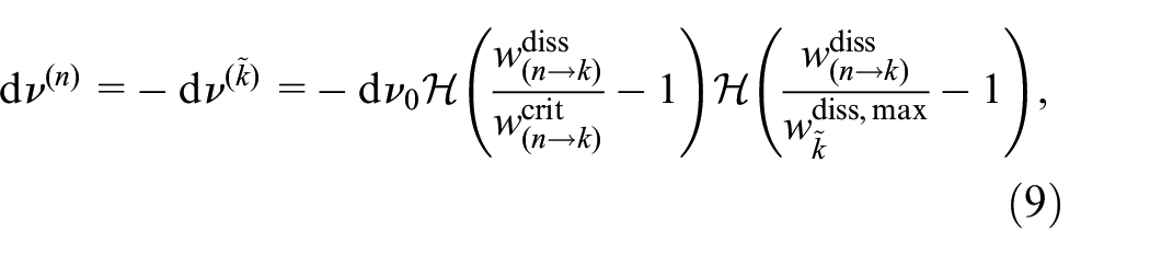
It should be mentioned, that equation (8) neglects the dependence of the material coefficients on the internal variables. An extension for the dissipative work was suggested by Kessler and Balke (2001) taking into account higher order effects. The dissipative work, outlined in equation (8), was originally introduced in the switching criterion by Hwang et al. (1995). A more detailed derivation of $w_{(n\to k)}^{\mathrm{diss}}$ is found in Ricoeur and Lange (2019). The evolution law for the internal variables ${\nu }^{(n)}$ is formulated as follows:

$$\mathrm{d}{\nu }^{(n)}=-\mathrm{d}{\nu }^{(\tilde{k})}=-\mathrm{d}{\nu }_0\mathcal{H}(\frac{w_{(n\to k)}^{\mathrm{diss}}}{w_{(n\to k)}^{\mathrm{crit}}}-1)\mathcal{H}(\frac{w_{(n\to k)}^{\mathrm{diss}}}{w_{\tilde{k}}^{\mathrm{diss},\max }}-1),$$

(9)

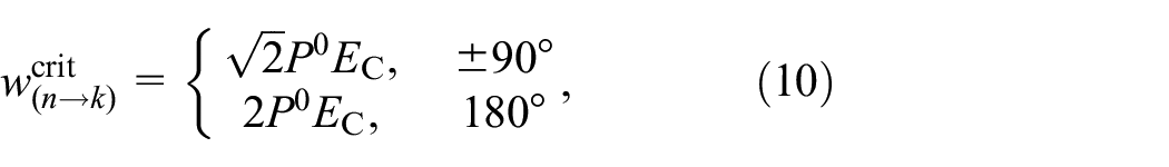
where $\mathrm{d}{\nu }_0$ is a model parameter and the HEAVISIDE-functions as usual take the value 1 for a positive argument including 0, and 0 for a negative value. The first HEAVISIDE-function in equation (9) verifies, if switching from domain $n$ to $k$ is feasible, whereas the second ensures that the one switching process from domain $n$ to domain $\tilde{k}$ associated with the maximum energy dissipation takes place. The energy threshold $w_{(n\to k)}^{\mathrm{crit}}$ depends on the type of switching. For ferroelectric materials with tetragonal unit cells, motions of $90°$ and $180°$ domain walls are possible. Hence, the energy threshold reads, see for example, Hwang et al. (1995) and Huber et al. (1999):

$$w_{(n\to k)}^{\mathrm{crit}}=\{\begin{array}{cc}\sqrt{2}{P}^0{E}_{\mathrm{C}},\hfill & \pm 90°\hfill \\ \multicolumn{1}{c}{2P^0{E}_{\mathrm{C}},}& 180°\hfill \end{array},$$

(10)

where $P^0$ and $E_{\mathrm{C}}$ denote the spontaneous polarization and the coercive field, respectively, see Table A2.

The range of the internal variables outlined in equation (5) implies, that domains can vanish in favor of other domains. From a physical point of view, this behavior is inappropriate since domain walls are indispensable for the reduction of potential energy in a grain. Allowing for unconstrained switching within in the limits of equation (5) gives rise to an overestimation of the irreversible contributions ${\epsilon }_{\mathrm{kl}}^{\mathrm{irr}}$ and $P_i^{\mathrm{irr}}$ . In Gellmann and Ricoeur (2016) or Lange and Ricoeur (2015) two additional parameters have been introduced in the constitutive equations to face this deficiency and eventually meet experimental results. Within FE-frameworks it was further required for numerical stability. A more physically motivated approach is the implementation of a lower limit ${\nu }_{\min }$ for the volume fractions, thus adapting the range of the internal variables according to

$${\nu }_{\min }<{\nu }^{(n)}<1.$$

(11)

Since ${\nu }_{\min }>0$ it is guaranteed that domains of a MiMP and grain, respectively, cannot vanish. This improved approach introduces just one additional parameter which helps adapting numerical to experimental results. The second model parameter $\mathrm{d}{\nu }_0$ of equation (9) just has to be chosen sufficiently small to attain convergence.

3. Micro–macro–transition with variable grain size

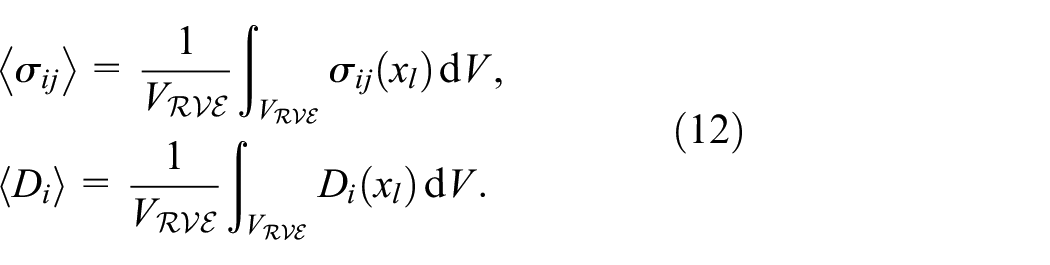
On the macroscopic scale, represented by an $\mathcal{R}\mathcal{V}\mathcal{E}$ , quantities, for example, mechanical stress ${\sigma }_{\mathrm{ij}}$ and electric displacement $D_i$ , are microscopic volume averages, see for example, Hori and Nemat-Nasser (1998) or Kessler and Balke (2001):

$$\begin{array}{c}〈{\sigma }_{\mathrm{ij}}〉=\frac{1}{V_{\mathcal{R}\mathcal{V}\mathcal{E}}}{\int }_{V_{\mathcal{R}\mathcal{V}\mathcal{E}}}{\sigma }_{\mathrm{ij}}\left(x_l\right)\mathrm{d}V,\hfill \\ 〈D_i〉=\frac{1}{V_{\mathcal{R}\mathcal{V}\mathcal{E}}}{\int }_{V_{\mathcal{R}\mathcal{V}\mathcal{E}}}{D}_i\left(x_l\right)\mathrm{d}V.\hfill \end{array}$$

(12)

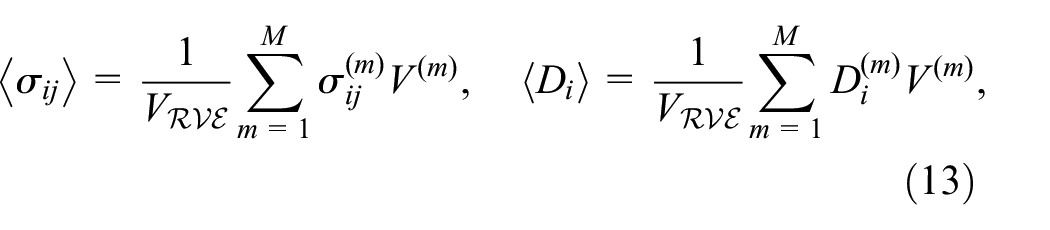
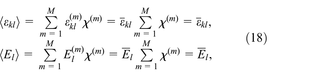
In equation (12) and in the following, macroscopic quantities, obtained by homogenization, are specified by angled brackets. Assuming, homogeneous fields in a MiMP $m$ with the volume $V^{(m)}$ , that is, ${\sigma }_{\mathrm{ij}}^{(m)},D_i^{(m)}=\mathrm{const}$ in $V^{(m)}$ , the volume averages are given as

$$〈{\sigma }_{\mathrm{ij}}〉=\frac{1}{V_{\mathcal{R}\mathcal{V}\mathcal{E}}}\sum _{m=1}^M{\sigma }_{\mathrm{ij}}^{(m)}{V}^{(m)},〈D_i〉=\frac{1}{V_{\mathcal{R}\mathcal{V}\mathcal{E}}}\sum _{m=1}^M{D}_i^{(m)}{V}^{(m)},$$

(13)

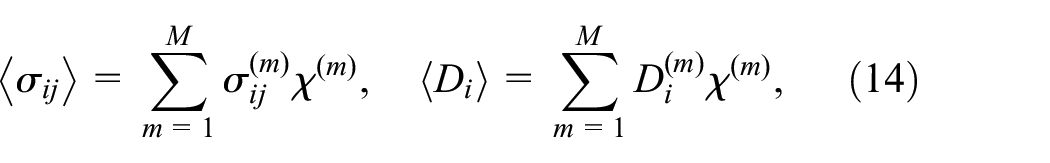
where $M$ denotes the number of grains in the $\mathcal{R}\mathcal{V}\mathcal{E}$ . In contrast to Lange and Ricoeur (2015) and Ricoeur and Lange (2019), where $V_{\mathcal{R}\mathcal{V}\mathcal{E}}=M{V}^{(m)}$ has been considered, MiMPs and thus grains of the $\mathcal{R}\mathcal{V}\mathcal{E}$ do not hold equal sizes now. Macroscopic quantities, outlined in equations (12) and (13), finally read

$$〈{\sigma }_{\mathrm{ij}}〉=\sum _{m=1}^M{\sigma }_{\mathrm{ij}}^{(m)}{\chi }^{(m)},〈D_i〉=\sum _{m=1}^M{D}_i^{(m)}{\chi }^{(m)},$$

(14)

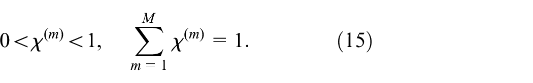
where ${\chi }^{(m)}=V^{(m)}/V_{\mathcal{R}\mathcal{V}\mathcal{E}}$ describes the volume fraction of the MiMP $m$ . Similar to the volume fraction of a domain ${\nu }^{(n)}$ , all ${\chi }^{(m)}$ have to satisfy the following conditions:

$$0<{\chi }^{(m)}<1,\sum _{m=1}^M{\chi }^{(m)}=1.$$

(15)

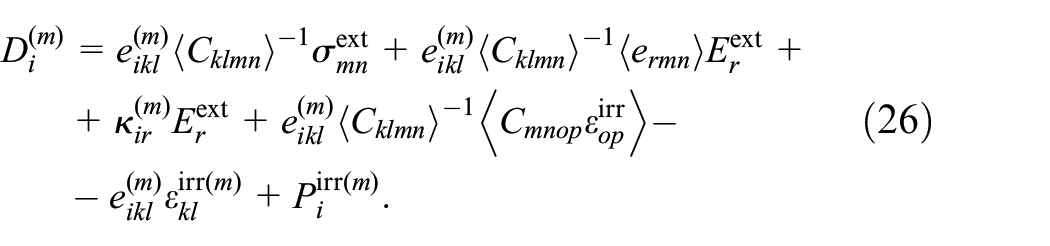
Inserting equations (2) and (3) into equation (14), macroscopic stress and electric displacement are obtained as follows:

$$〈{\sigma }_{\mathrm{ij}}〉=\sum _{m=1}^M(C_{\mathrm{ijkl}}^{(m)}({\epsilon }_{\mathrm{kl}}^{(m)}-{\epsilon }_{\mathrm{kl}}^{\mathrm{irr}(m)})-e_{\mathrm{lij}}^{(m)}{E}_l^{(m)}){\chi }^{(m)},$$

(16)

$$〈D_i〉=\sum _{m=1}^M(e_{\mathrm{ikl}}^{(m)}({\epsilon }_{\mathrm{kl}}^{(m)}-{\epsilon }_{\mathrm{kl}}^{\mathrm{irr}(m)})+{\kappa }_{\mathrm{il}}^{(m)}{E}_l^{(m)}+P_i^{\mathrm{irr}(m)}){\chi }^{(m)}.$$

(17)

It should be kept in mind that the constitutive equations of the previous section are interpreted as constitutive equations of a grain $m$ . The material properties $C_{\mathrm{ijkl}}^{(m)}$ , $e_{\mathrm{ikl}}^{(m)}$ , and ${\kappa }_{\mathrm{il}}^{(m)}$ as well as the irreversible contributions ${\epsilon }_{\mathrm{kl}}^{\mathrm{irr}(m)}$ and $P_i^{\mathrm{irr}(m)}$ depend on the internal variables ${\nu }^{(n)}$ , see equations (4) and (6). A generalized Voigt-approximation, that is

$$\begin{array}{c}〈{\epsilon }_{\mathrm{kl}}〉=\sum _{m=1}^M{\epsilon }_{\mathrm{kl}}^{(m)}{\chi }^{(m)}={\overline{\epsilon }}_{\mathrm{kl}}\sum _{m=1}^M{\chi }^{(m)}={\overline{\epsilon }}_{\mathrm{kl}},\hfill \\ \multicolumn{1}{c}{〈E_l〉=\sum _{m=1}^M{E}_l^{(m)}{\chi }^{(m)}={\overline{E}}_l\sum _{m=1}^M{\chi }^{(m)}={\overline{E}}_l,}\end{array}$$

(18)

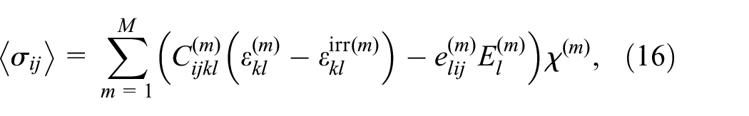
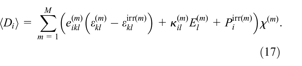
is applied for the sake of a scale transition. The macroscopic constitutive equations (16) and (17) finally read:

$$〈{\sigma }_{\mathrm{ij}}〉=〈C_{\mathrm{ijkl}}〉{\overline{\epsilon }}_{\mathrm{kl}}-〈e_{\mathrm{lij}}〉{\overline{E}}_l-〈C_{\mathrm{ijkl}}{\epsilon }_{\mathrm{kl}}^{\mathrm{irr}}〉,$$

(19)

$$〈D_i〉=〈e_{\mathrm{ikl}}〉{\overline{\epsilon }}_{\mathrm{kl}}+〈{\kappa }_{\mathrm{il}}〉{\overline{E}}_l+〈P_i^{\mathrm{irr}}〉.$$

(20)

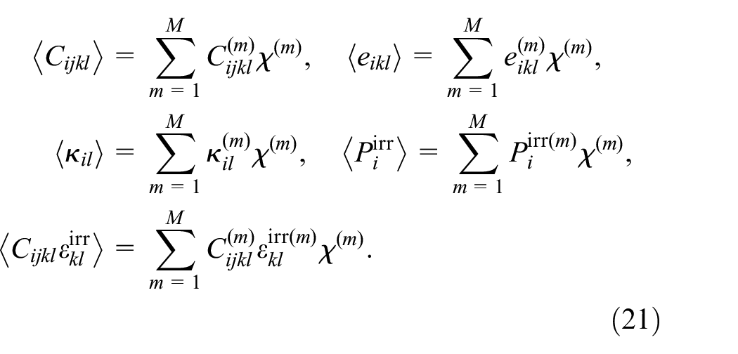
The macroscopic material properties $〈C_{\mathrm{ijkl}}〉$ , $〈e_{\mathrm{ikl}}〉$ , $〈{\kappa }_{\mathrm{il}}〉$ and the inelastic contributions $〈C_{\mathrm{ijkl}}{\epsilon }_{\mathrm{kl}}^{\mathrm{irr}}〉$ and $〈P_i^{\mathrm{irr}}〉$ depend on the volume fractions ${\chi }^{(m)}$ :

$$\begin{array}{cc}\multicolumn{1}{c}{〈C_{\mathrm{ijkl}}〉}& =\sum _{m=1}^M{C}_{\mathrm{ijkl}}^{(m)}{\chi }^{(m)},〈e_{\mathrm{ikl}}〉=\sum _{m=1}^M{e}_{\mathrm{ikl}}^{(m)}{\chi }^{(m)},\hfill \\ \multicolumn{1}{c}{〈{\kappa }_{\mathrm{il}}〉}& =\sum _{m=1}^M{\kappa }_{\mathrm{il}}^{(m)}{\chi }^{(m)},〈P_i^{\mathrm{irr}}〉=\sum _{m=1}^M{P}_i^{\mathrm{irr}(m)}{\chi }^{(m)},\hfill \\ \multicolumn{1}{c}{〈C_{\mathrm{ijkl}}{\epsilon }_{\mathrm{kl}}^{\mathrm{irr}}〉}& =\sum _{m=1}^M{C}_{\mathrm{ijkl}}^{(m)}{\epsilon }_{\mathrm{kl}}^{\mathrm{irr}(m)}{\chi }^{(m)}.\hfill \end{array}$$

(21)

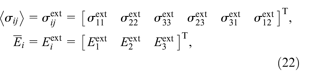
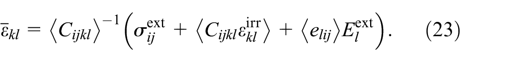
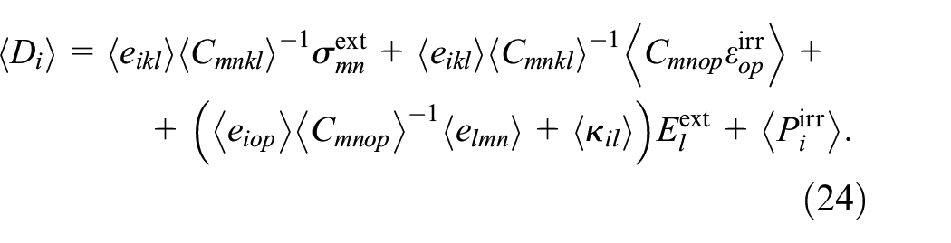
Equations (19) and (20) contain known and unknown quantities of an $\mathcal{R}\mathcal{V}\mathcal{E}$ , depending on the given problem. In particular, these are the macroscopic mechanical stress $〈{\sigma }_{\mathrm{ij}}〉$ , electric displacement $〈D_i〉$ , strain ${\overline{\epsilon }}_{\mathrm{kl}}$ , and electric field ${\overline{E}}_l$ . Prescribing stress and electric field as external loads, that is

$$\begin{array}{cc}\multicolumn{1}{c}{〈{\sigma }_{\mathrm{ij}}〉={\sigma }_{\mathrm{ij}}^{\mathrm{ext}}}& ={\left[\begin{array}{cccccc}{\sigma }_{11}^{\mathrm{ext}}\hfill & {\sigma }_{22}^{\mathrm{ext}}\hfill & {\sigma }_{33}^{\mathrm{ext}}\hfill & {\sigma }_{23}^{\mathrm{ext}}\hfill & {\sigma }_{31}^{\mathrm{ext}}\hfill & {\sigma }_{12}^{\mathrm{ext}}\hfill \end{array}\right]}^{\mathrm{T}},\hfill \\ \multicolumn{1}{c}{{\overline{E}}_i=E_i^{\mathrm{ext}}}& ={\left[\begin{array}{ccc}{E}_1^{\mathrm{ext}}\hfill & E_2^{\mathrm{ext}}\hfill & E_3^{\mathrm{ext}}\hfill \end{array}\right]}^{\mathrm{T}},\hfill \end{array}$$

(22)

the macroscopic strain results from equation (19):

$${\overline{\epsilon }}_{\mathrm{kl}}={〈C_{\mathrm{ijkl}}〉}^{-1}({\sigma }_{\mathrm{ij}}^{\mathrm{ext}}+〈C_{\mathrm{ijkl}}{\epsilon }_{\mathrm{kl}}^{\mathrm{irr}}〉+〈e_{\mathrm{lij}}〉E_l^{\mathrm{ext}}).$$

(23)

Inserting equation (23) in equation (20), the macroscopic electric displacement reads

$$\begin{array}{c}\multicolumn{1}{c}{〈D_i〉=〈e_{\mathrm{ikl}}〉{〈C_{\mathrm{mnkl}}〉}^{-1}{\sigma }_{\mathrm{mn}}^{\mathrm{ext}}+〈e_{\mathrm{ikl}}〉{〈C_{\mathrm{mnkl}}〉}^{-1}〈C_{\mathrm{mnop}}{\epsilon }_{\mathrm{op}}^{\mathrm{irr}}〉+}\\ +(〈e_{\mathrm{iop}}〉{〈C_{\mathrm{mnop}}〉}^{-1}〈e_{\mathrm{lmn}}〉+〈{\kappa }_{\mathrm{il}}〉)E_l^{\mathrm{ext}}+〈P_i^{\mathrm{irr}}〉.\hfill \end{array}$$

(24)

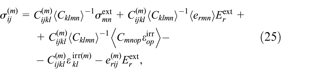
Residual stresses ${\sigma }_{\mathrm{ij}}^{(m)}$ and electric displacement $D_i^{(m)}$ of a grain $m$ are obtained inserting equation (23) in equations (2) and (3):

$$\begin{array}{c}\multicolumn{1}{c}{{\sigma }_{\mathrm{ij}}^{(m)}=C_{\mathrm{ijkl}}^{(m)}{〈C_{\mathrm{klmn}}〉}^{-1}{\sigma }_{\mathrm{mn}}^{\mathrm{ext}}+C_{\mathrm{ijkl}}^{(m)}{〈C_{\mathrm{klmn}}〉}^{-1}〈e_{\mathrm{rmn}}〉E_r^{\mathrm{ext}}+}\\ +C_{\mathrm{ijkl}}^{(m)}{〈C_{\mathrm{klmn}}〉}^{-1}〈C_{\mathrm{mnop}}{\epsilon }_{\mathrm{op}}^{\mathrm{irr}}〉-\hfill \\ -C_{\mathrm{ijkl}}^{(m)}\epsilon {}_{\mathrm{kl}}^{\mathrm{irr}(m)}-e_{\mathrm{rij}}^{(m)}{E}_r^{\mathrm{ext}},\hfill \end{array}$$

(25)

$$\begin{array}{c}{D}_i^{(m)}=e_{\mathrm{ikl}}^{(m)}{〈C_{\mathrm{klmn}}〉}^{-1}{\sigma }_{\mathrm{mn}}^{\mathrm{ext}}+e_{\mathrm{ikl}}^{(m)}{〈C_{\mathrm{klmn}}〉}^{-1}〈e_{\mathrm{rmn}}〉E_r^{\mathrm{ext}}+\hfill \\ +{\kappa }_{\mathrm{ir}}^{(m)}{E}_r^{\mathrm{ext}}+e_{\mathrm{ikl}}^{(m)}{〈C_{\mathrm{klmn}}〉}^{-1}〈C_{\mathrm{mnop}}{\epsilon }_{\mathrm{op}}^{\mathrm{irr}}〉-\hfill \\ -e_{\mathrm{ikl}}^{(m)}{\epsilon }_{\mathrm{kl}}^{\mathrm{irr}(m)}+P_i^{\mathrm{irr}(m)}.\hfill \end{array}$$

(26)

An inhomogeneous distribution of local stress and electric displacement, as typically observed in polycrystalline materials as a result of grain interactions, is thus represented in the model. Interactions of domains within a grain, however, are neglected at this point. The influence of grain size distributions on macroscopic and microscopic quantities will be investigated based on the following statistical considerations.

4. Gaussian distribution of grain sizes

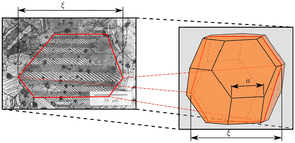
The left hand side of Figure 3 exhibits a micrograph of a BT grain. On the right hand side a truncated octahedron, as a model of a three-dimensional grain, is illustrated. The volume of a truncated octahedron is given by (Mendelson, 1969; Weisstein, 2003)

$$V=8\sqrt{2}{a}^3,$$

(27)

Figure 3.

Micrograph of a BT grain taken from Arlt (1990b) and truncated octahedron as model of a three-dimensional grain (in the style of Pearce, 1978).

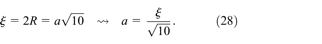
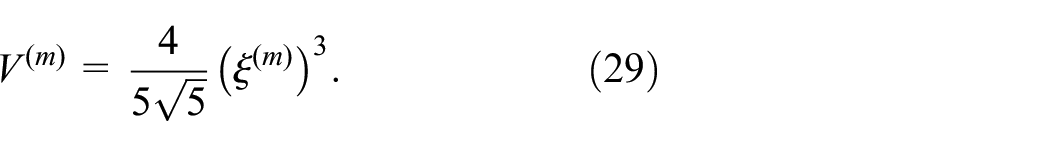
where $a$ represents the edge length according to Figure 3. The grain size $\xi$ being interpreted as the diameter $2R$ of the circumsphere, the following relation is obtained:

$$\xi =2R=a\sqrt{10}⇝a=\frac{\xi }{\sqrt{10}}.$$

(28)

It should be mentioned at this point that the volumes of the truncated octahedron and the circumsphere are not identical. The main characteristic of the circumsphere is that all vertices of the truncated octahedron are located on its surface. Inserting equation (28) into equation (27), the volume $V^{(m)}$ is finally given as a function of the grain size ${\xi }^{(m)}$ :

$$V^{(m)}=\frac{4}{5\sqrt{5}}{\left({\xi }^{(m)}\right)}^3.$$

(29)

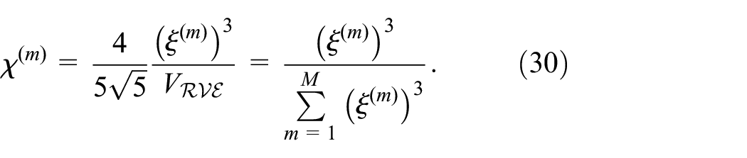
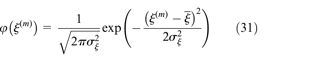
The volume fraction of a grain $m$ is thus obtained as

$${\chi }^{(m)}=\frac{4}{5\sqrt{5}}\frac{{\left({\xi }^{(m)}\right)}^3}{V_{\mathcal{R}\mathcal{V}\mathcal{E}}}=\frac{{\left({\xi }^{(m)}\right)}^3}{\sum _{m=1}^M{\left({\xi }^{(m)}\right)}^3}.$$

(30)

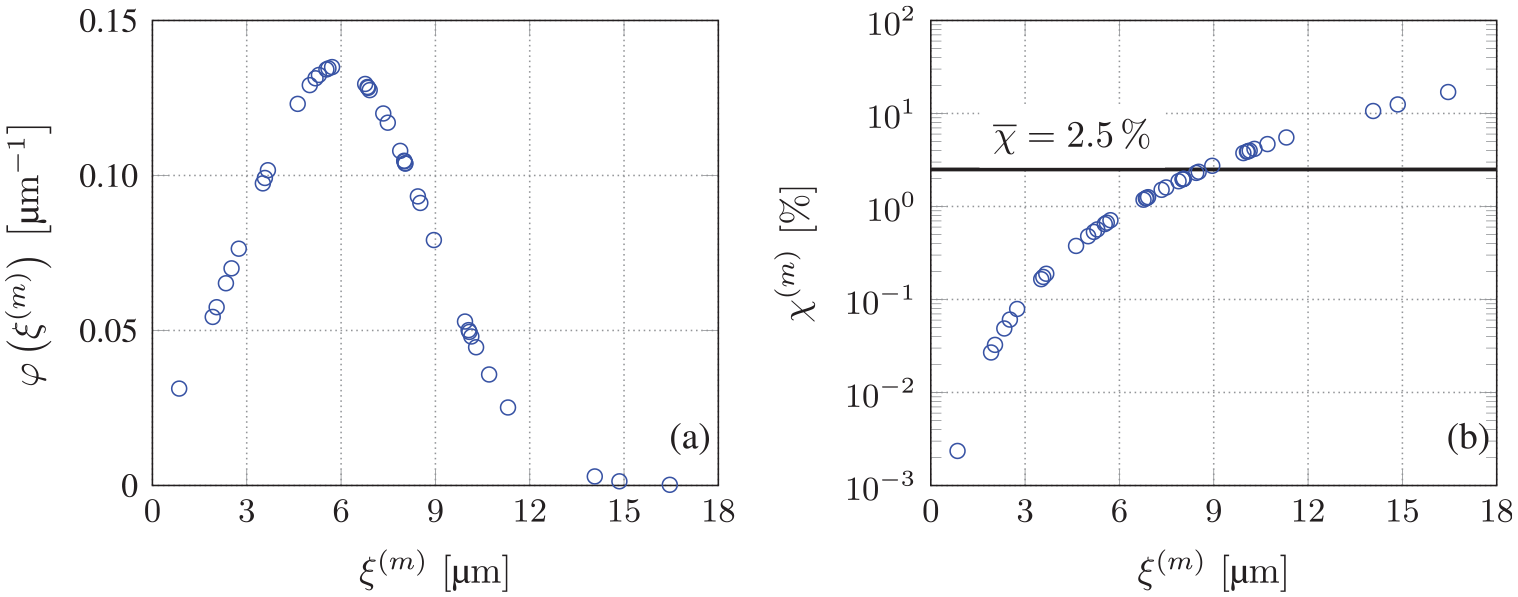
In the model, the grain sizes are assumed normally distributed. In Figure 4(a) and (b) the probability density function

$$\phi \left({\xi }^{(m)}\right)=\frac{1}{\sqrt{2\pi {\sigma }_{\xi }^2}}\exp (-\frac{{({\xi }^{(m)}-\overline{\xi })}^2}{2{\sigma }_{\xi }^2})$$

(31)

Figure 4.

(a) Probability density function $\phi ({\xi }^{(m)})$ and (b) volume fraction ${\chi }^{(m)}$ versus grain size ${\xi }^{(m)}$ of an $\mathcal{R}\mathcal{V}\mathcal{E}$ with $M=40$ grains, an average size $\overline{\xi }=5.9\mu \mathrm{m}$ and a standard deviation ${\sigma }_{\xi }=2.95\mu \mathrm{m}$ .

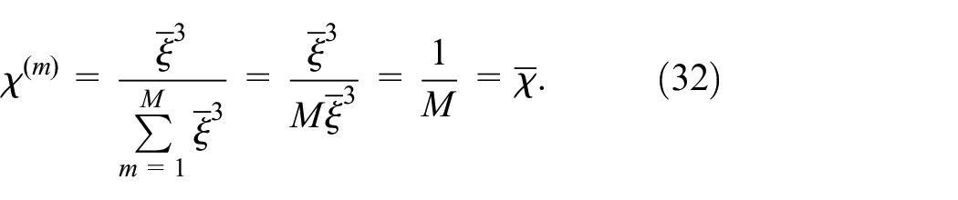
and the volume fraction ${\chi }^{(m)}$ according to equation (30), respectively, are plotted versus the grain size ${\xi }^{(m)}$ for an $\mathcal{R}\mathcal{V}\mathcal{E}$ with $M=40$ grains. As an example, an average grain size $\overline{\xi }=5.9\mu \mathrm{m}$ and a standard deviation ${\sigma }_{\xi }=2.95\mu \mathrm{m}$ are chosen. Figure 4(a) reveals the well known Gaussian distribution, where around $68\%$ of the grain sizes are located in a range of $\pm {\sigma }_{\xi }$ with respect to the averaged size $\overline{\xi }$ . In case of constant grain sizes, that is ${\xi }^{(m)}=\overline{\xi }$ , equation (30) yields

$${\chi }^{(m)}=\frac{{\overline{\xi }}^3}{\sum _{m=1}^M{\overline{\xi }}^3}=\frac{{\overline{\xi }}^3}{M{\overline{\xi }}^3}=\frac{1}{M}=\overline{\chi }.$$

(32)

From equations (30) and (32) it is obvious that the volume fraction ${\chi }^{(m)}$ does not depend on the volume of the $\mathcal{R}\mathcal{V}\mathcal{E}$ for a given number of grains $M$ , which uniquely determines the volume fractions in the case of uniform grains. For an $\mathcal{R}\mathcal{V}\mathcal{E}$ with $40$ grains $\overline{\chi }=2.5\%$ is obtained, which is indicated in Figure 4(b). Since the grain size is Gaussian distributed, around $68\%$ of the volume fractions are in a range of ${10}^{-1}\%<{\chi }^{(m)}<3\%$ , whereas for the whole $\mathcal{R}\mathcal{V}\mathcal{E}$ the range is ${10}^{-3}\%<{\chi }^{(m)}<20\%$ . The MiMP with a grain size $\xi \approx 16.5\mu \mathrm{m}$ and a corresponding volume fraction $\chi \approx 17\%$ can be mentioned as one example.

5. Parametric studies of ferroelectric $\mathcal{R}\mathcal{V}\mathcal{E}$ s

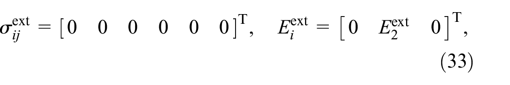
As an example for a ferroelectric material, BT is employed. The set of material parameters is found in the Appendix. For the numerical simulations a pure electric loading into the ${\mathit{e}}_2$ –direction, that is

$${\sigma }_{\mathrm{ij}}^{\mathrm{ext}}={\left[\begin{array}{cccccc}0\hfill & 0\hfill & 0\hfill & 0\hfill & 0\hfill & 0\hfill \end{array}\right]}^{\mathrm{T}},E_i^{\mathrm{ext}}={\left[\begin{array}{ccc}0\hfill & E_2^{\mathrm{ext}}\hfill & 0\hfill \end{array}\right]}^{\mathrm{T}},$$

(33)

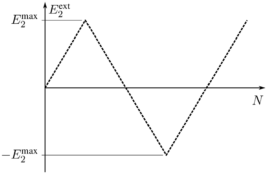
is considered. The applied electric load is realized by a trilinear function, where $E_2^{\max }=\pm 2·{10}^6\mathrm{V}{\mathrm{m}}^{-1}$ , see Figure 5. The constitutive framework has been implemented in a MATLAB code and calculations haven been performed on a MacBook Pro (2018) with a 2.7 GHz Quad-Core Intel i7 and 16 GB memory. Goals of this section are primarily to investigate the influences of different microscopic parameters on macroscopic quantities and a comparison with the available range of experimental findings.

Figure 5.

One cycle of a pure electric loading.

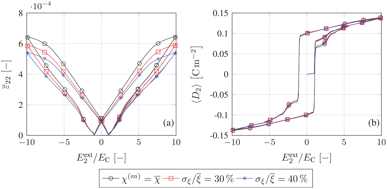
Before keeping the focus on characteristic magnitudes such as remanent or maximum values for quantitative investigations, Figure 6 shows hysteresis loops of strain and electric displacement taken from the first two load cycles. $M=40$ grains are employed in the $\mathcal{R}\mathcal{V}\mathcal{E}$ with the same arbitrary initial domain orientations as a basis for all three calculations. Whereas the butterfly loop, Figure 6(a), exhibits a distinct influence of statistical grain size distribution, represented by relative standard deviations of 30% and 40%, the electric displacement, Figure 6(b), is scarcely affected by non-uniform grain sizes. This effect can be explained by the dominant $180°$ domain wall motion, which is, with regard to equation (8), purely electrically driven and occurs instantaneously at $\pm E_{\mathrm{C}}$ . Due to the generalized VOIGT–approximation, s. equation (18), the electric field $E_i$ is assumed homogeneous in the $\mathcal{R}\mathcal{V}\mathcal{E}$ and is prescribed, that is, ${\overline{E}}_i=E_i^{\mathrm{ext}}$ . Therefore, $180°$ domain wall motion is independent of the relative standard deviation.

Figure 6.

(a) Butterfly and (b) dielectric hystereses of first two electric load cycles according to Figure 5 for uniform and Gaussian distributed grain size.

5.1. Magnitudes of grains and lower limits of domain volume fractions

In this subsection the influence of the number of grains (MiMPs) $M$ and the lower limit of the volume fractions ${\nu }_{\min }$ on remanent strain and polarization as well as maximum strain and computing time are investigated assuming uniform grain size. For this purpose, $\mathcal{R}\mathcal{V}\mathcal{E}$ s with 20, 30, 40, 50, 75, 100, and 200 grains are considered. Ten calculations with arbitrary initial domain orientations were performed in each case, requiring 70 numerical calculations in total. It has to be kept in mind that since absolute grain sizes are not relevant in the model, the parameter $M$ does not allow conclusions to be drawn about the size of the $\mathcal{R}\mathcal{V}\mathcal{E}$ . The “representative” aspect of the $\mathcal{R}\mathcal{V}\mathcal{E}$ is rather given by the number of arbitrary grain orientations increasing with the parameter $M$ .

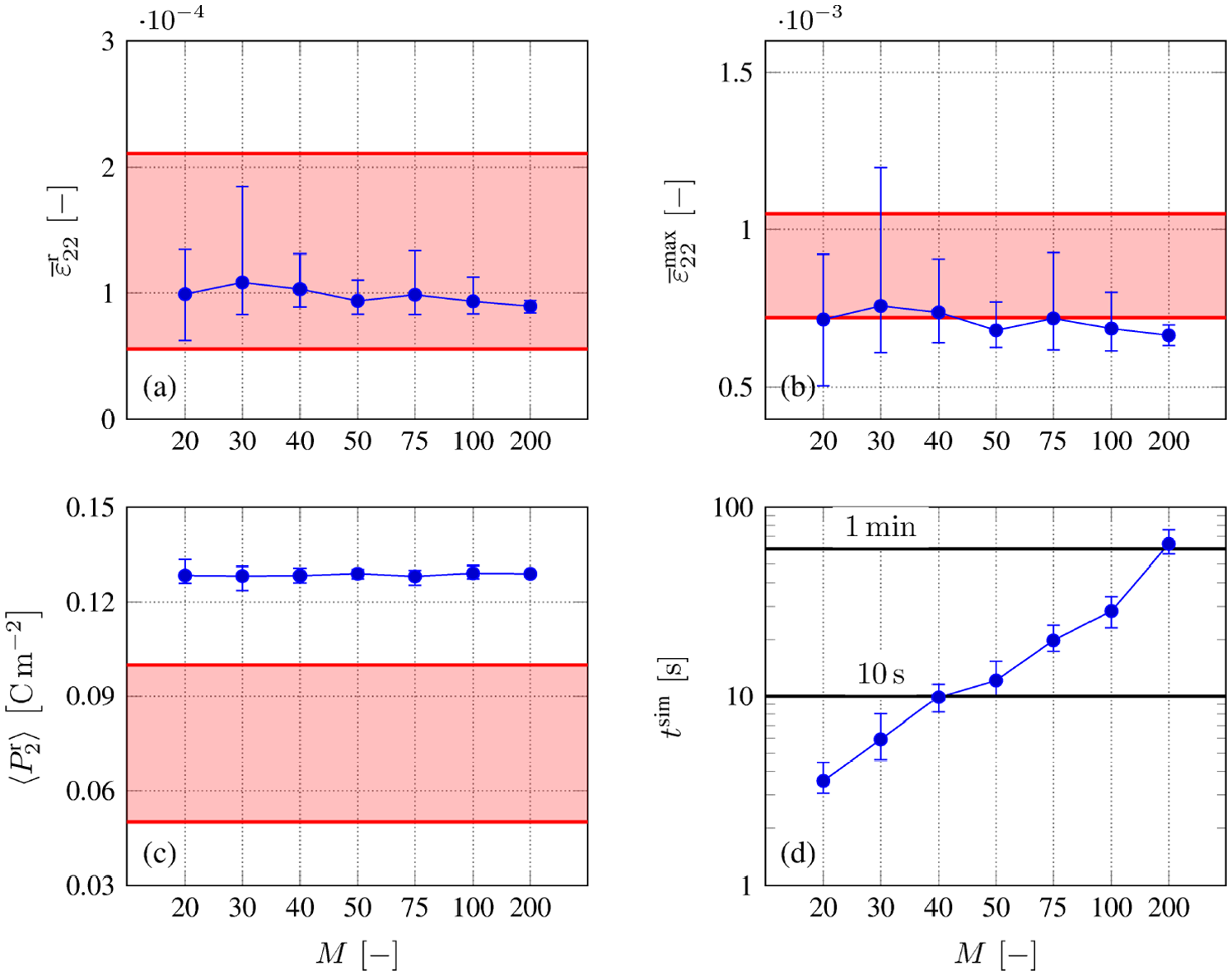
In Figure 7 error bars of the macroscopic remanent strain ${\overline{\epsilon }}_{22}^{\mathrm{r}}$ , maximum strain ${\overline{\epsilon }}_{22}^{\max }$ , remanent polarization $〈P_2^{\mathrm{r}}〉$ , and the computing time $t^{\mathrm{sim}}$ are plotted versus the number of grains $M$ . At this point ${\nu }_{\min }=0$ has been chosen for all calculations. Error bars depict the minimum, maximum, and mean values for each quantity. The red filled areas in Figure 7(a) to (c) represent the range of experimental data, taken from Enderlein (2007), Förderreuther (2003), and Wang and Li (2020). Having a look at the results of the remanent strain in Figure 7(a) the simulations are in a good accordance with experimental results independent of the number of MiMPs. Here, the mean values as well as the minima and maxima are within the area of experimental findings. For the maximum strain, see Figure 7(b), the mean values of the numerical simulations are located at the lower limit of experimental results. For 50, 100, and 200 MiMPs, the mean values are even slightly below the experimental range. Concerning the variances, two issues should be highlighted: an increasing number of MiMPs is basically attended by a decrease of the variance and the scattering of the maximum strain is larger than of the remanent strain. Both effects can be explained by the arbitrary orientations of MiMPs. The influence of a specific orientation in an $\mathcal{R}\mathcal{V}\mathcal{E}$ with 20 or 30 MiMPs is much larger than in an $\mathcal{R}\mathcal{V}\mathcal{E}$ with 100 or 200 MiMPs, since the strain ${\overline{\epsilon }}_{\mathrm{kl}}$ is an average quantity, see equation (23).

Figure 7.

(a) Macroscopic remanent strain ${\overline{\epsilon }}_{22}^{\mathrm{r}}$ , (b) maximum strain ${\overline{\epsilon }}_{22}^{\max }$ , (c) remanent polarization, $〈P_2^{\mathrm{r}}〉$ and (d) computing time $t^{\mathrm{sim}}$ versus number of grains $M$ . Red areas indicate the ranges of experimental data (Enderlein, 2007; Förderreuther, 2003; Wang and Li, 2020).

The number of MiMPs does not have a significant influence on the remanent polarization, Figure 7(c). In comparison to experimental results, however, the latter is larger, exceeding the upper value of the experimental range by about 25%. Since ${\nu }_{\min }=0$ and interactions between domains of a grain are not considered at this point, domains vanish in favor of others, finally overestimating predominantly the polarization. Figure 7(d) presents the effect of the number of MiMPs on the computing time $t^{\mathrm{sim}}$ . The semilogarithmic scale indicates the nonlinear relation between $M$ and $t^{\mathrm{sim}}$ . The simulation of one load cycle based on an $\mathcal{R}\mathcal{V}\mathcal{E}$ with 20 MiMPs takes about 3.5 s, whereas a simulation with 200 MiMPs takes about 1 min.

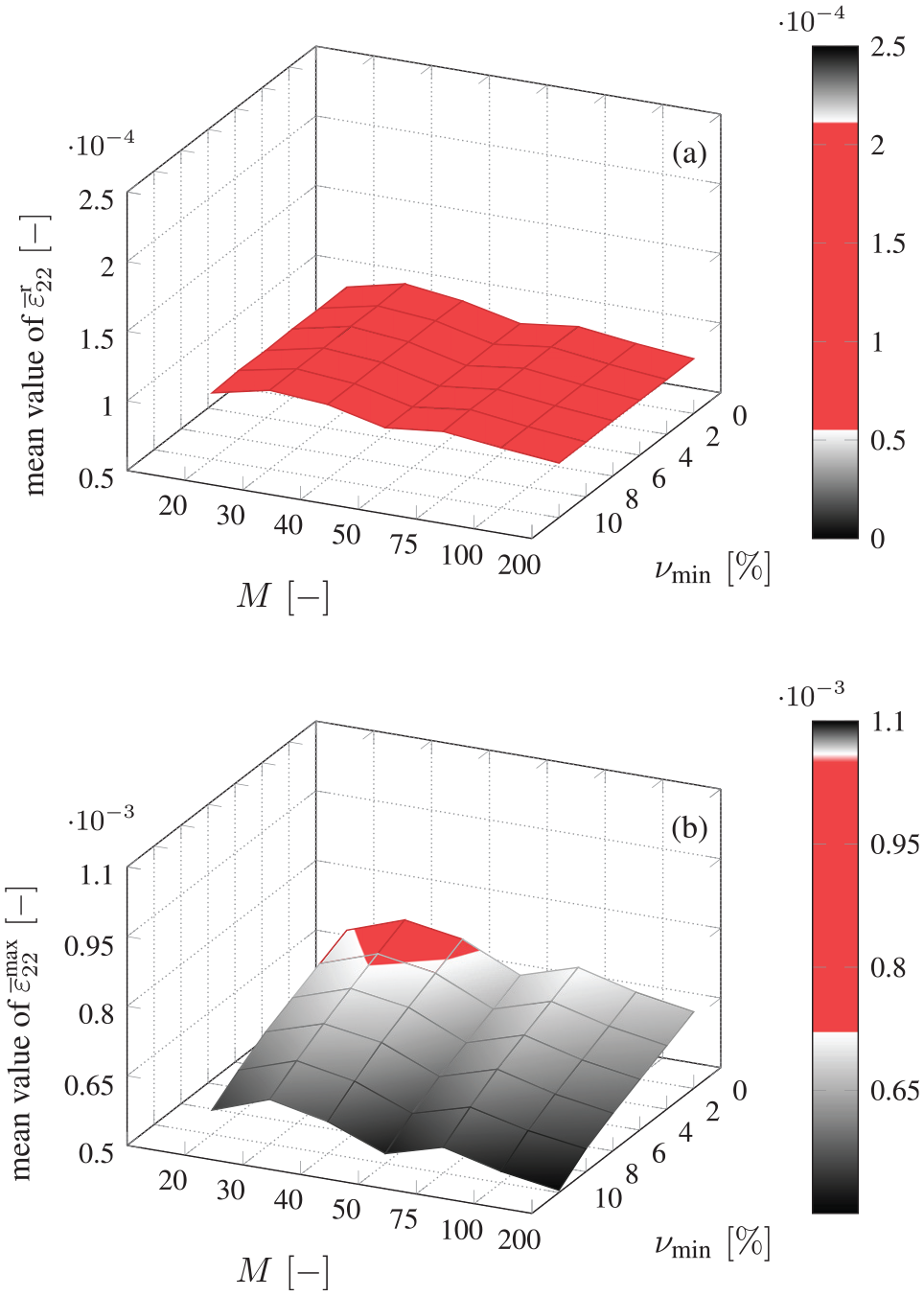
In Figures 8 and 9 the effect of a lower limit of domain volume fractions ${\nu }_{\min }$ is investigated. For each simulation discussed in Figure 7, five more with ${\nu }_{\min }$  = 2%, 4%, 6%, 8%, and 10% are considered. Requiring a total of 420 simulations, only the mean values are presented. Figure 8(a) shows the remanent strain ${\overline{\epsilon }}_{22}^{\mathrm{r}}$ , whereas Figure 8(b) exhibits the maximum strain ${\overline{\epsilon }}_{22}^{\max }$ versus the number of MiMPs and ${\nu }_{\min }$ . Values within the red colored areas match the range of experimental data outlined above. The impact of ${\nu }_{\min }$ on the remanent strain ${\overline{\epsilon }}_{22}^{\mathrm{r}}$ is negligible, see Figure 8(a). A significant influence of ${\nu }_{\min }$ , however, is observed at the maximum strain ${\overline{\epsilon }}_{22}^{\max }$ , see Figure 8(b). An increasing ${\nu }_{\min }$ reducing the amount of domain wall motion, a decrease of the maximum strain is one consequence. A ${\nu }_{\min }>>0$ thus underestimates the maximum strain and should be excluded.

Figure 8.

Mean values of (a) macroscopic remanent strain ${\overline{\epsilon }}_{22}^{\mathrm{r}}$ and (b) maximum strain ${\overline{\epsilon }}_{22}^{\max }$ taken from 10 simulations versus number of grains $M$ and the lower limit of the domain volume fractions ${\nu }_{\min }$ . Red areas match the scope of experimental data (Enderlein, 2007; Förderreuther, 2003; Wang and Li, 2020).

Figure 9.

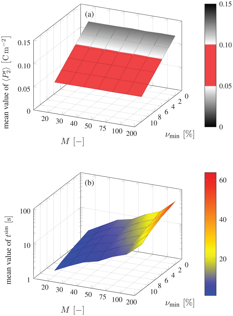
Mean values of (a) macroscopic remanent polarization $〈P_2^{\mathrm{r}}〉$ and (b) computing time $t^{\mathrm{sim}}$ taken from 10 simulations versus number of grains $M$ and the lower limit of the domain volume fractions ${\nu }_{\min }$ . Red area in (a) matches the scope of experimental data (Enderlein, 2007; Förderreuther, 2003; Wang and Li, 2020).

Figure 9(a) and (b) illustrates the remanent polarization $〈P_2^{\mathrm{r}}〉$ and the computing time $t^{\mathrm{sim}}$ , respectively, versus the number of MiMPs and ${\nu }_{\min }$ . As expected an increasing ${\nu }_{\min }$ leads to a decreasing remanent polarization and for ${\nu }_{\min }>2\%$ it is in a good accordance with the experimental data. Compared to the remanent strain of Figure 8(a), ${\nu }_{\min }$ has a significant influence on the remanent polarization. This effect is caused by $180°$ switching processes, having no impact on the irreversible strain. Reducing the magnitude of domain switching, an increasing ${\nu }_{\min }$ leads to a decreasing computing time, see Figure 9(b). For $M=40$ and ${\nu }_{\min }=4\%$ , for example, a time saving of 30% is achieved. On the basis of the above investigations, the parameters $M$ and ${\nu }_{\min }$ can now be chosen reasonably with regard to experimental results and computational costs. In this context, $M=40$ and ${\nu }_{\min }=4\%$ seem to be a good choice for all following investigations, whereupon ${\overline{\epsilon }}_{22}^{\mathrm{r}}$ and $〈P_2^{\mathrm{r}}〉$ are in a very good accordance with experimental data, while the mean value of ${\overline{\epsilon }}_{22}^{\max }=6.8073·{10}^{-4}$ is just slightly below the experimental range. The corresponding average computing time is approximately 7 s per load cycle.

5.2. Stochastic distribution of grain size

In this subsection, the influence of normally distributed grain sizes on the remanent strain and polarization as well as maximum strain and computing time are investigated. Based on the study outlined in the previous subsection, an $\mathcal{R}\mathcal{V}\mathcal{E}$ with $M=40$ MiMPs and ${\nu }_{\min }=4\%$ will be considered in the following. Concerning a reasonable range for the standard deviation of ceramic grain structures, relative values ranging from 4.25%, see Chinn (1994), to 35%, see Manosso et al. (2010), are found in the literature, where the standard deviation is normalized with respect to the average grain size. For the numerical simulations an average grain size of $\overline{\xi }=5.9\mu \mathrm{m}$ is considered, representing a reasonable value for fine-grained BT. Based on the literature, standard deviations between ${\sigma }_{\xi }=0.295\mu \mathrm{m}$ and ${\sigma }_{\xi }=2.36\mu \mathrm{m}$ should be an appropriate range. However, for the sake of a convergence study, standard deviations from $5.9·{10}^{-4}\mu \mathrm{m}$ to $2.95\mu \mathrm{m}$ are considered, the former representing the limiting case of a uniform grain size. Again, ten different $\mathcal{R}\mathcal{V}\mathcal{E}$ s are taken into account for each value of ${\sigma }_{\xi }$ , whereat the same sets of domain orientations as used in the previous subsection were chosen.

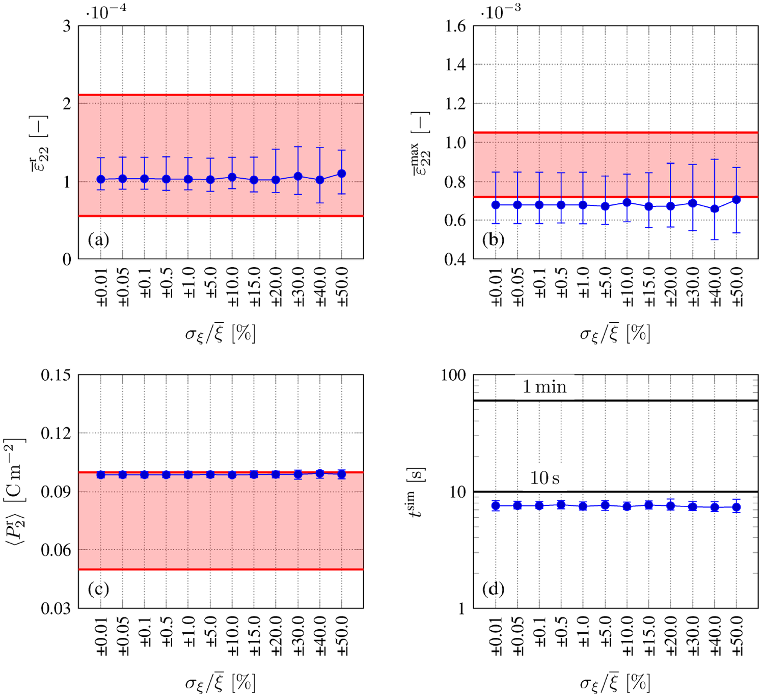
In Figure 10 ${\overline{\epsilon }}_{22}^{\mathrm{r}}$ , ${\overline{\epsilon }}_{22}^{\max }$ , $〈P_2^{\mathrm{r}}〉$ and $t^{\mathrm{sim}}$ are plotted versus the normalized standard deviation ranging from 0.01% to 50%. According to Figure 10(a) and (b), only standard deviations above 0.885  $\mu$ m, that is, ${\sigma }_{\xi }/\overline{\xi }\ge 15\%$ , have a noticeable impact on the remanent and maximum strains in terms of the interval widths. The grain size distribution further has no essential influence on the remanent polarization, see Figure 10(c), where the intervals are small anyway. For the computing time $t^{\mathrm{sim}}$ , Figure 10(d), no substantial impact is observed either.

Figure 10.

(a) Macroscopic remanent strain ${\overline{\epsilon }}_{22}^{\mathrm{r}}$ , (b) maximum strain ${\overline{\epsilon }}_{22}^{\max }$ , (c) remanent polarization, $〈P_2^{\mathrm{r}}〉$ and (d) computing time $t^{\mathrm{sim}}$ versus normalized standard deviation for an $\mathcal{R}\mathcal{V}\mathcal{E}$ with $M=40$ grains and ${\nu }_{\min }=4\%$ . Red areas indicate the range of experimental data (Enderlein, 2007; Förderreuther, 2003; Wang and Li, 2020).

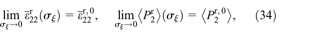
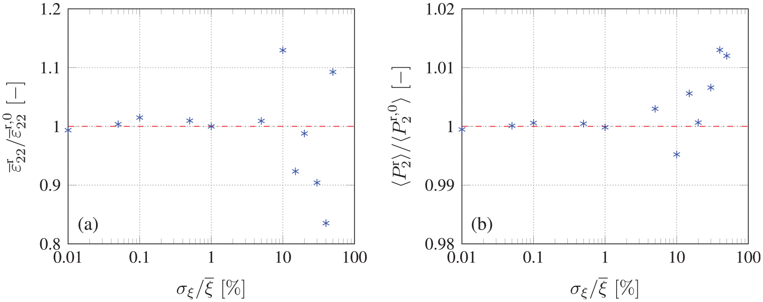
Figure 11 presents the results of a convergence study. Here, remanent strain and polarization, normalized with respect to the values of the same $\mathcal{R}\mathcal{V}\mathcal{E}$ with identical initial domain orientations, however, a uniform grain size ${\overline{\epsilon }}^{\mathrm{r},0},〈P^{\mathrm{r},0}〉$ , are plotted versus the normalized standard deviation in a range from 0.01% to 50%. All asterisks here and in the following represent the same set of grain orientations. The limiting values of ${\overline{\epsilon }}_{22}^{\mathrm{r}}$ and $〈P_2^r〉$ for ${\sigma }_{\xi }\to 0$ , as expected, correspond to the magnitudes of uniform grain size, that is,

$$\underset{{\sigma }_{\xi }\to 0}{lim}{\overline{\epsilon }}_{22}^{\mathrm{r}}\left({\sigma }_{\xi }\right)={\overline{\epsilon }}_{22}^{\mathrm{r},0},\underset{{\sigma }_{\xi }\to 0}{lim}〈P_2^{\mathrm{r}}〉\left({\sigma }_{\xi }\right)=〈P_2^{\mathrm{r},0}〉,$$

(34)

Figure 11.

(a) Remanent strain and (b) polarization normalized with respect to the values of a uniform grain size versus normalized standard deviation for $M=40$ grains and ${\nu }_{\min }=4\%$ .

which is confirmed by Figure 11 and emphasizes the consistency of the model in this respect. Figure 11 also illustrates the sudden increase of scattering of strain and polarization for relative standard deviations above 10%.

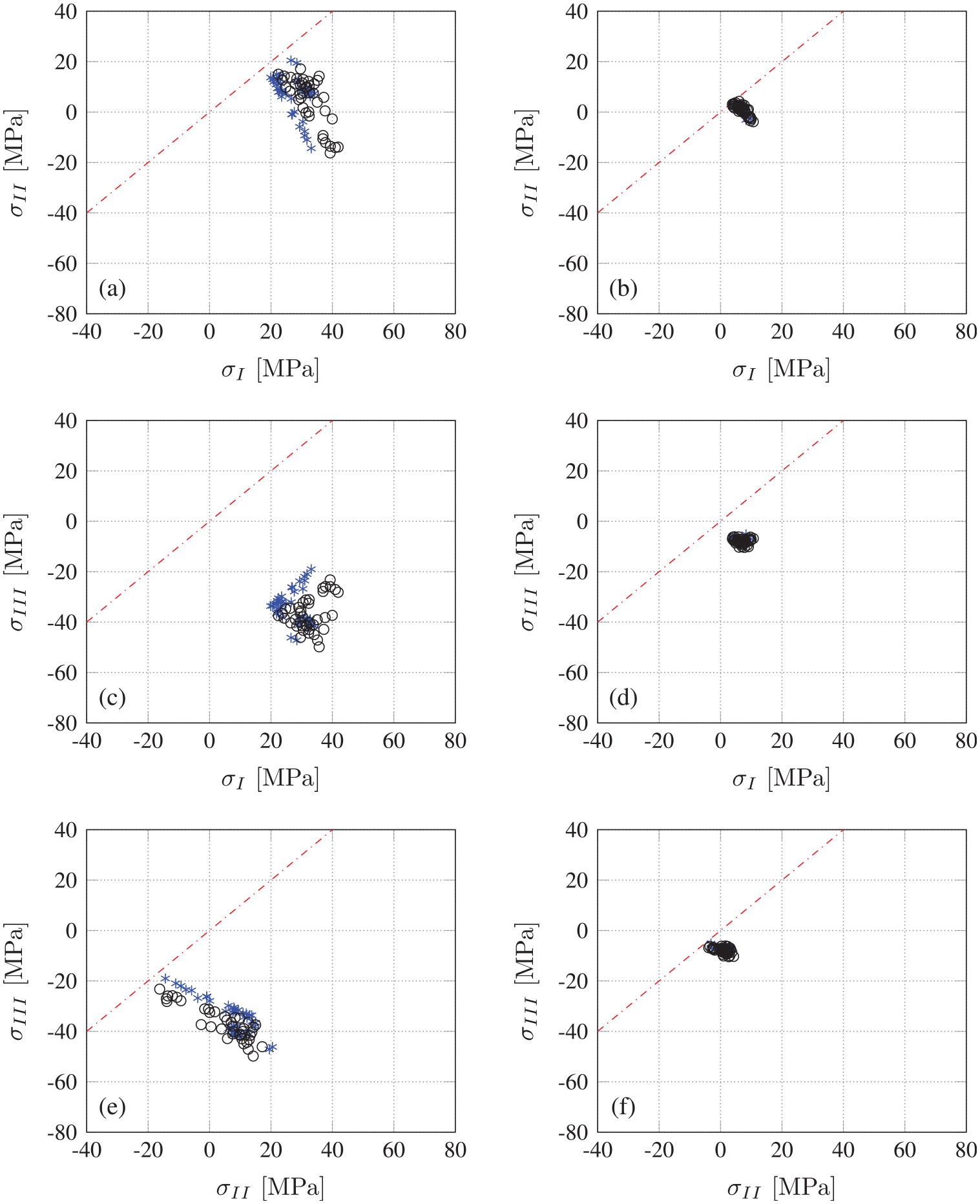
Figure 12 finally presents principal residual stresses at $E_2=E_2^{\max }$ and $E_2=0$ after unloading. The black circles represent the results of uniform grain size, while the blue asterisks denote those of grain size distribution, where ${\sigma }_{\xi }=2.36\mu \mathrm{m}$ and ${\sigma }_{\xi }/\overline{\xi }=40\%$ , respectively. Since ${\sigma }_I>{\sigma }_{\mathrm{II}}>{\sigma }_{\mathrm{III}}$ by convention, the stresses are restricted to the area below the red dash–dotted lines. Independent of the applied electric field, the black circles are concentrated to restricted areas in the space of principal stresses. This issue has already been observed in Lange and Ricoeur (2015), where the principal stresses of the CM were compared to those from FE simulations based on the same micro-mechanical model of domain switching. It should be noted, that in Lange and Ricoeur (2015) a 2D approach was considered, while 3D is adopted in this work, however, not showing a considerable impact on this aspect. For $E_2=0$ , Figure 12(b), (d), and (f), there are no significant differences between $\mathcal{R}\mathcal{V}\mathcal{E}$ s with distributed or uniform grain sizes, whereas at $E_2=E_2^{\max }$ , Figure 12(a), (c), and (e), an influence is observed, although all values are basically arranged in the same areas.

Figure 12.

Principal residual stresses at $E_2=E_2^{\max }$ ((a), (c) and (e)) and $E_2=0$ ((b), (d) and (f)) after unloading of an $\mathcal{R}\mathcal{V}\mathcal{E}$ with $M=40$ MiMPs and ${\nu }_{\min }=4\%$ for a uniform grain size (black circles) and a standard deviation of ${\sigma }_{\xi }=2.36\mu \mathrm{m}$ (blue asterisks - ${\sigma }_{\xi }/\overline{\xi }=40\%$ ).

6. Conclusion

A basically approved microphysically motivated scale-bridging polycrystalline constitutive approach has been augmented in two different aspects. Domains are not allowed to vanish in favor of others by introducing constraints to domain volume fractions, and grain sizes are non-uniform, following a Gaussian distribution. Barium titanate, as extensively investigated ferroelectric with unique chemical composition, has been chosen for the sake of experimental validation. Data have been compiled in this regard from various references to compare key quantities of hysteresis loops to results of simulations. Arbitrary orientations of grains in an $\mathcal{R}\mathcal{V}\mathcal{E}$ require a statistical analysis, finally providing a very good agreement with experiments, adapting not more than two model parameters, that is, number of grains in an $\mathcal{R}\mathcal{V}\mathcal{E}$ and lower limit of domain volume fractions. The grain size distribution turns out to have a noticeable impact for relative standard deviations above 10%–15%, leading to an increasing scatter of predominantly strain, whereas polarization and residual stresses are scarcely influenced in their magnitudes. The computing time of one electric load cycle on a MacBook Pro is just a few seconds, emphasizing the efficiency of the modeling approach.