
Abstract
Magnetorheological fluids involve multi-physics phenomena which are manifested by interactions between structural mechanics, electromagnetism and rheological fluid flow. In comparison with analytical models, numerical models employed for magnetorheological fluid applications are thought to be more advantageous, as they can predict more phenomena, more parameters of design, and involve fewer model assumptions. On that basis, the state-of-the-art numerical methods that investigate the multi-physics behaviour of magnetorheological fluids in different applications are reviewed in this article. Theories, characteristics, limitations and considerations employed in numerical models are discussed. Modelling of magnetic field has been found to be rather an uncomplicated affair in comparison to modelling of fluid flow field which is rather complicated. This is because, the former involves essentially one phenomenon/mechanism, whereas the latter involves a plethora of phenomena/mechanisms such as laminar versus turbulent rheological flow, incompressible versus compressible flow, and single- versus two-phase flow. Moreover, some models are shown to be still incapable of predicting the rheological nonlinear behaviour of magnetorheological fluids although they can predict the dynamic characteristics of the system.
Keywords
1. Introduction
In this introductory section, a survey on the history, current applications, advantages and disadvantages of magnetorheological (MR) fluids is presented. The survey shows the growing interest in the employment of MR fluids in different applications in the last 20 years. This growing interest heightens the need for better prediction of flow characteristics. Then, the characteristics of MR fluid flow and flow modes manifested in different MR devices are presented. Finally, the contents of the later sections of this article, which focuses on reviewing numerical methods applied to MR fluids in different applications, are outlined.
1.1. History and current applications of MR fluids
Generally, smart fluids can detect an external stimulus and therefore, change their characteristics accordingly in a non-traditional manner. MR fluids are semi-active smart fluids whose employment in different engineering devices is continuously growing since 1990s (Spaggiari et al., 2019; Yuan et al., 2019). MR fluids, which were first invented by Jacob Rabinow in 1947, are suspensions of ferromagnetic particles in a suitable carrier fluid (Rabinow, 1947; Wang and Liao, 2011). The smart behaviour of MR fluids is indicated by the controllable increase of their apparent viscosity under the effect of an external tunable magnetic field. Viscosity increase is manifested due to queue of ferromagnetic particles in rigid networks of chains, which converts the fluid nature into a semi-solid state with a considerable yield stress (Gołdasz and Sapiński, 2015b). Therefore, MR fluids exhibit elastic, plastic and viscous flow characteristics in the activated mode. This flow behaviour can be termed as ‘viscoelastic-plastic’ flow (Wang and Liao, 2011).
The remotely controllable characteristics of MR fluids attract continuous research on the employment of MR fluids in different applications (Ahamed et al., 2018). MR dampers are the most well-known MR fluid devices that are currently found in some luxury cars and ambulances (Bai et al., 2013, 2015; Boada et al., 2011; Chae and Choi, 2015; Gurubasavaraju et al., 2018a). Moreover, MR dampers are also being researched for different applications other than automotive. These applications may include, but not limited to: cushions in civil buildings and bridges (Ding et al., 2013; Wu, 2010), railway suspension (Kim et al., 2016a), tracked vehicles (Ata and Oyadiji, 2014), prosthesis (Case et al., 2014; Qiang et al., 2017), dampers for washing machine rotary parts (Ulasyar and Lazoglu, 2018), gun recoil dampers (Ahmadian and Norris, 2008; Hu et al., 2012), helicopter cockpit seats (Hiemenz et al., 2008; Singh and Wereley, 2015), and aircraft landing gears (Han et al., 2019). In the past 10 years, MR dampers were researched to incorporate self-powering, self-controlling and energy harvesting characteristics in order to operate in the absence of a power source (Chen and Liao, 2012; Sapiński, 2011; Wang and Wang, 2009; Wang et al., 2010). Also, research on MR dampers with variable stiffness and damping force has attracted more interest recently (Deng et al., 2019; Huang et al., 2019).
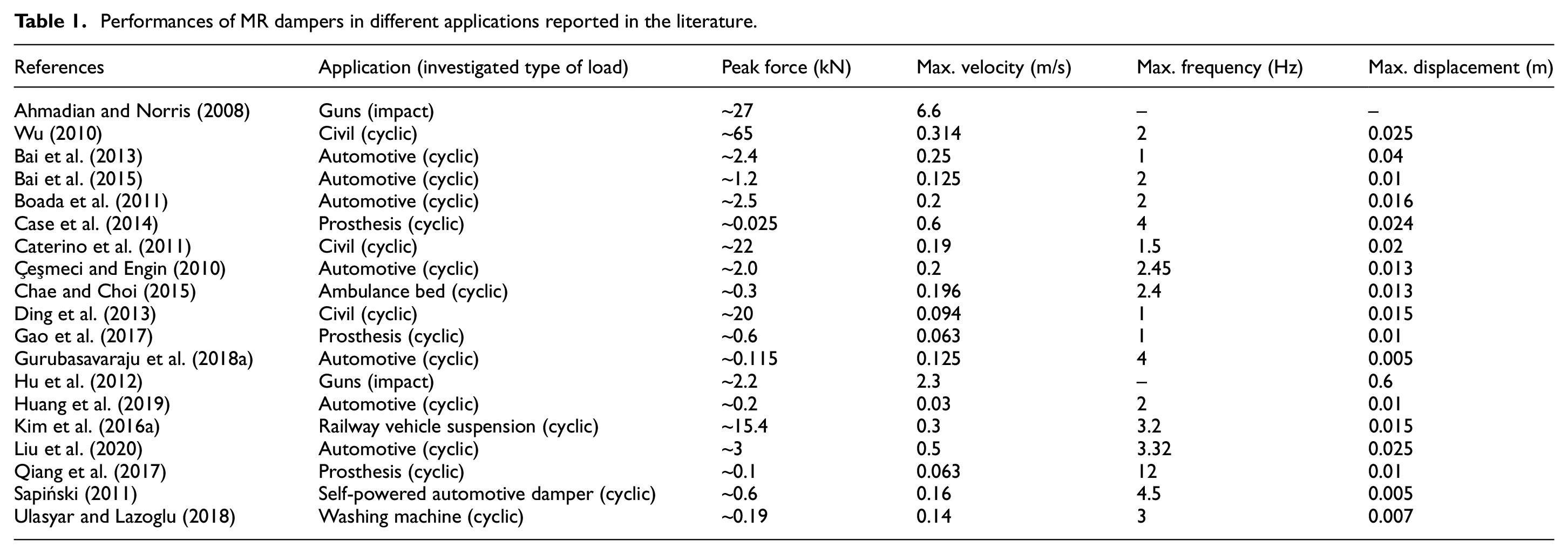
Table 1 shows some numeric values that report the performance of MR dampers employed in different applications that are researched in the literature. It can be seen that MR dampers are suitable for a wide range of force, velocity and displacement scales. The highest force scales are applied within military, railway and civil engineering applications, whereas the force scales are relatively smaller in automotive applications and are significantly lower in prosthetics. Most MR dampers operate at low values of motion frequency and amplitude except for gun recoil dampers, in which the velocity and motion amplitudes are extremely high. A commercial piece of weapon which employs an MR damper has not been reported yet. It should be noted that the performance of MR dampers at such higher scales of forces and velocities is quite different. That is due to the effects of inertia, turbulence, viscoelasticity and fluid compressibility, which affect the performance of the damper greatly (Ahmadian and Norris, 2008; Kim et al., 2015; Li and Wang, 2012; Singh et al., 2014).
Performances of MR dampers in different applications reported in the literature.
Moreover, MR fluids are researched to replace conventional fluids in commercial applications other than MR dampers. The performances of these applications are found to improve significantly due to the rapid, reversible and controllable characteristics of MR fluids (Wang and Liao, 2011). Examples of these applications are journal bearings (Bompos and Nikolakopoulos, 2011), hydraulic valves (Bullough et al., 2008; Nguyen et al., 2008), micro-pumps (Liang et al., 2018), smart clutches (Ellam et al., 2006; Zhang et al., 2019), rotary MR dampers (Deng et al., 2019; Wang et al., 2019), robotics (Hartzell et al., 2019; Hwang et al., 2019), energy harvesters (Deng and Dapino, 2015; O’Donoghue et al., 2016), rheometers (Allebrandi et al., 2020), human prosthesis (El Wahed and Wang, 2019), engines mounts (Do and Choi, 2015), and hybrid body armours (Son and Fahrenthold, 2012). So far, there have been fewer studies on the employment of MR fluids in these applications compared to research efforts on linear MR dampers (Galindo-Rosales, 2016).
Table 2 shows some data from different research papers that investigate the employment of MR fluids in applications other than MR dampers. The methods applied, parameters of interest, and main findings of each research paper are summarised. It can be deduced from the table that the employment of MR fluids in these applications was proved to be effective in many devices. However, the methods applied for modelling and simulating the performances of these devices are diverse and may be quite complicated due to the highly nonlinear behaviour of MR fluids caused by their multi-physics nature. The models developed for MR dampers are thought to be achievable compared to those developed for other MR fluid devices. That is because, the common models developed for MR dampers depend on the representation of an MR damper as a nonlinear mechanical system composed of a set of springs and dashpots (Wang and Liao, 2011). These models can predict the kinetics of the damper, but they cannot predict the dynamic rheological behaviour of the MR fluid which may be essential to be modelled, but quite complicated, in some other MR fluid applications.
Research on employment of MR fluids in different applications other than MR dampers.
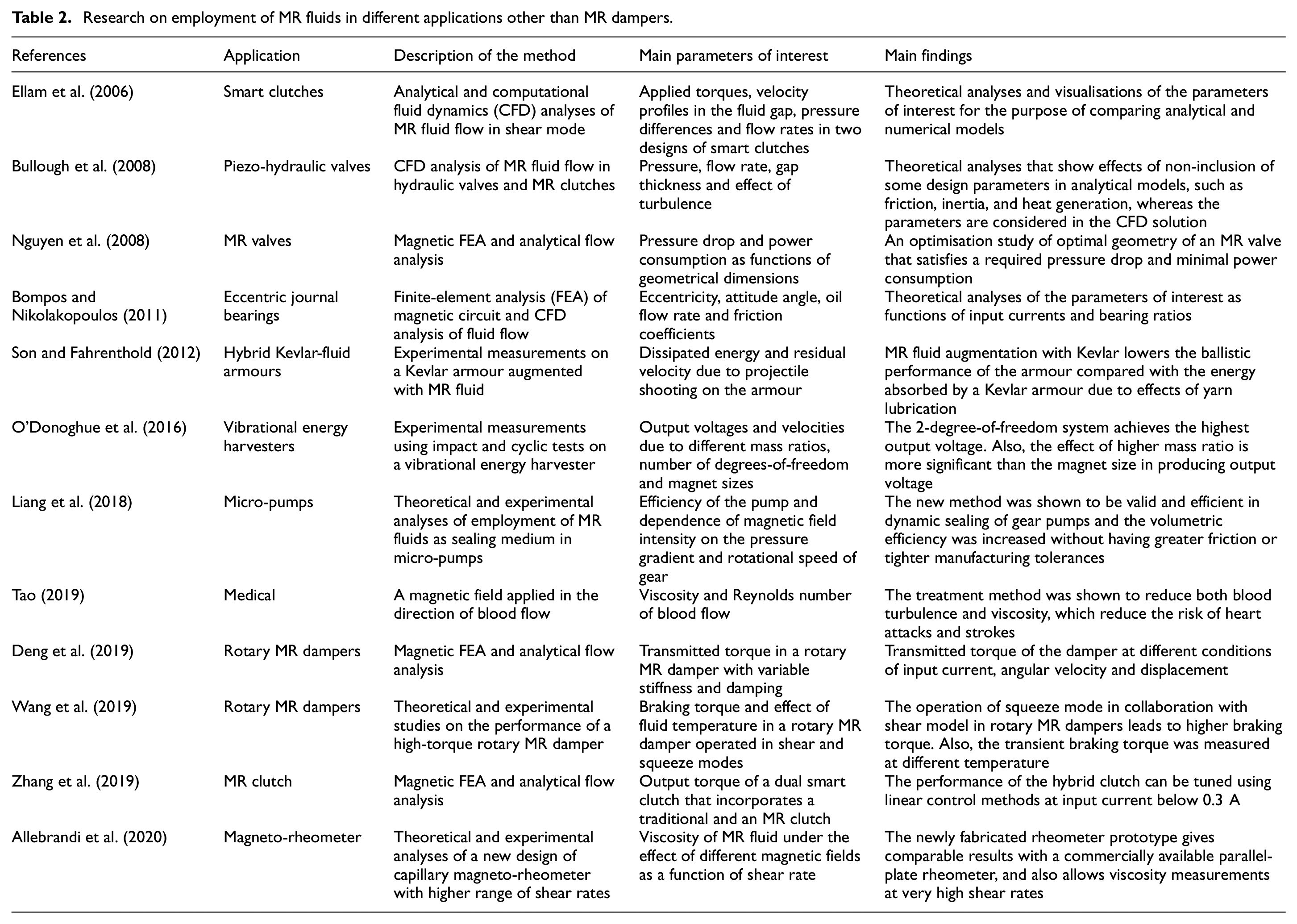
One of the latest discoveries of the applications of magnetic field in medical purposes has been recently presented by Tao (2019). Magnetic field has been employed to decrease blood viscosity and turbulence with the aim of reducing risks of heart attacks and strokes, as shown in Table 2. That is because blood is a paramagnetic fluid, as it contains haemoglobin, so it slightly attracts to magnetic fields. The new method has been proven to be effective. Magnetic field is applied externally in the same direction of blood flow. This causes blood viscosity to be anisotropic and also leads to suppress turbulence. Therefore, the load on heart to pump blood reduces. Blood flow is rather a complicated non-Newtonian flow in which the elastic properties of veins affect the flow characteristics (Ibrahim et al., 2017; Tazraei et al., 2015). The same principle was also shown to be employed to reduce viscosity and suppress turbulence in the flow of crude oil in oil pipelines (Du et al., 2018).
1.2. Advantages and disadvantages of MR fluids
As shown in the preceding section, the usage of MR fluids is shown to be advantageous in many applications. The advantageous performance of an MR fluid device is achieved when the fluid is operated within a proper automatic control circuit (Rossi et al., 2018). The optimally controlled magnetic field in an MR fluid system can conduce the requisite performance of the system. For instance:
An ideal curve of hydraulic resistance can be obtained by the employment of an MR gun recoil damper, as suggested by Hu et al. (2012). The idealised hydraulic resistance leads to reducing the overall force transmitted to gun systems, as shown schematically in Figure 1(a). This idealised force cannot be attained by the employment of a conventional fluid, even if a variable throttling area along the recoil stroke of the conventional recoil damper is implemented to control the hydraulic resistance.
Better vibration control is also reported as another advantage of the employment of control loop in MR dampers (Ata and Oyadiji, 2014; Hiemenz et al., 2008). For example, a better vibration control of an MR damper was achieved by Hiemenz et al. (2008), as shown in Figure 1(b). The better vibration control that can be indicated by the transmissibility curve (output acceleration divided by input acceleration of the piston) was achieved due to the employment of a semi-active Skyhook control algorithm that controls the excitation current of the damper. It can be seen that the transmissibility curve due to applying the Skyhook control algorithm is better than the counterparts obtained by applying either a constant or no magnetic field. Research on better performance of MR dampers due to the employment of control loops attracts more interests, as reported by Christie et al. (2019) and Liu et al. (2019). A rotary MR damper employed with the purpose of seismic vibration suppression was presented by Christie et al. (2019). The damper performance was tuned by a short-time Fourier transform (STFT) control algorithm. On the other hand, a proportional–integral–derivative (PID) controller was employed by Liu et al. (2019) to control the performance of a linear MR damper. The performances of MR dampers due to the employment of different types of controllers were investigated by Sun et al. (2019).
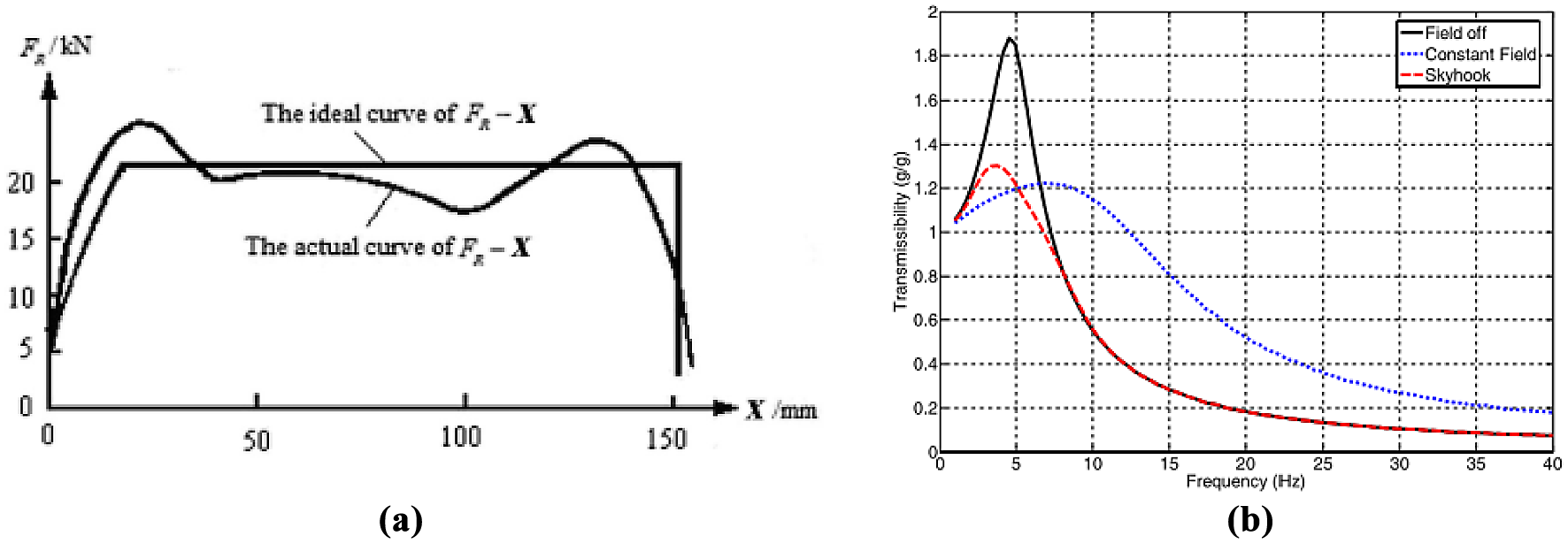
Idealised performance of MR dampers operated within automatic control loops: (a) theoretical force–displacement diagram of an MR gun recoil damper (Hu et al., 2012), and (b) theoretical transmissibility curve of an MR damper in off-, on-, and controllable modes using a semi-active skyhook control algorithm (Hiemenz et al., 2008).
On the other hand, it is thought to be the main disadvantage of MR fluids is the sedimentation of relatively denser ferromagnetic particles in carrier fluids. Sedimentation was first researched by Winslow (1953), and it is thought to be the main challenge to the employment of MR fluids in many applications since that date (Chooi, 2005). A typical MR fluid is composed of magnetic micro-sized particles, a carrier fluid and additives in the form of dispersants and surfactants whose main roles are to control particle sedimentation and secure easy mixing of the particles in the carrier fluid (Chooi, 2005). Controlling sedimentation motivated research on the longevity of stability of MR fluids in stored state. Various methods of controlling sedimentation were reviewed by Ashtiani et al. (2015). The study categorises these methods as follows: (1) coating the particles with a less-dense material relative to the fluid, (2) using nano-sized spherical or wired-shaped particles, (3) changing the carrier fluid type and the concentration of ferromagnetic particles, (4) using various types of surfactants and dispersants, and (5) using other unconventional methods, such as preserving MR fluids in the stored state in porous media, as suggested by Liu et al. (2011). That porous media evoke the fluid out under the effect of magnetic field. A ‘dry’ MR fluid that does not employ a carrier fluid was fabricated by Nakano et al. (2015). The ‘fluid’ was not only found to lack to the sedimentation problem but also the magnetic effect was found to be higher due to the higher content of iron powder. However, it is thought that more considerations regarding controllability and sealing of the fluid should be accounted for in the use of this kind of fluid.
Other disadvantages of MR fluids are reported in the literature, namely temperature rise of MR fluids which affects their viscosity and durability of MR fluids (Gołdasz and Sapiński, 2015b). Many parameters can be grouped under the term of durability, such as (1) safety of MR devices in passive mode, (2) need of a power source which may be a limitation in some devices, (3) the high cost of MR fluids in comparison with conventional fluids, (4) the compatibility of MR fluids in different devices, and (5) the in-use thickening (IUT) problem in which an MR fluid is transferred to a paste due to operation in the activated mode for a long time (Chooi, 2005). It is reported that the IUT problem was identified and overcome by Gołdasz and Sapiński (2015b). However, due to continuous development in production of MR fluids, it is thought that the IUT problem still needs to be researched, as found by Utami et al. (2018). In that paper, it was shown that the characteristics of a commercial MR fluid, produced by CK Material Laboratory in Korea, change considerably due to the IUT problem. In fact, there is quite limited research effort towards the durability of MR fluids in different applications, and very rare research papers that report a generalised failure theory of an MR device (Bigué et al., 2019; Gołdasz and Sapiński, 2015b).
1.3. Rheology of MR fluids
Rheology is derived from a Greek word that means ‘flow’, and it can be defined as the study of flow of liquids and soft solids (Gedik et al., 2012; Schowalter, 1978). The viscoelastic-plastic behaviour of MR fluids under shear load conditions can be illustrated as follows (Ashour and Rogers, 1996; Wang and Liao, 2011); the fluid behaves elastically in the pre-yield region
1.3.1. Models of viscoplastic flow
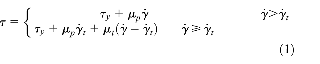
The most popular viscoplastic models used with MR fluids are the Bingham plastic and the Herschel–Bulkley models (Bingham, 1922; Herschel and Bulkley, 1926). Some other viscoplastic expressions were introduced by Casson (1959), Sisko (1958) and Robertson and Stiff (1976). The later models are commonly used to study viscoplastic fluids other than MR fluids, such as mud, slurries and blood flows (Imran et al., 2001; Kelessidis and Maglione, 2006; Kundu and Cohen, 2016). The constitutive equations of these models are shown in Table 3.
Typical rheological models for yielded fluids.
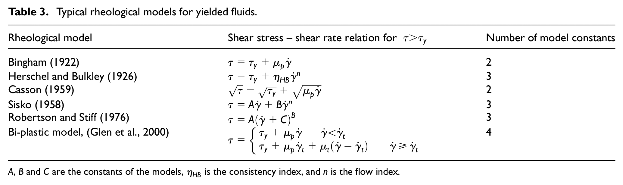
The number of constants of models presented in Table 3 indicates the degree of model complexity. Models with more constants were presented by Chooi and Oyadiji (2009). Nevertheless, defining the shear stress over a wide range of shear rates with a single equation may not be sufficient for the accurate prediction of shear-thinning behaviour. A bi-plastic equation was proposed by Glen et al. (2000). The shear stress is defined according to the following equation
where
1.3.2. Models of viscoelastic flow of MR fluids
Viscoelastic effects are usually neglected in most MR applications, as these effects are commonly reported to be minor compared to the effects of viscoplasticity (Gurubasavaraju et al., 2018a; Syrakos et al., 2016, 2018). It should be also noted that the constitutive equations of viscoelastic fluids are relatively difficult which may be another reason for neglecting viscoelastic effects (Syrakos et al., 2018). The viscoelastic behaviour is most importantly to be investigated when studying the deformation of some materials, such as polymers (Goktekin et al., 2004), elastomers (Yang et al., 2013), metals at very high temperatures (Saramito, 2016), and fluids with super high viscosity (Syrakos et al., 2018).
The Maxwell and the Kelvin–Voigt models are the most common models that study the deformations of viscoelastic materials. Both models represent a viscoelastic material as a combination between a purely viscous dashpot and a purely elastic spring (Wikipedia, 2004). The dashpot and the spring are connected in series in the Maxwell model, whereas they are connected in parallel in the Kelvin–Voigt model. The constitutive equations of both models can be written, respectively, as (Meyers and Chawla, 2008)

where
Later models of viscoelasticity that combine the effects of both of the Maxwell and the Kelvin–Voigt models were developed to allow more flexibility of the models. These models apply more springs and dashpots configured in series and parallel connections in their schematic representations. However, the models have more complicated equations and more parameters to be determined. Examples of these models are the standard linear solid (Zener) model, the Burgers model, the Biot model and the generalised Maxwell model (Biot, 1956; Butz and Stryk, 2002; Joseph, 1990; Meyers and Chawla, 2008).
1.4. Flow modes of MR fluids
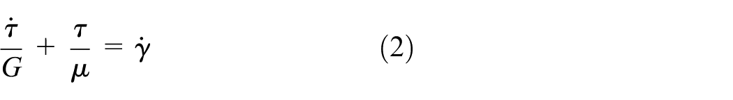
Depending on each MR fluid application, flow of MR fluids can be characterised into four modes, namely flow (valve) mode, shear mode, squeeze mode and pinch mode (Gołdasz and Sapiński, 2015b; Yu et al., 2016). The flow characteristics of each flow mode are shown schematically in Figure 2. The figure shows the direction of magnetic field and the one-dimensional (1D) velocity profile of fluid flow in each mode. In flow (valve) and pinch modes, Figure 2(a) and (d), the magnetic poles are stationary and the flow is caused by pressure difference along the direction of flow, whereas in shear and squeeze modes, Figure 2(b) and (c), the flow is caused by the motion of one or both of the magnetic poles.
MR fluids flow modes (Yu et al., 2016): (a) flow (valve) mode, (b) shear mode, (c) squeeze mode and (d) pinch mode.
The characteristics of flow in MR fluid devices may be represented by a single or dual modes. Examples of devices that adopt the flow (valve) mode include: MR actuators, linear MR dampers and hydraulic valves (Chooi and Oyadiji, 2009; Gołdasz and Sapiński, 2017; Hu et al., 2009; Liao and Lai, 2002; Metered, 2010; Oyadiji and Sarafianos, 2003; Wang et al., 2009b). Linear MR dampers also involve flow in shear mode due to the piston motion. However, the main flow is categorised under the flow mode (Khan et al., 2014). Examples of devices that employ shear mode are rotary dampers (brakes), clutches and parallel-plate rheometers (Chan et al., 2011; Du et al., 2014; Ellam et al., 2006; Gurubasavaraju et al., 2018a; Jang et al., 2011; Khan et al., 2014; Liu et al., 2016).
The squeeze mode is found in MR journal bearings, in which the force required to squeeze the magnetised liquid is quite large (Chen et al., 2016a, 2016b; Farjoud et al., 2009; Gołdasz and Sapiński, 2015a; Liao et al., 2011). It is also seen to be combined with the shear mode in rotary dampers (Wang et al., 2019). Operation of MR fluids in pinch mode is quite recent (Carlson et al., 2008). MR valves with controllable orifice are potential applications that adopt pinch mode (Gołdasz and Sapiński, 2017; Goncalves, 2009). Currently, the flow mode is employed for valve application but it is expected that the pinch mode, which has been under development recently, will provide a superior performance of MR valves. Also, the magnetic field applied in the potential medical device presented by Tao (2019) is employed in this mode.
Therefore, from the preceding analysis of history, applications, advantages, disadvantages and flow characteristics of MR fluids, it can be seen that MR fluids have attracted more interest in the past 20 years. However, the rheological flow of MR fluids is complicated, as it involves multi-physics interactions of non-Newtonian, viscoplastic and viscoelastic characteristics which are controlled by magnetic field. The analytical models of MR applications are thought to be insufficient to model the flow characteristics, as will be shown in section ‘Characteristics, advantages and limitations of numerical approaches of MR devices’. The insufficiency of these models is due to the diverse behaviour of MR fluids, the adopted assumptions in the models and the different phenomena in each application.
Hence, this article aims to review the state-of-the-art numerical approaches reported in the literature that are applied to predict and analyse the performances of different MR fluid devices. The characteristics of analytical and numerical methods applied within MR fluid research are discussed showing the lack of sufficiency of analytical methods. The superior characteristics of numerical methods in terms of the availability of coupled solutions between different physics and the better prediction of different phenomena and design parameters are illustrated. Moreover, the employed software, limitations and difficulties of numerical methods are discussed, showing to what extent were the models presented in the literature capable of predicting the nonlinear rheological behaviour of MR fluid devices.
Regarding models of MR fluid flow, they can be classified as macroscopic and microscopic models (Gołdasz, 2019). In the macroscopic models, the fluid structure is modelled as a continuum, whereas the microscopic models investigate the interactions between fluid particles that lead to the change of the macroscopic properties of the fluid (Wang et al., 2020). This article focuses on macroscopic models. It should be noted that the macroscopic numerical simulations are time-consuming even if they are implemented using high-performance computers (Gołdasz, 2019), and it is thought that applying numerical microscopic models will be even more challenging in terms of solution time and stability. Microscopic models have attracted recent researches due to advances in experimental methods such as scanning electron microscopy or imaging processing software.
After this introductory section, the subsequent sections in this article are organised as follows: a critical analysis of the suitability of analytical and numerical modelling in MR fluid device research is presented in section ‘Characteristics, advantages and limitations of numerical approaches of MR devices’. Then, the research papers that employ numerical methods in different MR fluid applications reviewed in this study are summarised in section ‘Reviewing research efforts on modelling MR fluid devices via numerical approaches’. After that, a detailed analysis of the reviewed literature is presented in sections ‘Numerical approaches applied to MR dampers’ and ‘Numerical approaches applied for MR applications other than MR dampers’, showing the characteristics of the methods and the capability of the presented models to predict the rheological properties of MR fluids. Sections ‘Numerical approaches applied to MR dampers’ reviews numerical approaches applied to MR dampers, whereas section ‘Numerical approaches applied for MR applications other than MR dampers’ reviews numerical approaches applied to other MR fluid devices. The advantages of applying numerical models in these pieces of literature are highlighted in comparison with analytical models. Finally, the conclusions are drawn in section ‘Conclusion’.
2. Characteristics, advantages and limitations of numerical approaches of MR devices
This section is dedicated to analyse the superior characteristics and also the challenges of numerical methods applied within MR fluid research in comparison with analytical methods. The analysis shows the ability of numerical models to account for more phenomena and design parameters and involve fewer model assumptions compared to analytical models. However, applying numerical methods is more difficult.
Because it may be easier to perform this analysis through a well-known example, MR dampers have been selected as being the most common MR fluid application. The features of most common analytical models of MR dampers which are based on the theoretical viscoplastic and viscoelastic equations presented in section ‘Features of analytical parametric modelling of MR dampers’ are illustrated. Then, the promising advantages of applying numerical methods which cannot be attained by analytical methods are predicted in section ‘Advantages of numerical models within MR dampers’. After that, some features which are reported as challenges of numerical modelling and simulation of MR fluid devices are presented in section ‘Challenges of a numerical approach for analysis of an MR fluid device’ showing research efforts towards these challenges. Finally, the features of the classical methods of numerical analysis, namely: finite-element method (FEM), finite-difference method (FDM) and finite-volume method (FVM) are illustrated briefly in section ‘Methods of numerical analysis’. The suitability of FVMs and FEMs in structural and fluid flow analyses are discussed with the aim of analysing appropriate methods for modelling of multi-physics phenomena in MR fluid devices.
It should be noted that MR dampers involve complicated flow behaviours which are not only caused by the interaction between electromagnetism and fluid flow but also affected by other phenomena, such as heat generation, fluid compressibility, aeration, cavitation, turbulence and presence of air as a large pocket in some designs of MR dampers, or as bubbles in the MR fluid itself (Czop and Gniłka, 2017; Elsaady et al., 2019, 2020; Guo et al., 2013, 2019; Jelali, 2003; Zheng et al., 2014). Heat generation in MR dampers occurs due to friction between the fluid layers. The magnitude of the heat generated is considerably high in MR fluids compared to conventional hydraulic fluids due to the presence of ferromagnetic particles. Also, electromagnetic circuits embedded in MR dampers work as another heat source. Temperature increase of MR fluids reduces the fluid viscosity and leads to a considerable change in the performance of MR fluid devices (Chen et al., 2015; Priya and Gopalakrishnan, 2019; Wang et al., 2019). The effect of fluid compressibility is manifested by the change of fluid bulk modulus which is highly affected by the presence of air. The presence of air in MR dampers can be due to aeration, cavitation or dissolved air bubbles in MR fluids. Cavitation occurs in MR dampers when the value of absolute pressure of MR fluid is below the value of vapour pressure of the fluid. Flow in MR dampers can be studied as a flow in a closed system (no inlets or outlets for the fluid), in which the fluid is excited by the motion of piston walls.
An MR damper is normally equipped with a gas chamber that accumulates a part of the acquired kinetic energy in order to be utilised in returning the damper moving parts to their original position. The common designs of MR dampers are (1) mono-tube dampers, (2) twin-tube dampers, and (3) double-ended piston MR dampers (Yuan et al., 2019). The gas chamber in mono-tube dampers is detached as a standalone system in the form of a bladder accumulator. Alternatively, the gas chamber may be appended to the compression chamber and separated from the chamber by means of a floating piston or a diaphragm. In twin-tube dampers, the gas chamber is in the form of an annular chamber around the damper. Double-ended piston MR dampers are special constructions developed to reduce the effects of cavitation and fluid compressibility caused by air existence in MR dampers (Syrakos et al., 2016).
2.1. Features of analytical parametric modelling of MR dampers
Generally, methods of parametric modelling assume a finite set of system parameters which are all independent of any observed data, whereas non-parametric models use a set of observed data to predict future parameters of the model (Bissantz et al., 2003). Parametric and non-parametric modelling is frequently reported within MR fluid research as a classification of dynamic models developed for MR dampers. The variables of parametric models of an MR damper represent the damper parameters such as damping coefficient, stiffness and restoring force, whereas the variables in non-parametric models do not necessarily have physical meanings (Boada et al., 2011; Guo and Hua, 2017; Gurubasavaraju et al., 2018b; Şahin et al., 2010).
Different parametric models of MR dampers were reviewed by Wang and Liao (2011), in which the most common models can be listed as: (1) the Bingham-based dynamic models (Yu et al., 2013), (2) the bi-viscous model (Zhu and Lu, 2011), and (3) the Bouc-Wen model (2002; Caterino et al., 2011; Dominguez et al., 2004; Guo and Hua, 2017; Kwok et al., 2007; Nugroho et al., 2015; Şahin et al., 2010; Spencer et al., 1997). Dynamic modelling of MR dampers by either parametric or non-parametric models is mostly preferred in comparison with quasi-static modelling (Yang et al., 2002). That is because, the dynamic models can predict the hysteretic behaviour of MR dampers. This hysteretic behaviour is mainly caused by the effects of fluid compressibility, inertia, viscoplasticity, viscoelasticity and possible turbulence effects in MR dampers (Ahmadian and Norris, 2008; Chooi, 2005; Kim et al., 2015; Li and Wang, 2012; Şahin et al., 2010; Singh et al., 2014). Hysteresis can be recognised easily by the loops obtained in the force-velocity diagram of an MR damper that is subjected to a cyclic sinusoidal load.
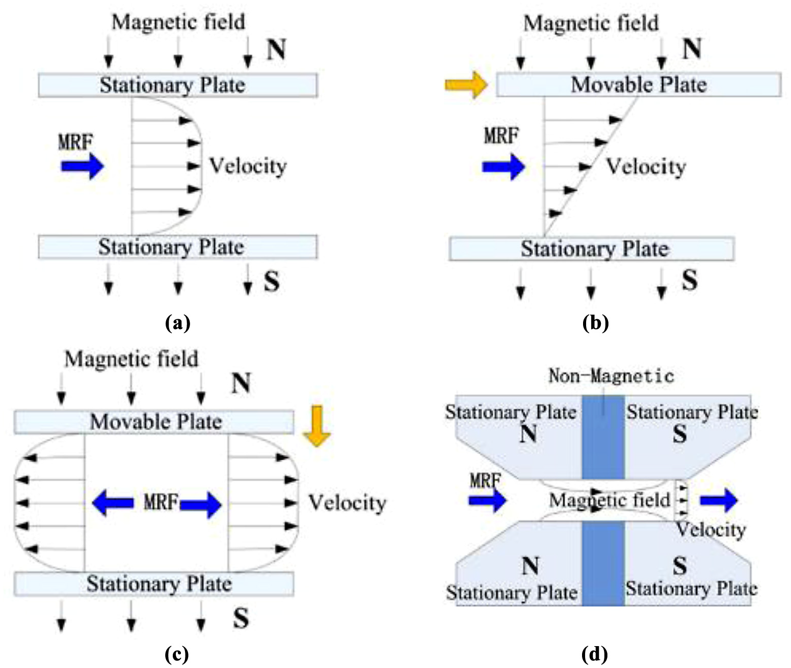
The schematic representations of the most common parametric models reviewed by Wang and Liao (2011) are shown in Figure 3. It can be shown that MR dampers are represented as nonlinear mechanical systems in which springs and dashpots configured in series and parallel connections are introduced. The models derived from the Bingham model, shown in Figure 3(a), are developed using modified configurations using springs, dashpots and other elements, as shown in Figure 3(b) to (e). These models were developed to predict the dynamic characteristics of MR dampers accurately. However, they employ more parameters whose values are required to be determined.
Schematic representations of parametric models of MR dampers reviewed by Wang and Liao (2011): (a) Bingham model (Spencer et al., 1997), (b) modified Bingham model (Zhou and Qu, 2002), (c) simple Bouc–Wen model (Spencer et al., 1997), (d) modified Bouc–Wen model (Spencer et al., 1997; Yang et al., 2013) and (e) viscoelastic–plastic model (Li et al., 2000).
The Bouc-Wen models, shown in Figure 3(c) and (d), are also widely used due to their robust performance in describing hysteretic behaviours of MR dampers. The simple Bouc-Wen model was initially developed by Bouc (1971) and later modified by Wen (1976). Currently, there are many modified model configurations based on the simple Bouc-Wen model. These models were developed for the accurate representation of the diverse hysteretic behaviours of MR dampers. Bai et al. (2015) used the phenomenological Bouc-Wen model shown in Figure 3(d), and derived other two models, which are called ‘normalised phenomenological’ and ‘restructured’ models, respectively. They employed a genetic algorithm to determine the parameters of each model, and they found that the new models have better accuracy and involve fewer parameters compared to the phenomenological Bouc–Wen model. Later, the same authors collaborated with Choi (Chen et al., 2018) to develop a novel hysteretic model, which employs a memory mechanism and a shape function. The memory mechanism was inspired from voltage charging and discharging processes in resistor–capacitor (RC) circuits, whereas the shape function provides more flexibility to the model. The new RC model was compared with the Bouc–Wen model when applying both models to investigate the hysteretic behaviour of an MR damper. It was found that the new RC model accurately predicts the output force of the damper and effectively reduces the computational time by 200% compared to the Bouc–Wen model. That reduction in computational time was due to the simpler equations adopted in the RC model. The RC model was also was compared with the Bouc–Wen and the restructured models by Bai et al. (2019), in which the relative errors between the models were analysed due to a wide range of frequencies and amplitudes of damper excitations.
Therefore, it can be inferred from the schematic representations shown in Figure 3 that the variables of the models given by stiffness,
In analytical models, the rheology of the fluid is only represented by the quasi-static analysis of fluid flow in the flow mode, shown in Figure 2(a), in which the dynamic effects are neglected. The dynamic rheological flow in MR dampers should have a mixed configuration between the flow and shear modes, represented by Figure 2(a) and (b), respectively (Elsaady et al., 2020; Syrakos et al., 2016). That is because the boundaries of the throttling area of the damper that represent the parallel surfaces in Figure 2(a) and (b) move in one direction as being a part from the piston, whereas, the fluid is throttled in the opposite direction. That causes the fluid layers adjacent to the walls of the throttling area to flow in the shear mode as a Couette flow, whereas the main part of flow is a Poiseuille flow exhibited by the valve mode (Elsaady et al., 2020).
The most common analytical models of MR dampers may include the following assumptions for the flow of MR fluid in the damper throttling area (Chooi, 2005; Chooi and Oyadiji, 2008, 2009; Çeşmeci and Engin, 2010): (1) incompressible, laminar and steady-state Poiseuille flow, (2) 1D axisymmetric flow with no velocity components in polar or radial directions, (3) the pressure variation is only with respect to the direction of flow, (4) the gravitational and inertial effects are neglected, and (5) the effect of the non-uniform distribution of magnetic field in the MR fluid region on the fluid viscosity is neglected. These assumptions are thought to sufficient for the determination of the quasi-static behaviour of MR fluids. However, the dynamic effects cannot be studied. It is worth to note that there are some analytical models in which the effects of fluid compressibility, transient analysis and inertial effects were considered, which indicates the importance of the inclusion of these effects (Bhatnagar, 2013; Chooi and Oyadiji, 2009).
2.2. Advantages of numerical models within MR dampers
Up to recent studies, modelling and analysis of MR dampers using numerical techniques is not frequently reported in comparison with analytical and experimental methods (Gurubasavaraju et al., 2018a; Syrakos et al., 2018). However, numerical methods are thought to be more effective than analytical models within MR damper research due to the reasons stated below. Paragraph (1) presents a general reason. Paragraphs (2) to (4) present the advantages attained by numerical electromagnetic models, whereas paragraphs (5) to (6) present the advantages achieved by numerical models of fluid flow.
Modelling of the multi-physics phenomena of MR dampers that combine electromagnetic, structural and fluid flow analyses is thought to be analysed in a more realistic way by a coupled numerical approach incorporated within a multi-physics numerical software, as shown in Case et al. (2013), Elsaady et al. (2020), Guo and Xie (2019), Gurubasavaraju et al. (2018a, 2018b), Parlak and Engin (2012), Parlak et al. (2012) and Zheng et al. (2017).
Within a numerical electromagnetic model, more parameters can be accounted for. Most importantly, the non-uniform distribution of magnetic field in the MR fluid region that represent the throttling area of the damper. Therefore, the effect of the non-uniform magnetic field on the fluid apparent viscosity can be studied (Case et al., 2013). The variable distribution of magnetic field density in the MR fluid region is shown in many studies (Case et al., 2013, 2014; Elsaady et al., 2020; Gurubasavaraju et al., 2018b; Singh et al., 2014; Yarali et al., 2019; Zheng et al., 2014). However, the coupled effect of that effect on fluid viscosity is not frequently seen.
Also, a transient numerical simulation can be included in the electromagnetic analysis. Therefore, a variable input current with time can be defined to the electromagnetic circuit. This is necessary to model the controllable behaviour of an MR device, in which the fluid is operated by a variable input current with time. The response time of the fluid to acquire the effect of magnetic field can be also included.
Moreover, numerical models offer modelling of the nonlinear properties of materials. Examples of these nonlinear properties are: nonlinear magnetic permeability, magnetic hysteresis, magnetic saturation and material non-homogeneity. The magnetic permeability of materials and MR fluids are usually considered as constant values in analytical and some numerical models (Chooi, 2005; Lee et al., 2018; Park et al., 2017; Syrakos et al., 2018). However, it is thought that the effect of nonlinearity of magnetic materials due to magnetic hysteresis and saturation is shown to be remarkable (Gołdasz, 2017).
Regarding the numerical fluid flow simulation, the outcome of applying numerical methods is thought to be more significant as it may give an insight into the characteristics of rheological fluid flow that cannot be predicted by analytical methods. Fewer model assumptions can be included in numerical models in comparison with those in analytical models. Therefore, a multi-dimensional transient flow of MR fluids can be solved instead of one-directional steady-state flow. The numerical analysis may also account for the effects of compressibility, gravity and fluid inertia, whereas most analytical models assume incompressible flow in which inertia and gravity effects are neglected.
Besides, numerical methods allow the study of MR fluid flow as a multi-phase flow rather than a single-phase. This allows the prediction of different phenomena manifested by MR fluids. For instance, Elsaady et al. (2020) studied the effect of the presence of air as a large pocket in MR dampers by the implementation of a numerical method. Potential studies may also include the effects of aeration and cavitation. It is worth to mention that there are two types of cavitation, namely, global and local cavitation (Kim et al., 2004). Numerical methods are worth to be used to study the local cavitation in which the models can be classified under four groups, namely: micro-bubbles dynamic models, interface tracking models, single-, and two-phase models (Sherman, 2016). Also, the multi-phase modelling of MR fluids may be applied in microstructure models in which the kinetics of ferromagnetic particles (solid phase) can be studied within a Lagrangian liquid–solid multi-phase flow.
Also, within a numerical flow analysis, the effects of more phenomena can be investigated. Examples of these parameters are the effects of temperature rise of MR fluids on apparent viscosity (Zheng et al., 2014), the response time of the fluid to acquire the apparent viscosity (Kubík et al., 2018) and turbulence effects.
One more important advantage, the strain and shear rate exerted by MR fluid during flow can be determined locally by numerical solvers of fluid flow. This allows the proper definition of fluid apparent viscosity as a function of the local strain and shear rate in order to accurately represent the viscoelastic-plastic behaviour of MR fluids.
Numerical techniques provide the different flow parameters to be visualised, which is important to analyse the flow characteristics. Examples of these parameters are pressure and viscosity contours, velocity vectors and fluid stream traces within the damper.
2.3. Challenges of a numerical approach for analysis of an MR fluid device
As presented in section ‘Advantages of numerical models within MR dampers’, study of MR fluid devices using numerical models is predicted to have many advantages. A coupled numerical modelling and analysis of an MR fluid device can be achieved mainly by performing a numerical analysis of the electromagnetic circuit and a fluid flow analysis of the flow field. The fluid properties in the flow model are defined according to the magnetic field applied.
Before reviewing the different pieces of research that investigate performances of MR fluid devices by numerical techniques, it may be necessary to illustrate the features of a numerical approach of an MR device. In other words, what are the aspects of a numerical model of an MR fluid device, so that the aforementioned advantages in section ‘Advantages of numerical models within MR dampers’ can be achieved? These features which were found to be challenging may interpret the few research pieces that investigate performance of MR fluids by numerical techniques. The aspects and/or challenges of this sort of coupled numerical approach can be summarised as follows:
A coupled fluid–structure interaction (FSI) is needed to investigate the MR fluid flow while being affected by magnetic field. The coupling strategy between both magnetic and fluid flow solvers should mainly define the fluid viscosity as a function of magnetic field density (intensity) and local shear rate. More additional considerations may be assumed in the definition of fluid viscosity in order to account for the effects of more parameters, such as fluid response time to acquire the effect of magnetic field, local strain and fluid temperature.
The theoretical viscoplastic equations, namely, the Bingham, Herschel–Bulkley and Casson models, which are the cornerstones of defining the fluid viscosity imply infinite viscosity at zero shear rates, as can be inferred from the constitutive equations of the models presented in Table 3. Therefore, these equations cannot be applied in numerical approaches, and other equations are necessary to be developed in order to be used safely in numerical techniques.
Regarding the fluid flow analysis, a transient simulation in a computational domain of an MR device is required. The domain may be open in some devices such as MR valves and pumps. Alternatively, it may be closed domain (no inlets or outlets) in many other applications such as MR dampers, journal bearings, rheometers and clutches. The convergence may be more difficult in closed domains, especially when a moving mesh technique is required as the mesh is updated in each time step. The moving mesh technique may be required to study the transient performance of some MR fluid applications, such as MR dampers in which the fluid is excited by the piston motion (Elsaady et al., 2020; Gołdasz, 2019).
The fact that not the whole fluid in an MR device may be affected by magnetic field. For instance, in MR dampers, the activated fluid only exists in the throttling area of the piston. However, the fluid in other locations of the damper is not affected by magnetic field. Therefore, the computational domain should adopt Newtonian zones which are not affected by magnetic field side by side with non-Newtonian yielded zones whose yield stress is variable. As a result, the viscosity of the fluid in the throttling area will be also variable.
In the following, previous research efforts on the preceding challenges are presented, namely, the coupling techniques between different numerical solvers, presented in (1), the definition of viscosity of viscoplastic fluids in numerical models, presented in (2), and the moving mesh techniques, presented in (3).
2.3.1. Coupling techniques
Referring to (1), the coupling techniques between the different solvers may be one- or two-way techniques. For an MR fluid application, a one-way coupling technique implies that the magnetic field domain is solved then the solution is exported to the fluid flow solver. On the other hand, in two-way coupling, the magnetic field is solved with the flow field simultaneously. FSI is frequently researched between structural and fluid flow analyses. However, fewer studies were shown to investigate a coupled solution between magnetic and fluid flow analyses, which is a special characteristic for ER, MR and ferro-fluids. The available pieces of research on coupled magnetic and fluid flow analyses are presented and criticised in sections ‘Numerical approaches applied to MR dampers’ and ‘Numerical approaches applied for MR applications other than MR dampers’.
Shams et al. (2007) employed a one-way coupling approach for an ordinary shock absorber filled with a Newtonian fluid. The structural analysis was conducted to determine the stresses on a deflector in the damper due to the fluid pressure attained from the fluid flow solver. If a two-way coupling approach is adopted by Shams et al. (2007), the deformation of the deflector, obtained with the structural analysis, will enlarge/shrink the volume of the fluid computational domain, solved by the fluid flow solver. It is believed that two-way FSI is obligatory to be considered for some applications, especially in micro-scale devices, such as micro-pumps (Longo et al., 2017), or where the elasticity of the solid parts are considered as in biomedical blood simulation in veins (Ibrahim et al., 2017). However, FSI may be an unnecessary sophistication if it employed where the fluid domain is too large compared to the deformation of the solid bodies.
2.3.2. Defining the non-Newtonian viscosity in numerical techniques
Referring to the incompatibility of theoretical viscoplastic models in numerical approaches mentioned in (2), different alternative functions were developed to define the viscosity of yielded fluids in numerical models. Some of these functions were reviewed by Mitsoulis (2007) and other functions are shown in Case et al. (2013), Choi et al. (2005), Susan-Resiga (2009) and Zheng et al. (2015). According to Mitsoulis (2007), earlier models were introduced by Bercovier and Engelman (1980), Taylor et al. (1983), Glowinski (1985) and Beris et al. (1985). However, the most common model was introduced by Papanastasiou (1987). In Papanastasiou’s model, an exponential function was proposed by introducing a new parameter,

whereas the Herschel–Bulkley–Papanastasiou and the Casson–Papanastasiou models have the following forms, respectively

Choi et al. (2005) presented a two-parameter viscoplastic model, termed as ‘Eyring model’. The shear stress is defined according to that model as shown in equation (7). The use of the Eyring model is thought to be not reported in numerical methods of MR fluid applications. However, it has been used recently by Tošić et al. (2019) to define the rheological behaviour of a lubricant within a CFD model

where
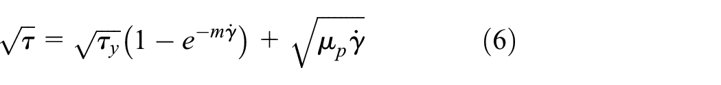
Susan-Resiga (2009) developed a numerical model that incorporates the quasi-Newtonian behaviour of Herschel-Bulkley fluids at very low shear rates with the viscous behaviour occurs at relatively higher shear rates. The model included a mathematical relation that was developed using hyperbolic tangent functions to define the shear stress, as shown in equation (8). The study also compared different mathematical relations in the forms of error and exponential functions. The models were validated by the experimental measurements of the shear stress – shear rate diagram of MRF-132DG MR fluid, produced by LORD Corporation, at different magnetic field strengths
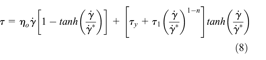
where
Using a hyperbolic tangent function also, the non-Newtonian viscosity of yielded fluids was defined by Case et al. (2013), (2014) and Zheng et al. (2015) as
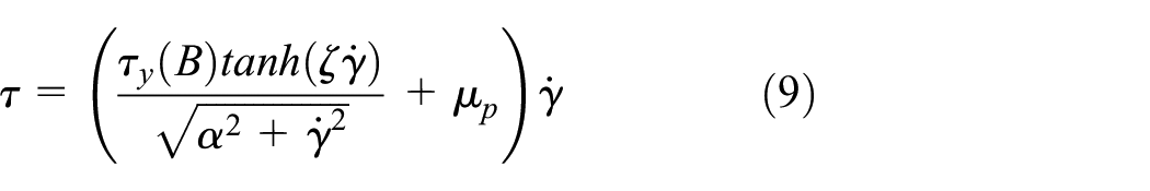
where
The previous constitutive equations shown by equations (4)–(9) define the shear stress of yielded fluids by a single equation. This leads to avoiding discontinuities in the viscosity definition (Taibi and Messelmi, 2017). On the other hand, a bi-viscous definition is also employed in order to implement the same theoretical viscoplastic equations, presented in Table 3, in numerical techniques. In bi-viscous constitutive equations, a maximum value of viscosity is assigned at a critical shear rate. Therefore, the non-Newtonian viscosity is defined in Bingham bi-viscous model as
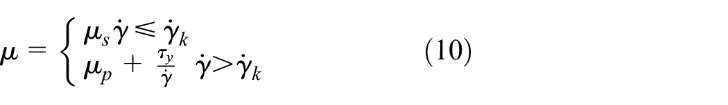
where
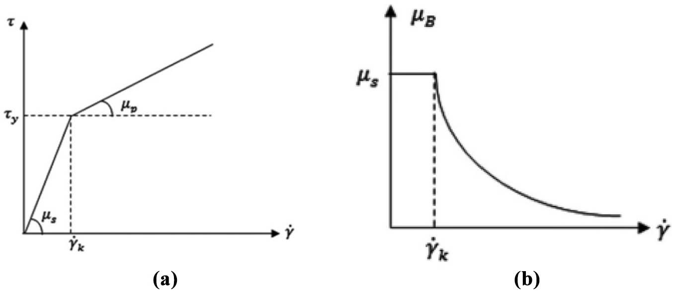
Schematic representations of the bi-viscous Bingham model (Bullough et al., 2008): (a) flow curve and (b) viscosity profile.
The bi-viscous approach is adopted, for example, in the built-in library for generalised Newtonian and viscoplastic fluids in ANSYS/Fluent software (2009). The generalised Newtonian fluids are un-yielded non-Newtonian fluids. They are termed as ‘generalised Newtonian fluids’, as the constitutive equations of these fluids are generalised by modifying the linear flow equation of Newtonian fluids to a nonlinear equation (Saramito, 2016). The built-in library in ANSYS/Fluent software allows determination of the fluid shear-rate-dependent viscosity according to the power-law, the Carreau model, the Cross model or the Herschel-Bulkley model. The first three models are developed for generalised Newtonian fluids, whereas the Herschel–Bulkley model is developed for viscoplastic fluids, and also it can represent Bingham plastic model if the flow index,
The profiles of the constitutive equations shown by equations (4)–(10) are quite different. This helps on the proper selection of the equation and parameters which match the rheological characteristics of the employed MR fluid in each study. The profiles of different constitutive equations are compared with the theoretical Bingham relation, as shown in Figure 5. Hypothetical values of yield stress and plastic viscosity, taken as
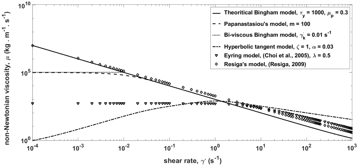
Definition of the non-Newtonian viscosity of yielded fluids with different flow functions, for hypothetical values of yield stress and plastic viscosity, taken as:
2.3.3. Moving mesh
Referring to (3), one of the challenges of transient numerical simulations is the need to update the mesh due to the motion of boundaries in some of these simulations. For instance, a moving mesh technique is required to develop a transient simulation of flow field in MR dampers. The mesh must be updated in each time step to simulate the movement of the piston.
Different moving mesh techniques are included in most numerical software. These techniques define the conditions at which the mesh is changed. It should be noted that not all of these techniques are included in all software. The most common moving mesh techniques, namely layering, smoothing and remeshing techniques are included in ANSYS/Fluent (2009). The Layering method in ANSYS/Fluent adds or removes cells adjacent to moving boundaries. The moving boundaries can be walls or fluid zones. It is valid only for quadrilateral cell shapes in two-dimensional (2D) problems, or wedge and hexahedron cell shapes in 3D problems. The transient CFD simulations of flow in MR dampers presented by Elsaady et al. (2020) and Gołdasz (2019) adopt this technique.
In smoothing technique, no cells are deleted or created during mesh update. The locations of some or all nodes are changed based on a pre-defined regime, which keeps the original basic shape of the mesh. The pre-defined regime may be based on a spring action, in which the nodes of the mesh are treated as a network of interconnected springs. Also, an alternative method, termed as Laplacian method, allows the update of node locations only if the maximum skewness of all faces is improved in comparison with the old mesh. The third regime of smoothing technique is termed as the boundary layer method, which is applied to preserve the boundary layer thickness adjacent to a moving or rotating moving boundary. The fourth approach is the diffusion-based smoothing method in which the nodes are moved according to a pre-defined equation based on the velocity of the moving boundaries. The smoothing methods are also the methods adopted in COMSOL/Multiphysics (COMSOL, 2018).
In remeshing technique, new cells are added or removed based on a pre-defined condition of all cells in the mesh. For instance, the mesh is modified if the values of skewness or cell size of some cells exceed a pre-defined maximum value or be lower than a critical minimum value.
2.4. Methods of numerical analysis
FEM, FDM and FVM are the classical numerical methods applied for discretising a system of partial differential equations (PDEs). The discretised equations are solved within a computational domain represented by a mesh composed of a number of nodes and cells (Peiró and Sherwin, 2005). The FDM is the oldest method which applies a local Taylor expansion to discretise the differential equations on structured grids. To allow more flexibility of discretisation techniques in complex geometries, FE and FV methods were developed (Wikipedia, 2001). FE and FV methods are based on the integral forms of PDEs, whereas, FDM discretises the differential forms.
The main difference between FEMs and FVMs is that the quantities in FVMs are cell-averaged values, whereas in FEMs and FDMs, the values are localised at the mesh points (Hirsch, 2007). Therefore, FEMs and FVMs can be distinguished by the following two features (Blazek, 2015):
The coordinates of the mesh points do not appear in FVMs unless for the determination of the cell volume and side areas. Consequently, the physical property is not attached to a specific point inside the control volume (cell) and can be considered as an average value over the control volume.
In the absence of source terms in PDEs, FVMs assume that the variation of the average value of a physical property over a time interval equals to the sum of the fluxes exchanged between neighbouring cells. In other words, the conservation laws of FVMs assume that physical quantities that go into a cell side need to leave the same cell from other sides.
2.4.1. Implementation of FVMs and FEMs in structural and fluid flow analyses
It is commonly agreed that FVMs are more suitable for simulations of fluid flows compared to FEMs, and FEMs are more suitable for structural analysis (Hirsch, 2007). Although that does not mean that FEMs are not suitable for investigation of fluid flows. The FEMs of fluid flow problems are introduced in many literatures (Donea and Huerta, 2003; Tezduyar, 2001; Zienkiewicz et al., 2014). Moreover, some comparisons between the two approaches in different fields of structural and fluid simulations are presented (Abali, 2019; Fallah et al., 2000; Jeong and Seong, 2014; Lukáčová-Medvid’ová and Teschke, 2006; Molina-Aiz et al., 2010; O’Callaghan et al., 2003). The analysis of these pieces of research asserts the common thought of the more suitability of FVMs in fluid flow problems in terms of accuracy, numerical stability and speed of calculations, as will be shown below.
The FE and FV methods were applied by Molina-Aiz et al. (2010) for the simulation of air flow in ventilation of greenhouses. The FE model was shown to allow easier meshing compared to the FV model. However, the computational time required for the solution of the FE model was twice longer than that of the FV model. Moreover, the FE model required 10 times greater storage memory compared to the FV model. The authors attributed this to the different computation procedures used by each scheme.
The same observations of the greater computational time and storage memory required by FE models were also stated by Jeong and Seong (2014), and Lukáčová-Medvid’ová and Teschke (2006). Jeong and Seong (2014) compared two FVM-based commercial CFD solvers with an FEM-based solver to analyse fluid flow in simple and Y-shaped pipes. The CFD models were developed using ANSYS/Fluent and ANSYS/CFX, whereas the FEM solver used was ADINA. It was shown that the calculation time needed for the same mesh size of the fluid domain is approximately five times greater in the FEM-based model in comparison with the two FVM-based models. Moreover, the FEM-based model was shown to be more affected by mesh type and quality compared to the FVM-based model. In Lukáčová-Medvid’ová and Teschke (2006), FE and FV simulations were implemented to analyse the flow of water in channels with different shapes. It was analysed that the FV model was more efficient and faster than the FE model. Recently, an FE model has been developed for an isothermal incompressible turbulent flow of a viscous fluid in pipes (Abali, 2019). The method was described as ‘challenging’ due to the problems encountered in terms of numerical stability, accuracy and convergence.
O’Callaghan et al. (2003) applied the FE and FV methods to investigate blood flow in artery. The authors found that both methods gave accurate results in comparison with the theoretical Poiseuille flow analysis. The FVM, implemented via ANSYS/Fluent led to more accurate results. However, it required double computational time and storage memory compared to the FE analysis. The reason for that is because the number of cells in the FV model was higher than that in the FE analysis.
On the other hand, FEMs were shown to be better than FVMs for investigations in structural mechanics. An FV model for the analysis of geometrically nonlinear problems based on the Lagrangian approach was developed using FORTRAN by Fallah et al. (2000). The FV model was shown to have a good accuracy compared to another FE model. However, the better accuracy of the FV model was only obtained when a higher mesh density compared to the FE model, which required more calculation time and storage memory. FVMs were also shown to be used in structural mechanics in some particular cases due to the advantages of less computational time (Idelsohn and Oñate, 1994; Onate et al., 1994; Wenke and Wheel, 2003; Zienkiewicz et al., 2014). It is thought that the main reason for the employment of FEMs in structural mechanics is the greater accuracy of FEMs due to the employment of Galerkin optimal approximations for self-adjoint problems, which are not employed in FVMs (Idelsohn and Oñate, 1994; Onate et al., 1994; Zienkiewicz et al., 2014). Therefore, FVMs can be compared to FE analysis performed with non-Galerkin weighting (Onate et al., 1994).
Through the preceding analysis of the implementation of FVMs and FEMs in structural and fluid flow analyses, it can be said that FVMs are thought to be more suitable for modelling and simulation of MR fluid flow, whereas FEMs are more suitable for electromagnetic simulation. However, FEMs may also lead to good results for MR fluid flow in creeping conditions which occur at very low flow velocities. That is because, the effects of convective acceleration (rate of change of flow velocity due to the change of position of fluid particles) are negligible (Zienkiewicz et al., 2014). It should be noted that the effects of convective acceleration cause the flow equations to be non-self-adjoint problems, which affects the stability of the solution if the Galerkin method employed by FEMs is used (Zienkiewicz et al., 2014). The creeping conditions are employed in some MR devices in which the loading conditions are minor. However, there is no complete judgement on the suitability of FVMs and FEMs in MR fluid research. It is thought that the only way for a fair judgement is to employ both methods to investigate the performance of an MR device under different flow conditions but identical mesh sizes. Thus, the stability of solution, computational time and computer storage requirements will be assessed for both methods. In the light of the analysis of the preceding literature, it is expected that the results of FEMs of fluid flow will be comparable with FVM solutions in terms of stability and computational speed, as long as the flow tends to be steady. However, it is thought that FEMs will be challenging to use for transitional and turbulent flows.
3. Reviewing research efforts on modelling MR fluid devices via numerical approaches
In the following, different research papers that investigate MR fluid devices using numerical techniques are reviewed. The review will show the applications in which MR fluids are employed, characteristics of both magnetic and fluid flow solvers, coupling strategies between the solvers, and how the fluid viscosity is defined in the numerical model of each study. This information is summarised in Table 4, which shows the discretisation techniques used and the commercial solvers employed for both magnetic and fluid flow fields.
Research on modelling and simulation of MR fluids using numerical approaches.
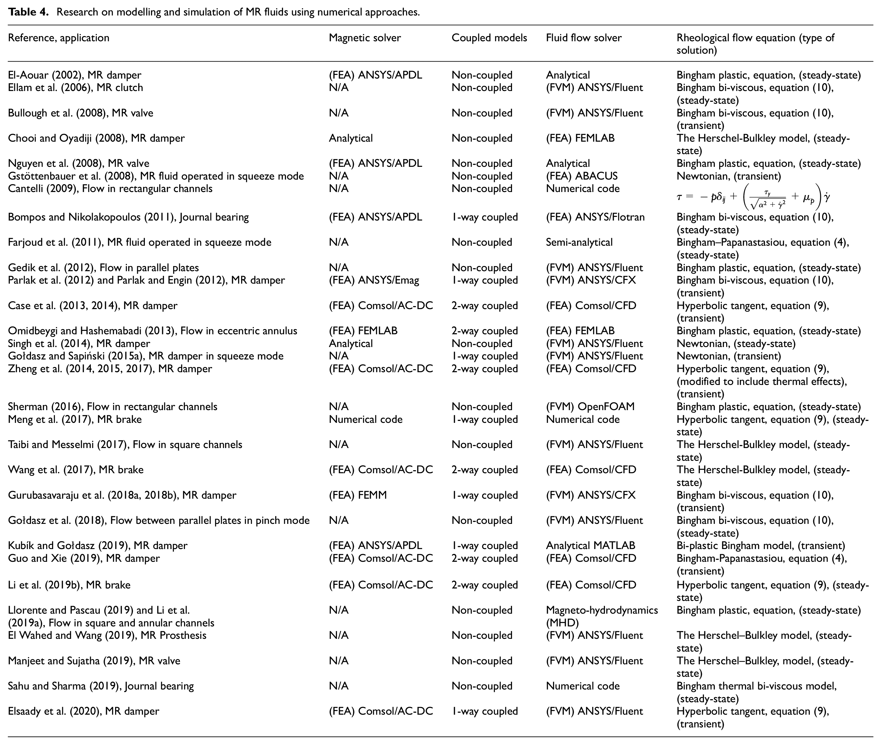
It can be seen from Table 4 that numerical investigations of MR devices have attracted more interest in the last 10 years. The reason for that is thought to be due to continuous enhancements of numerical solvers available in commercial software. The magnetic solvers are mostly implemented by FEA in different commercial solvers such as ANSYS/Emag, ANSYS/APDL, ANSYS/Maxwell, and COMSOL/Multi-physics. However, the solvers of fluid flow are diverse, as they include FE- and FV-based methods using various solvers and different conditions and assumptions. Also, the table shows that the majority of the papers reviewed applied either the hyperbolic tangent or the Bingham bi-viscous constitutive equations, defined by equations (9) and (10), respectively, in order to define the rheological flow behaviour. It can be also seen that transient flow field models are relatively fewer compared to the steady-state models.
Table 4 also shows whether the presented models are one-way, two-way, or non-coupled models. The one-way coupling techniques are shown to be adopted in FEM-based magnetic field simulation coupled with FVM-based flow analysis, as shown by Elsaady et al. (2020), Gołdasz and Sapiński (2015a), Gurubasavaraju et al. (2018a, 2018b), Meng et al. (2017), Parlak and Engin (2012) and Parlak et al. (2012). The two-way coupled solutions are often to be performed by COMSOL/Multiphysics in which the AD/DC module is used for magnetic field simulation, whereas the fluid flow and heat transfer modules are used for fluid flow solution, as shown by Bompos and Nikolakopoulos (2011), Case et al. (2013, 2014), Guo and Xie (2019), Li et al. (2019b), Omidbeygi and Hashemabadi (2013), Wang et al. (2017) and Zheng et al. (2014, 2015, 2017). The non-coupled solutions are found where the magnetic field solution was not investigated, as by Bullough et al. (2008), Cantelli (2009), Ellam et al. (2006), Gedik et al. (2012), Gołdasz et al. (2018), Gstöttenbauer et al. (2008), Li et al. (2019a), Llorente and Pascau (2019), Manjeet and Sujatha (2019), Sahu and Sharma (2019) and Taibi and Messelmi (2017), or was implemented by analytical solutions, as shown in Chooi and Oyadiji (2008) and Singh et al. (2014).
In comparison with numerical flow field models, the numerical magnetic field models are more frequent to be seen in MR fluid research, either as stand-alone models or together with analytical fluid flow equations (Ding et al., 2013; Dong, 2016; El Wahed and Balkhoyor, 2017; Gao et al., 2017; Gołdasz and Sapiński, 2017; Hong et al., 2015; Kim et al., 2016b; Li et al., 2017; Nanthakumar et al., 2019; Ouyang et al., 2015; Paul et al., 2014; Yu et al., 2016).
The review of the research papers shown in Table 4 is organised in the following two sections. Section ‘Numerical approaches applied to MR dampers’ presents the analysis of numerical approaches applied to MR dampers, whereas section ‘Numerical approaches applied for MR applications other than MR dampers’ shows the numerical approaches applied to other MR applications. The governing equations and the improvements attained due to the employment of numerical models rather than analytical models are presented. Moreover, the capabilities and limitations of these models are evaluated and criticised.
4. Numerical approaches applied to MR dampers
This section presents the analysis of numerical approaches applied to MR dampers. The analysis of numerical approaches applied to other MR fluid devices is presented in section ‘Numerical approaches applied for MR applications other than MR dampers’. The contents of the current section are divided into two subsections; section ‘Modelling and simulation of magnetic circuit of MR dampers’ presents the numerical approaches applied for magnetic circuit analysis, whereas section ‘Modelling and simulation of flow field in MR dampers’ presents the numerical approaches applied for fluid flow analysis. Each subsection starts with presenting the main governing equations, then the relevant pieces of literature are criticised showing the main characteristics and improvements attained by employing numerical techniques.
4.1. Modelling and simulation of magnetic circuit of MR dampers
4.1.1. Governing equations of magnetic field
The magnetic circuit of an MR damper is represented by the piston head, where the coils are located. MR pistons are usually composed of an inner and an outer part. Coils are usually wound on the inner part of the piston. A schematic drawing of an MR piston containing a single coil and the representation of magnetic circuit is shown in Figure 6. The figure shows that magnetic flux flows in a loop around the coil section. The analytical solution of flow of magnetic flux is based on Ampere’s and Kirchhoff’s laws, in which the magnetic circuit is represented by an electric circuit composed of a number of reluctances (Wikipedia, 2003). Each reluctance represents the magnetic resistance to the flow of magnetic flux in each uniform medium. The summation of the reluctances represents the total magnetic resistance of the magnetic circuit. Hence, the static magneto-motive force,
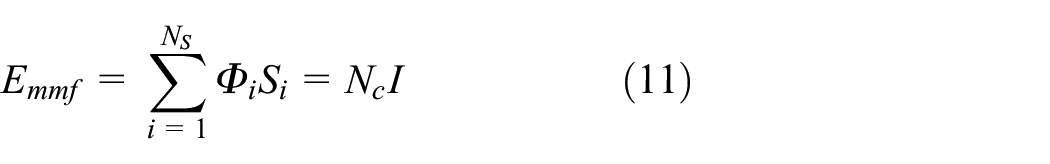
where
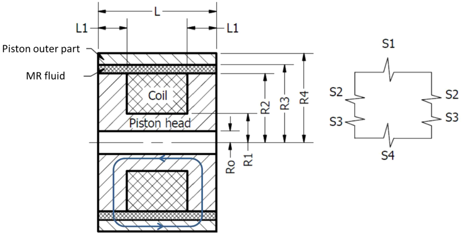
Construction and analytical representation of a magnetic circuit of an MR damper.
The values of the reluctances,
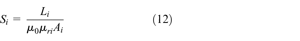
where
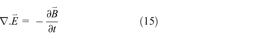
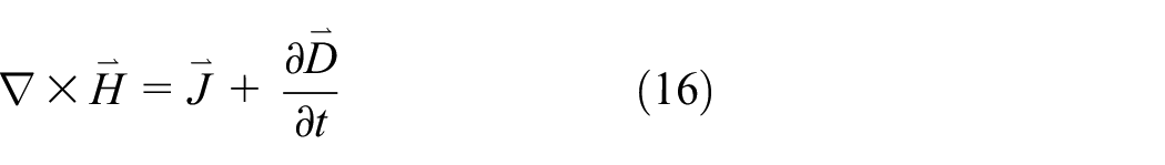
The electromagnetic field in different MR fluid applications is governed by Maxwell’s equations. Maxwell’s equations are composed of a set of four differential equations that form the theoretical basis of classical electromagnetism by setting the relations between the fundamental quantities (Purcell and Morin, 2013). These quantities are electric field intensity,


Other additional constitutive relations between different electromagnetic quantities are employed in numerical solutions to obtain a closed system of equations. For instance, the following additional equations are used in COMSOL/Multiphysics solver (COMSOL, 2018), to interpret continuity and macroscopic properties of the medium


where
4.1.2. Improvements of numerical analysis of magnetic circuits of MR dampers
The theoretical analysis using magnetic Kirchhoff’s law is a static one, which determines the average magnetic field over the magnetic circuit. For MR dampers, the theoretical analysis could be useful as a quick check for dimensions and material selection for MR dampers. However, it does not predict the variable distribution of magnetic field in the damper that can be predicted by the solution of Maxwell’s equations. Thus, the numerical models of magnetic circuits of MR dampers can predict more parameters, namely (1) the non-uniform distribution of magnetic field in the MR fluid region, (2) prediction of the nonlinear magnetic characteristics due to magnetic hysteresis and saturation, (3) implementation of design optimisation of magnetic circuits of MR dampers, and (4) investigation of response time of MR fluids to acquire the effect of magnetic field.
4.1.2.1. The non-uniform distribution of magnetic field in the MR fluid region
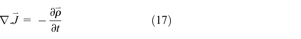
The prediction of the non-uniform distribution of magnetic field in the MR fluid region which affects the apparent viscosity of the MR fluid is thought to be the main outcome of numerical simulations of magnetic field. Magnetic flux flows mainly from the farthermost ends of the piston (magnetic poles) and intermediate magnetic spacers if more than one coil is used, as shown in Figure 7. However, the magnetic flux decays in the MR fluid regions that are adjacent to the coils. This variable distribution of magnetic field density/strength leads to a variable yield stress of the fluid along the MR fluid region. Thus, the effect of this variable distribution on fluid viscosity is the cornerstone of a coupled analysis, as will be shown in section ‘Coupling between magnetic and fluid flow solvers’.
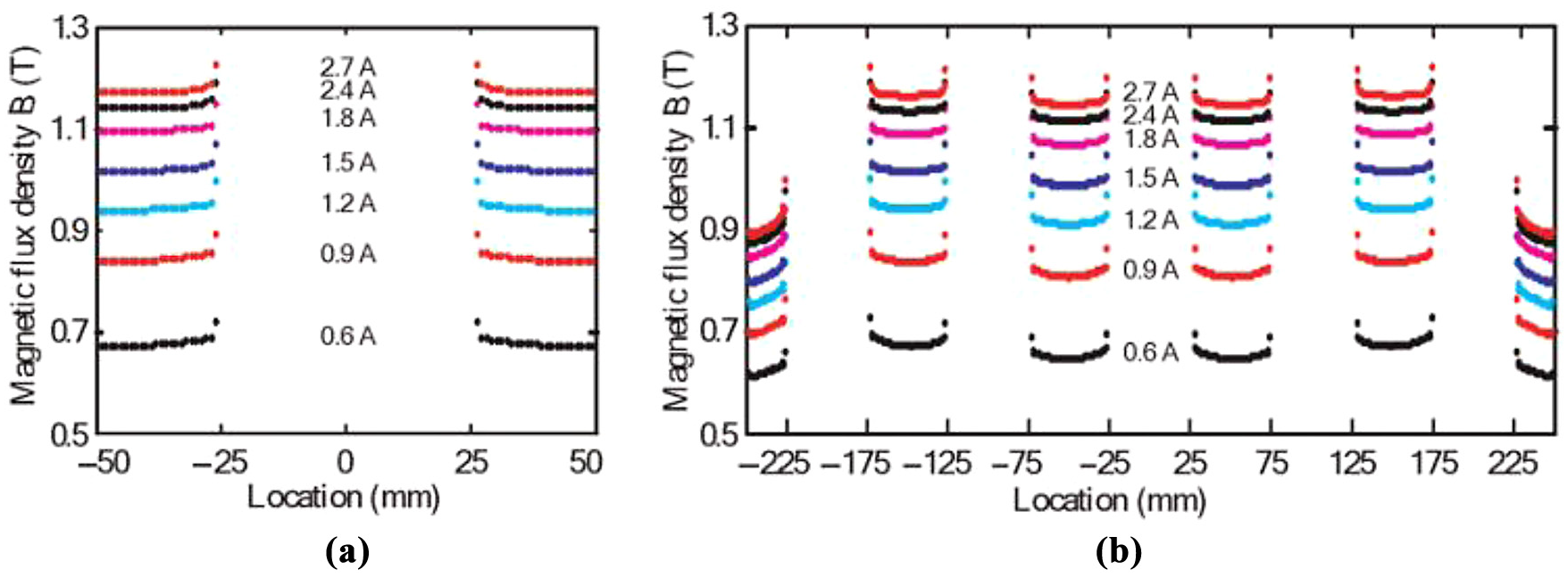
Variable magnetic field distribution in MR fluid region in MR dampers (a) magnetic field density employing four coils (Zheng et al., 2015) and (b) magnetic field strength employing five coils (Singh et al., 2014).
El-Aouar (2002) developed a 2D axisymmetric model based on FEA for the magnetic circuit analysis of an MR damper using ANSYS/APDL. Four constructions of the MR damper piston were studied in which the magnetic field density and the damper force were predicted for each construction. The most advantageous construction was identified based on the evaluation of damper force and power consumption. The damper force was predicted by an analytical model, in which the average value of magnetic field density obtained from the FE model was used to define the fluid yield stress in the analytical model.
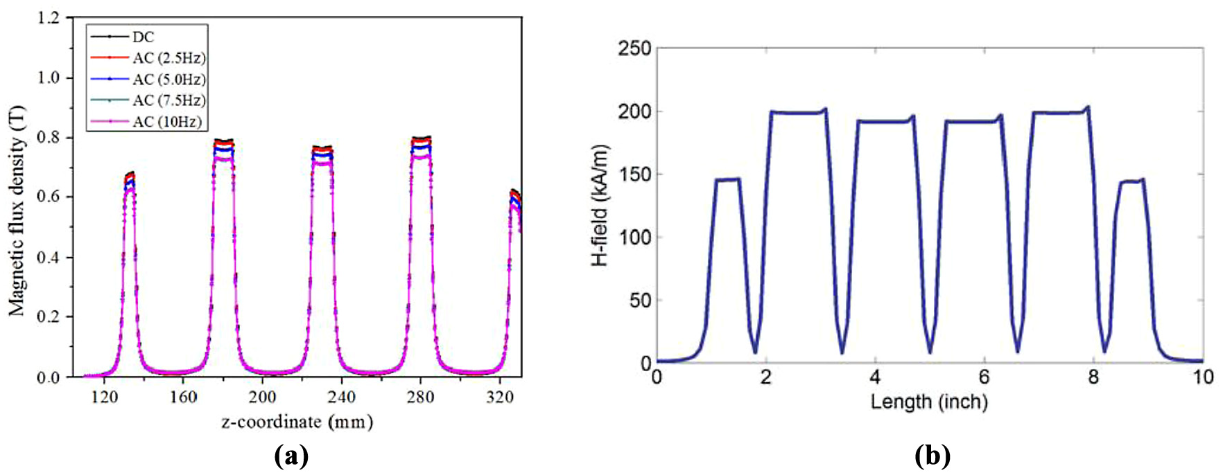
Kim et al. (2016b) presented a new design of an MR damper with a bi-fold flow gap in order to improve the damping performance. The MR fluid path in the piston permits the fluid to flow around the outer surface of the coil bobbin, and also inside the coil core, as shown in Figure 8(a). They adopted this construction as the magnetic streamlines are expected to be denser in the coil core. Thus, the magnetic effect on the MR fluid increases. As can be seen in Figure 8(b), the distribution of magnetic flux density in the inner zone is approximately twice greater than that in the outer zone. The FE model was implemented by ANSYS/Emag software, whereas an analytical solution of the fluid flow was presented.
Modelling of an MR damper with bi-fold flow gap shown by Kim et al. (2016b): (a) construction of the piston and (b) distributions of magnetic field strengths in the inner and outer fluid regions.
4.1.2.2. Inclusion of nonlinear magnetic properties and magnetic hysteresis
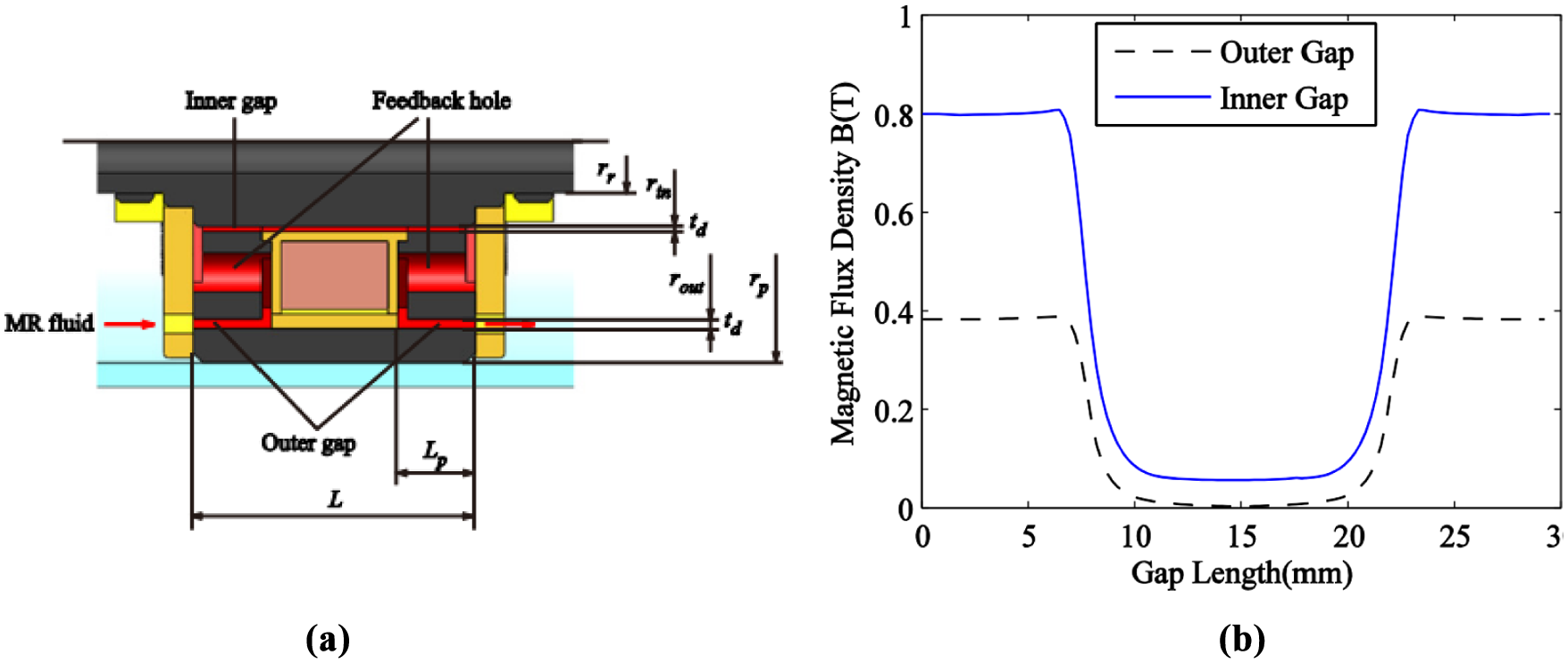
Magnetic field is a nonlinear phenomenon which is affected by magnetic saturation and hysteresis. Although MR dampers operate at low operation currents, the dampers may be liable to magnetic saturation (Gołdasz, 2017; Xu et al., 2012). The relative permeability of magnetic materials and MR fluid are assumed in some models by constant values (Chooi, 2005; Lee et al., 2018; Park et al., 2017; Paul et al., 2014; Syrakos et al., 2018). However, it is thought that the relative permeability should be defined according to the
Predictions of the distribution of magnetic flux densities in MR fluid region of an MR damper presented by Xu et al. (2012): (a) single-coil piston and (b) multi-coil piston employs five coils.
Apart from nonlinearity caused by magnetic saturation, there is another source of nonlinearity caused by magnetic hysteresis. Magnetic materials exhibit a hysteretic
Determination of the hysteretic
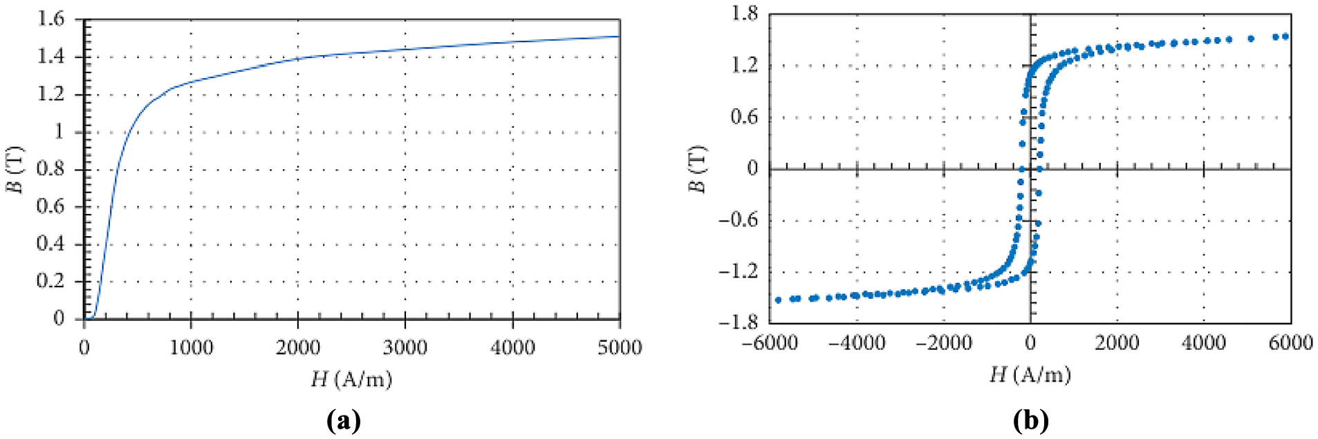
(a) Stationary and (b) hysteretic
4.1.2.3. Design optimisation of magnetic circuits of MR dampers
Modelling and simulation of magnetic circuits of MR dampers by FE models allow design optimisation of the parameters of magnetic circuit (Yu et al., 2016; Zheng et al., 2017). Zheng et al. (2017) presented a multi-physics optimisation model of a novel MR damper with multi-coil configuration and a variable thickness of the throttling area of the piston. The objective function of the optimisation problem was to determine the optimal geometrical dimensions of the throttling area, whereas the parameters were the total damping force of the damper, dynamic range and the inductive time constant. The inductive time constant is the time needed for electric current flowing in an electromagnetic circuit to reach 63.2% of its steady-state value. An FE multi-physics optimisation model was developed using COMSOL/Multiphysics software in which the magnetic and flow field analyses are performed. The dynamic characteristics of the MR damper with the optimised variable throttling area were compared with those of an MR damper with constant throttling area. The comparison shows that the performance of the MR damper with optimised variable throttling area has significant improvements in terms of increasing output force of the damper and decreasing the inductive time constant.
Yu et al. (2016) developed an FE optimisation model of a rotary MR damper. The objective function of the optimisation problem was to determine the maximum output damping torque of the damper. An FE model of the damper magnetic circuit was solved using ANSYS/APDL software, in conjunction with an analytical model of the fluid flow developed with MATLAB. The optimal design was used to fabricate a novel rotational MR damper which was tested at low and high rotational speeds in order to measure the damping torque. A good matching between theoretical and experimental results was achieved in terms of the maximum values of the torque. However, the accuracy is not so high at the moments of maximum angular velocity. That is due to the quasi-static analytical model employed.
4.1.2.4. Investigation of response time of MR fluids to magnetic field
Response time of MR fluids to acquire magnetic effect in MR dampers is an important design parameter which affects the performance of damper, especially when the damper is driven by an automatic control circuit with variable input current (Kubík et al., 2018). Experimental measurements of the transient response of MR fluids due to step input of electric current are found in many studies (Chooi and Oyadiji, 2005; Kubík et al., 2018). Kubík et al. (2018) developed a 2D transient FE model for the magnetic circuit of an MR damper using ANSYS/APDL software. They validated their model by experimental measurements of the magnetic field density in the MR fluid region using a measuring circuit that employs a Hall-effect sensor. The effect of volume fraction of ferromagnetic particles on the fluid response time was studied. It was found that the lower concentration of ferromagnetic particles leads to a faster response of the MR fluid to magnetic field.
4.2. Modelling and simulation of flow field in MR dampers
After the preceding analysis of the improvements that attained due to applying numerical methods in magnetic circuit analysis for MR dampers, a similar analysis is presented in this section for fluid flow. The methodologies applied in the literature for numerical modelling and simulation of flow field in MR dampers under cyclic loads are presented. In the available literature to the authors, studies that employ numerical modelling and simulation of fluid flow fields in MR dampers are found to be relatively fewer in comparison with those that employ numerical magnetic field simulation or analytical flow field modelling. Moreover, the methods applied in numerical flow field simulation are diverse as presented in Table 4. The research papers that apply numerical flow field simulations of MR dampers were found in Case et al. (2013, 2014), Elsaady et al. (2020), Gołdasz (2019), Guo and Xie (2019), Gurubasavaraju et al. (2018a, 2018b), Kemerli et al. (2018, 2019), Li et al. (2019a), Manjeet and Sujatha (2019), Parlak and Engin (2012), Singh et al. (2014), Syrakos et al. (2016) and Zheng et al. (2014, 2015).
An MR damper shows a hysteretic behaviour that can be shown in the force–velocity diagram when subjected to cyclic loads. The force–velocity diagram is denoted as ‘characteristic diagram’, which is used in conjunction with the force–displacement diagram, denoted as ‘work diagram’, in order to describe the dynamic performance of an MR damper subjected to cyclic excitations. Modelling the sources of this hysteretic behaviour is thought to be the key factor of the prediction of nonlinear behaviour of MR dampers under cyclic loads. That is why the dynamic models developed for MR dampers are more preferred to quasi-static models (Wang and Liao, 2011).
However, among the aforementioned research papers that apply numerical flow field simulations of MR dampers under cyclic loads, the characteristic diagrams obtained from the numerical methods used are not shown, except for references (Elsaady et al., 2020; Guo and Xie, 2019; Kemerli et al., 2018, 2019; Syrakos et al., 2016). The characteristic diagrams are shown by Kemerli et al. (2018, 2019) and Syrakos et al. (2016). However, the hysteretic behaviour that was shown in the experiments was not predicted by the models developed by Kemerli et al. (2018, 2019). Also, the theoretical results are only shown by Syrakos et al. (2016). In Elsaady et al. (2020), the hysteretic behaviour of the damper was modelled based on modelling of the effects of fluid compressibility and the presence of an air pocket, whereas in the study by Guo and Xie (2019), it was modelled based on the effects of fluid compressibility and viscoelasticity. The detailed analysis of the methods employed in these papers is presented in this section.
The subsequent sections present the main governing equations of fluid flow in MR dampers in section ‘Governing equations of flow field’. Then, the analysis of the available aforementioned literature is presented in section ‘Coupling between magnetic and fluid flow solvers’ to ‘Analysis of nonlinear behaviour of MR dampers by numerical fluid flow solvers’. Section ‘Coupling between magnetic and fluid flow solvers’ presents the coupling techniques; Section ‘Predictions of the rheological behaviour of MR fluids (velocity and shear rate)’ presents the predictions of the rheological behaviour of MR fluids predicted by numerical models, in terms of velocity and shear rates; section ‘Predictions of apparent viscosity in numerical fluid flow models’ presents the predictions of viscosity which is the coupled parameter between the two solvers. Finally, section ‘Analysis of nonlinear behaviour of MR dampers by numerical fluid flow solvers’ presents the analysis of the nonlinear behaviour of MR dampers, which shows that most of the numerical models developed in the available literature were incapable to predict the hysteretic behaviour of MR dampers due to the complexity of modelling the flow behaviour and the assumptions included in the models.
4.2.1. Governing equations of flow field
The flow of MR fluids in different MR devices is governed by the well-known continuity and Navier–Stokes equations, given as (Elsaady et al., 2020; Guo and Xie, 2019)

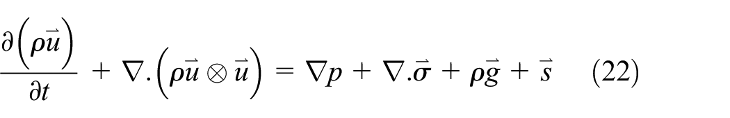
where
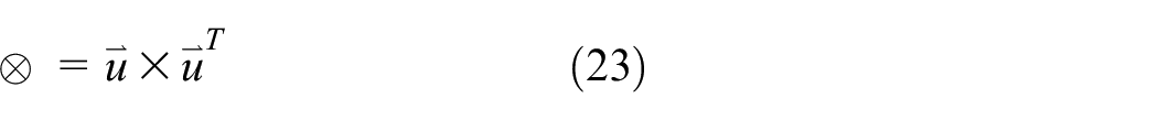
To model the fluid flow in MR dampers, the continuity and Navier–Stokes equations are defined in cylindrical coordinates, in which the tangential components of parameters do not exist in 2D analyses. The flow equations are discretised in the integral form to be implemented in numerical solvers.
The fluid inertia and compressibility are included in the momentum equation by the term
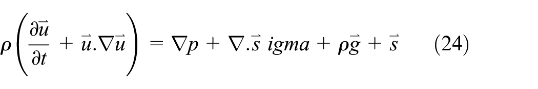
The source term,
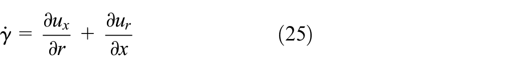
where
The laminar flow condition was verified according to the conditions applied for the piston movement in the reviewed research papers that investigated numerical modelling and simulation of MR fluid flow in MR dampers under cyclic loads. 2D flow field simulations are presented by Case et al. (2013, 2014), Elsaady et al. (2020), Guo and Xie (2019), Singh et al. (2014) and Zheng et al. (2014, 2015), whereas three-dimensional (3D) simulations are presented by Gurubasavaraju et al. (2018a, 2018b) and Parlak and Engin (2012).
4.2.2. Coupling between magnetic and fluid flow solvers
The one- and two-way coupling techniques between magnetic and fluid flow solvers are reported in available literature. The two-way coupling technique is only reported to be implemented by COMSOL/Multiphysics by Case et al. (2013, 2014) and Zheng et al. (2014, 2015). However, different decoupled and one-way coupling methods were reported, as shown in Table 4. The equations applied to define the apparent viscosity in order to perform coupling are also shown in Table 4.
COMSOL/Multiphysics provides an integrated FE multi-physics software environment in which coupled physics phenomena are solved together in the same solver (COMSOL, 2018). Solution of coupled physics is also provided and continuously upgraded in ANSYS software. However, the solution is implemented by different solvers and the coupling is implemented by ANSYS/Workbench which is the workflow analysis platform of ANSYS software. Therefore, ANSYS/Workbench gives more flexibility to apply different FE- and FV-based solvers for each domain but also requires a special setup between the coupled parameters in each solver, which is required in a more straightforward way in COMSOL/Multiphysics. Zheng et al. (2014) developed a coupled approach that models electromagnetic, thermal, and fluid flow analyses of an MR damper using COMSOL/Multiphysics. The effect of fluid temperature was assigned in the hyperbolic tangent viscosity function. Therefore, the constitutive equation of viscosity that couples electromagnetic, thermal and fluid flow analyses was
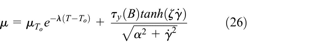
where
A one-way coupled model of an MR damper was presented by Parlak and Engin (2012) and Parlak et al. (2012), in which a steady-state magnetic solution was implemented by ANSYS/Magnetostatic, whereas the transient fluid flow analysis was implemented using ANSYS/CFX. The coupling strategy between the solvers is defined by the Bingham bi-viscous model, equation (10), using the CFX Command Language (CCL) used to define the coupling sub-routines in ANSYS/CFX. The same CCL method was used by Gurubasavaraju et al. (2018a, 2018b) to couple the fluid flow analysis implemented by ANSYS/CFX with the magnetic solution obtained by finite-element method magnetics (FEMM) software. The moving mesh technique which is important to define the piston motion is defined in ANSYS/CFX by the Command Expression Language (CEL).
Another coupling strategy was recently shown by Elsaady et al. (2020) using a user-defined function (UDF). UDFs are functions written in C++ which can be interpreted or compiled by ANSYS/Fluent CFD solver to improve its solution capabilities (ANSYS, 2011). For instance, a UDF can be used to customise boundary conditions, material properties, and source terms to the governing equations. Therefore, UDFs can dramatically upgrade the level of a CFD simulation to include different variables that are not included in the built-in library of the software, which is also the same in CCL and CEL employed in ANSYS/CFX. In Elsaady et al.’s (2020) study, the UDF was written to predefine the MR fluid viscosity in ANSYS/Fluent according to magnetic field density calculated by an FE model using COMSOL/Multiphysics, and the local shear rate generated in the CFD domain. The UDF was also used to define the piston motion and a variable time step for the CFD simulation.
Singh et al. (2014) developed a design optimisation technique for an MR damper using an FE model developed using ANSYS/APDL. The objective function was to maintain the maximum force of the damper below the value of 15 kN and to achieve the maximum velocity of the piston. A steady-state CFD analysis using ANSYS/Fluent CFD solver was developed in order to determine the viscous force of the damper. The flow was assumed to be Newtonian, as it was investigated in the absence of magnetic field. The pressure difference before and after the piston was calculated via the CFD analysis in order to be used to determine the overall damper force using an analytical model. Therefore, the approach presented by Singh et al. (2014) is a decoupled approach.
4.2.3. Predictions of the rheological behaviour of MR fluids (velocity and shear rate)
A 2D two-way coupled model of an MR damper using COMSOL/Multiphysics was presented by Case et al. (2013, 2014). The model is shown to predict the rheological behaviour of MR fluids in the activated and deactivated modes of the fluid to a very good degree of accuracy, as shown in Figure 11. The figure shows the contours of fluid shear rate in the MR damper when the piston is activated by an input current of 0.5 A, as shown in Figure 11(a), and in the deactivated mode, as shown in Figure 11(b). The figures are shown at time
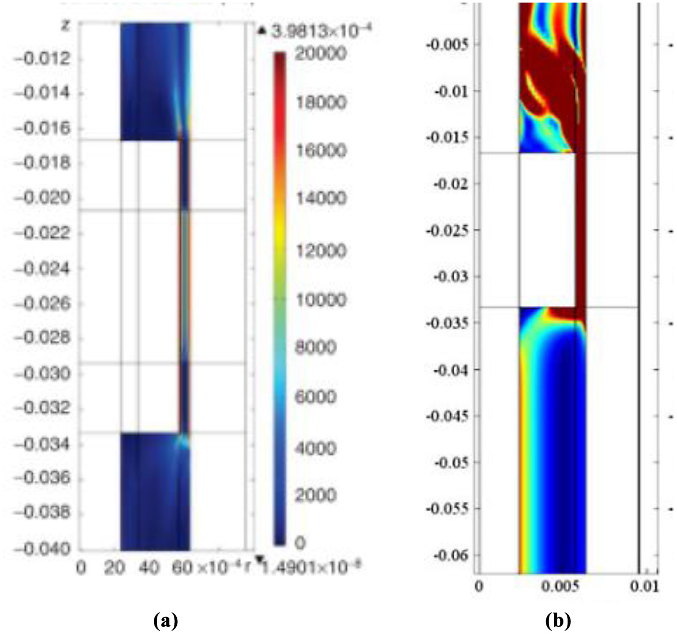
Predictions of shear rate contours of MR fluid inside an MR damper subjected to cyclic loads presented by Case et al. (2013, 2014): (a) when the fluid is activated by magnetic field at 0.5 A (Case et al., 2013) and (b) in the absence of magnetic field (Case et al., 2014).
Moreover, it can be seen in Figure 11(a) that the shear rate is so small at the farthermost ends of the piston (location of magnetic poles), whereas it is relatively higher in the middle region. This is because the magnetic field mainly flows from the magnetic poles causing the MR fluid in the farthermost ends of the piston to be more plugged than that in the middle region. Thus, the pre-yield region of the fluid located in the farthermost ends of the piston is relatively thicker.
In Figure 11(b) that was presented for the same damper in another research paper by Case et al. (2014), it is shown that the maximum shear rate exists in the throttling area which indicates that the velocity profile in the throttling area is nearly a fully developed Newtonian flow.
The variation of velocity profile along the throttling area of an MR damper was predicted by the CFD model presented by Parlak et al. (2012) using ANSYS/CFX. In that paper, the apparent viscosity of the fluid was defined in ANSYS/CFX for the MR fluid regions located at the farthermost ends of the piston. Therefore, the fluid streamlines, shown in Figure 12, in which the colours of the contours indicate the value of fluid velocity along the streamline, infer that the velocity profile changes along the throttling area of the MR damper due to the activated zones by magnetic field. This also matches the results obtained by Case et al. (2013, 2014), in which the results were shown by the shear rate contours.
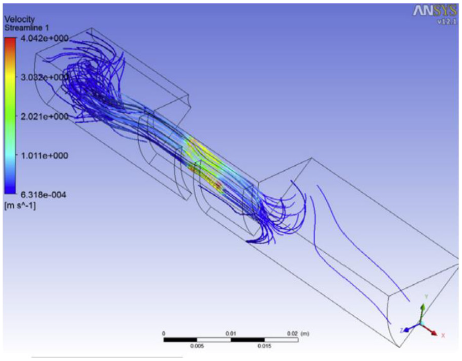
Fluid streamlines in an MR damper during compression stroke shown by Parlak et al. (2012). The contours indicate the value of fluid velocity along the streamline.
The analysis of the rheological behaviour of MR fluids in twin-tube MR dampers was also presented by Elsaady et al. (2020). The velocity profile in the throttling area of the damper shows the Couette–Poiseuille flow in the damper, as shown in Figure 13. The velocity profile is thought to be more realistic compared to the analytical 1D analysis presented in Figure 2(a), as it predicts the Couette flow caused by the motion of the piston in the left direction which causes a tiny portion of the fluid to move the same way according to the non-slip condition at walls (shear mode). However, the main flow is Poiseuille flow in the right direction due to the pressure difference along the annulus (flow mode). Moreover, although the pre-yield and post-yield regions can be observed, the interfaces between the regions cannot be clearly identified, which causes the velocity profile to be more realistic.
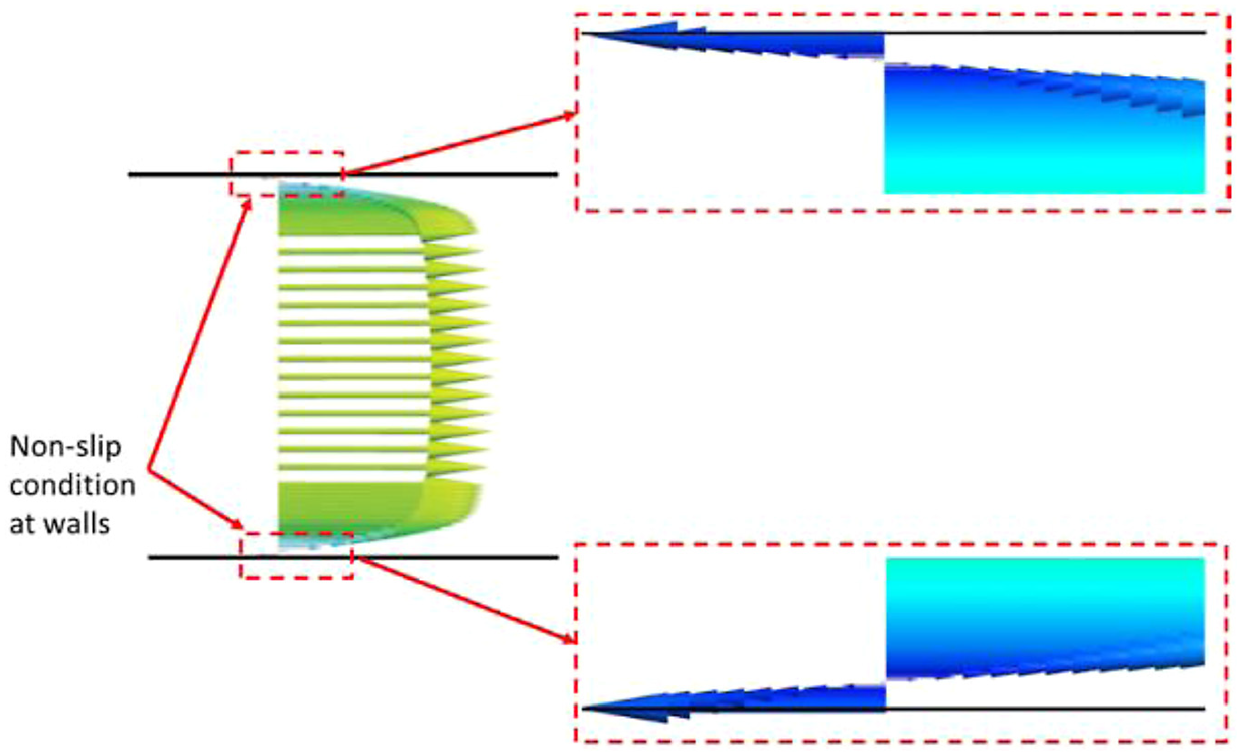
Velocity profile of the MR fluid in the throttling area of a twin-tube MR damper presented by Elsaady et al. (2020).
4.2.4. Predictions of apparent viscosity in numerical fluid flow models
The apparent viscosity of MR fluids is thought to be the most important parameter that should be predicted by numerical models, as it represents the coupled design parameter between different physics manifested by MR fluids. However, according to the literature available to the authors, the predictions of apparent viscosity of MR fluids in MR dampers were only seen in studies of Elsaady et al. (2020), Kemerli et al. (2019) and Parlak et al. (2012). The non-magnetised fluid zones which are not affected by magnetic field and the magnetised zones affected by magnetic field were presented, as shown in Figure 14(a) and (b). Figure 14(a) shows the viscosity contours presented by Parlak et al. (2012), whereas Figure 14(b) shows the contours presented by Elsaady et al. (2020). In both figures, the maximum value of the apparent viscosity are seen at the farthermost ends of the piston. However, the rheological behaviour is clearer to be inferred from the viscosity contours shown in Figure 14(b) compared to Figure 14(a). That is because the viscosity contours are shown to be low near the edges of the throttling area in Figure 14(b) where the shear rate is expected to be high, whereas that rheological behaviour is not clear in Figure 14(a). The reason for that is thought to be due to the very low number of nodes employed in the 3D mesh used by Parlak et al. (2012), as the mesh is composed of 6200 nodes which represents a 45° sector of the natural domain of the damper. The employed number of cells in the mesh used by Elsaady et al. (2020) is approximately 141,000 cells that only represent a 2D axisymmetric domain. A grid sensitivity analysis was shown in Elsaady et al.’s (2020) study, whereas it seems to be missing in Parlak et al.’s (2012) study.
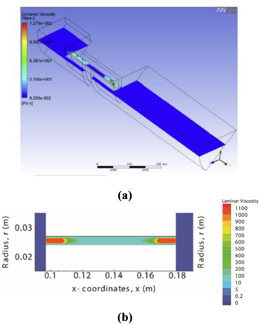
Predictions of apparent viscosity contours of MR fluids in MR dampers subjected to cyclic loads presented by Elsaady et al. (2020) and Parlak et al. (2012): (a) viscosity at
In order to verify that the low number of cells employed in the model presented by Parlak et al. (2012) is the main reason for misrepresenting the rheological behaviour in the viscosity contours, Kemerli et al. (2019) recently represented 2D models for the same MR damper investigated by Parlak et al. (2012). Kemerli et al. (2019) presented two models; one of them is coupled by using the same technique adopted by Parlak et al. (2012), whereas the other is a decoupled model. Although the recent study investigated a 2D domain, the number of cells was around 434,000, whereas the former study, in which a 3D model was presented, employed only 6200 cells. As a result, the viscosity contours by Kemerli et al. (2019) could predict the rheological characteristics of fluid viscosity following the same trend presented in Elsaady et al. (2020), as shown in Figure 15. It may be worth to note from the viscosity shown in Figures 14(b) and 15 that the convergence criteria can be analysed to be tighter by Elsaady et al. (2020) compared to those shown by Kemerli et al. (2019). This can be inferred from the smooth variations of contours shown in Figure 14(b), whereas the contours are more discretised in Figure 15.
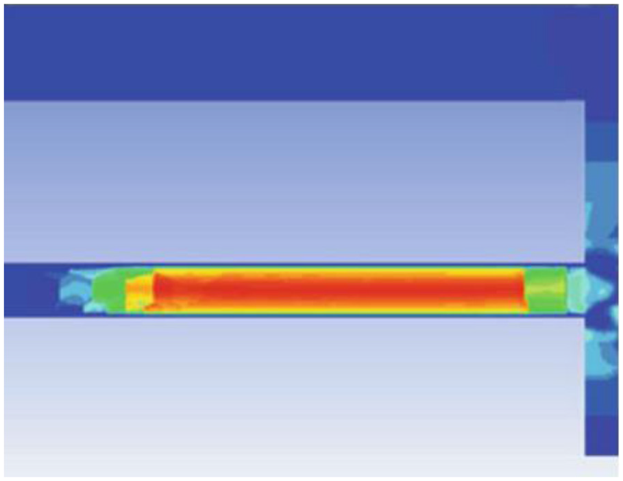
Predictions of apparent viscosity contours of MR fluids in MR dampers subjected to cyclic loads presented by Kemerli et al. (2019). The study was performed on the same damper presented by Parlak et al. (2012).
4.2.5. Analysis of nonlinear behaviour of MR dampers by numerical fluid flow solvers
Referring to the capabilities of numerical solvers illustrated in section ‘Advantages of numerical models within MR dampers’, they are expected to describe the nonlinear hysteretic behaviour of MR dampers to a better degree of accuracy. However, it seems that the numerical methods applied in the literature require more investigations on modelling the sources of hysteresis. The fluid inertia is accounted for according to the governing continuity and Navier–Stokes equations, shown by equations (21) and (22). However, other reasons for the hysteretic behaviour, namely, fluid compressibility, viscoelasticity, viscoplasticity and the presence of air/gas are not often accounted for in some of the studies presented.
In the time-dependent CFD model presented by Parlak and Engin (2012) and Parlak et al. (2012) using ANSYS/CFX, the model could not predict the hysteretic behaviour of the MR damper that was shown in experiments to the desired degree of accuracy. The authors attributed that misrepresentation of hysteretic behaviour to the handicaps involved in the deforming mesh technique. The same observation can be seen in other studies (Case et al., 2014; Singh et al., 2014; Zheng et al., 2014, 2015, 2017), in which only the work diagrams were used to validate the models developed. In the study by Zheng et al. (2014), where a coupled electromagnetic, thermal and fluid flow approach is presented, the performance of the damper was investigated at high piston velocity of 2 m/s and high amplitude of 0.34 m. It is believed that the hysteretic behaviour of the damper should be more remarkable under such high loads (Kim et al., 2015). However, the hysteretic behaviour was not shown in the results presented by Zheng et al. (2014), which can be inferred from the instantaneous transition of force at maximum displacements in the work diagram, as shown in Figure 16. The work diagrams are presented due to different combinations of the number of active coils.
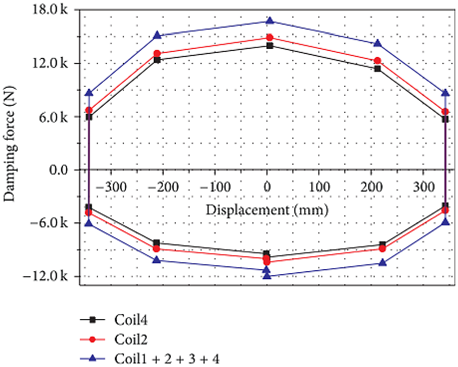
Work diagrams predicted by the two-way coupled numerical approach presented by Zheng et al. (2014).
It is thought that the main reason for the misrepresentation of the hysteretic behaviour by Case et al. (2014), Parlak and Engin (2012), Parlak et al. (2012), Singh et al. (2014) and Zheng et al. (2014, 2015, 2017) is due to the non-inclusion of compressibility, presence of air and viscoelastic effects in the fluid flow models. It has been shown by Elsaady et al. (2020) that the compressibility effects due to the presence of air mainly produce the hysteretic behaviour in twin-tube MR dampers. The effect of fluid inertia in producing the hysteretic behaviour was shown to be minor. That was due to the low values adopted for the motion conditions of the piston in terms of frequency and amplitude. The small contribution of fluid inertia to the hysteretic behaviour compared to compressibility was seen in Elsaady et al.’s (2020) study, as both effects were evaluated separately. The effect of fluid inertia is more remarkable when MR dampers are operated at high-frequency loads (Syrakos et al., 2016).
The hysteretic behaviour of MR dampers was also modelled and predicted by Guo and Xie (2019), in which the compressibility and viscoelastic effects were accounted for in a non-coupled CFD model, conducted with COMSOL/Multiphysics. The authors adopted a mono-tube MR damper with double-ended piston, which is a particular construction that eliminates possible presence of gas due to immersed/protruded part of the piston rod. The compressibility effects were defined in COMSOL/Multiphysics as a source term tensor in the Navier–Stokes equations applied in the model. A mathematical expression for each term of that source tensor was derived in order to express compressibility and viscoelastic effects. However, the variation of fluid density caused by the inclusion of that source tensor is only accounted in the Navier–Stokes equations, whereas the continuity equation assumes incompressible flow. Moreover, a constant distribution of magnetic flux in the damper throttling area was assumed in the model. This may imply that the proposed model by Guo and Xie (2019) overestimates the damper force, unless a weighted-average value of the yield stress over the throttling area was used.
In order to overcome the preceding two limitations of the model proposed by Guo and Xie (2019), the same authors (Guo and Xie, 2019) cooperated with others to present another FE model built with the general-purpose FEM solver in COMSOL/Multiphysics (Guo et al., 2019). In that model, the continuity and the momentum equations were developed in the weak form, and the effects of fluid inertia, compressibility, elasticity and friction were modelled in the equations. Also, the non-Newtonian viscosity was assigned only to the fluid regions adjacent to the magnetic poles of piston, as shown in Figure 17. Another in-house FV model was also developed for a mono-tube MR damper with double-ended piston by Syrakos et al. (2016). The model assumed incompressible flow. Therefore, the hysteretic behaviour of the damper was not predicted in the characteristic diagrams presented.
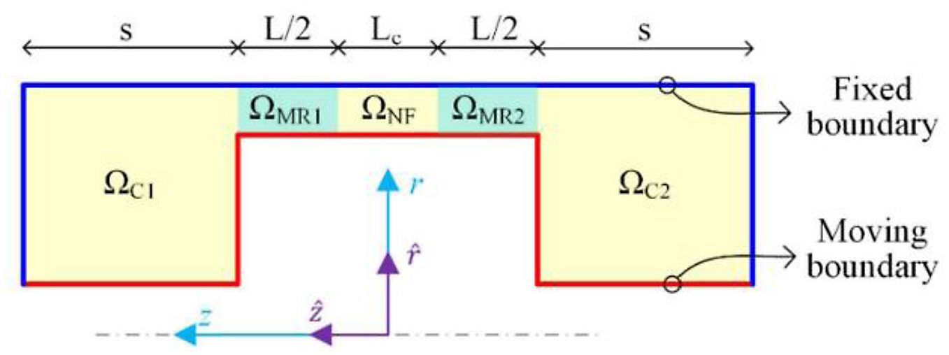
Fluid domains and boundary conditions of the FE model presented by Guo et al. (2019).
Although the CFD models presented by Kemerli et al. (2019) could predict the rheological behaviour of the MR fluid, as shown from the viscosity contours in Figure 15. Both the coupled and decoupled models were unable to predict the hysteretic behaviour of the damper that was shown in the experimental characteristics, as shown in Figure 18. The authors attributed that misrepresentation of hysteretic behaviour to the adopted assumptions in the CFD model. The work and characteristic diagrams according to the coupled and decoupled models are presented in Figure 18(a) and (b), respectively, in comparison with the experimental measurements. It is seen that both models depict the limiting values of the damper force to an acceptable degree of accuracy. However, the hysteretic behaviour was not predicted. The same results were also presented by Kemerli et al. (2018). It can be also inferred from Figure 18 that work diagrams are insufficient to assess the hysteretic behaviour of MR dampers, as it can be seen in Figure 18(a) that all curves are almost identical, except for the slight gradient of the experimental work diagram at the maximum values of piston displacement. However, these slight gradients cause a considerable difference in the characteristic diagram, as shown in Figure 18(b).
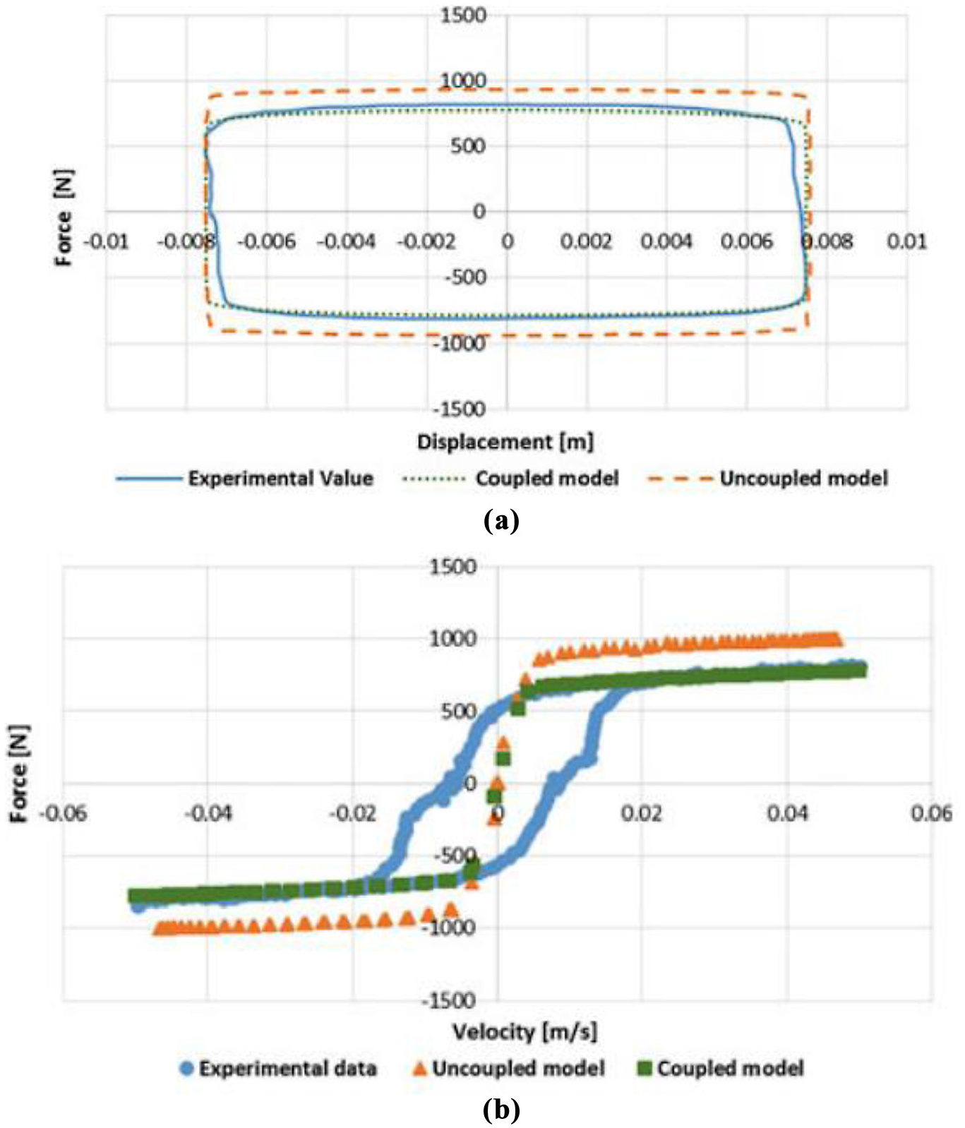
Work and characteristic diagrams according to the coupled and decoupled models presented by Kemerli et al. (2019), in comparison with the experimental measurements: (a) this model is coupled by the same technique adopted by Parlak et al. (2012), (b) this is a decoupled model.
To assert that the main reason for the misrepresentation of hysteretic behaviour in the aforementioned studies is the non-inclusion of the compressibility effects, two CFD models were developed by Elsaady et al. (2020); one of them assumes a single-phase incompressible flow; therefore, it only accounts for the effect of fluid inertia, whereas the other is a two-phase flow model that accounts for the effects of fluid compressibility and the presence of an air pocket in the damper. The single-phase incompressible CFD model was shown to misrepresent the hysteretic behaviour of the MR damper that was shown in the experimental characteristics, whereas the two-phase compressible CFD model predicts that behaviour, as shown in Figure 19.
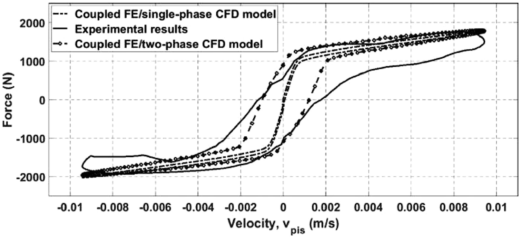
Characteristic diagrams according to the theoretical results of the single- and two-phase flow CFD models in comparison with experimental measurements presented by Elsaady et al. (2020).
It is worth mentioning that apart from the phenomenological reasons for the hysteretic behaviour of MR dampers, namely, magnetic hysteresis, fluid compressibility, inertia, viscoelasticity and the presence of air/gas in frequent designs of MR dampers, there is an original reason for that behaviour, which is due to the hysteresis mechanism in MR fluids themselves (Bai and Chen, 2019; Chen et al., 2017). In other words, there is a hysteresis mechanism during the flow of MR fluids, which is due to the energy required to dislocate the chains of ferromagnetic particles formed parallel to the magnetic flux lines. This hysteresis mechanism is often studied by microscopic models rather than macroscopic ones, as presented by Bai and Chen (2019), Chen et al. (2017) and Guo et al. (2014). Microscopic models investigate the equations of motion of ferromagnetic particles moving in single/multiple chains of dipoles in the MR fluid. Guo et al. (2014) developed a model that predicts the flow characteristics of MR fluids in shear mode. The model was validated by determination of the yield stresses of well-known types of MR fluids based on the model, and comparing the theoretical results with others due to experimental and referenced data. Bai and Chen (2019) developed a dipole model that could predict the hysteretic behaviour of an MR damper. They investigated the dynamic characteristics of a double-ended piston MR damper under very small conditions of piston excitations. They adopted that construction and those creeping motion conditions in order to solely evaluate the hysteresis mechanism of the MR fluid rather than those caused by fluid compressibility and inertia. A considerable hysteretic behaviour of the damper was found in the experiments conducted. They assumed that this hysteretic behaviour is entirely due to the hysteresis mechanism exerted by the fluid. Therefore, they developed a dipole model for single- and multi-chain structures of MR fluid flow in shear mode, and determined the yield strain of the fluid. The yield strain was found to be independent of the magnetic field strength or excitation current. Rather, it depends on the restoring force induced by the deformation of chains. Chen et al. (2017) developed a dipole model of the hysteresis mechanism exerted by MR fluids in valve and squeeze modes, in which the normalised restoring force was compared with that due to the shear mode.
5. Numerical approaches applied for MR applications other than MR dampers
The governing equations used for the modelling magnetic field and fluid flow phenomena in different MR applications are the same Maxwell’s, continuity, and Navier–Stokes equations presented in sections ‘Governing equations of magnetic field’ and ‘Improvements of numerical analysis of magnetic circuits of MR dampers’, respectively. Also, the same advantages and challenges reported to the use of numerical methods in MR dampers are applicable in many other MR fluid devices.
The procedure of modelling of magnetic field in different MR applications is similar to those applied for MR dampers. On the other hand, modelling of the fluid flow is thought to be more diverse according to the different design characteristics, assumptions, boundary conditions, and phenomena in each MR device. Therefore, the models may be applied to many types of domains, such as closed or open domains, single- or two-phase domain, stationary, rotating or moving domains.
In the following, some numerical approaches applied to MR fluid applications other than MR dampers are reviewed. The review of the articles in this section focuses on the methods applied, the software used and the parameters of interest. It can be analysed from the literature available to the authors that the numerical approaches applied to other MR applications are quite rare compared to those applied to MR dampers. The rareness of these studies is thought to be due to the difficulty and complexity of modelling the dynamic rheological behaviour of MR fluid, which is necessary to be modelled in these devices unlike MR dampers, in which there are alternative models which are based on nonlinear mechanics, as presented in section ‘Features of analytical parametric modelling of MR dampers’. These models can predict the performance of MR dampers without the complexity of investigating the flow characteristics of the fluid.
Therefore, more studies are required for MR applications other than MR dampers in order to predict their nonlinear performance. The available studies focus on understanding the general rheological behaviour of MR fluids in different cross-sections as will be illustrated in section ‘Flow of viscoplastic fluids in different cross sections’. Then, some research papers that study flow of MR fluids in squeeze and pinch modes are presented in section ‘Flow of MR fluids in squeeze and pinch mode’. The flow characteristics of these particular modes are thought to be not fully predicted compared to flow and shear modes, and that is why the available studies on these modes are grouped in section ‘Flow of MR fluids in squeeze and pinch mode’. Finally, some previous that presented numerical methods of different MR fluid applications are presented in section ‘Numerical approaches applied to different MR applications’.
5.1. Flow of viscoplastic fluids in different cross-sections
Cantelli (2009) developed a numerical viscoplastic model for the flow of viscoplastic fluids in ducts with rectangular, trapezoidal and triangular cross-sections. He introduced his findings by charts that define a dimensionless coefficient
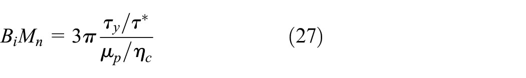
where
Common non-dimensional parameters used in MR fluid research, presented by Sherman (2016).
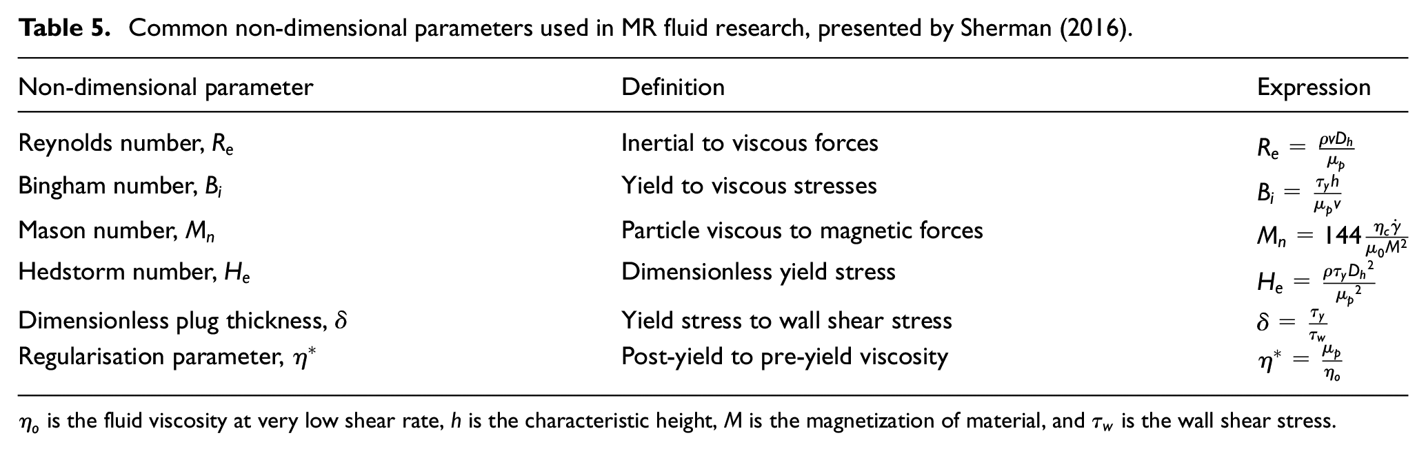
In rectangular cross-sections, Sherman (2016) developed correction factors for pressure difference exhibited by high-speed flows in rectangular ducts. The study accounts for inertial and friction effects. He applied CFD simulations using an FV analysis employed with OpenFOAM, and presented the results in the form of tables that presents the correction factors obtained from the CFD simulations. The simulations were performed for varying values of four parameters, namely, the hydraulic diameter,
Gedik et al. (2012) investigated the laminar flow of MR fluids between parallel plates, using ANSYS/Fluent Magneto-Hydrodynamics (MHD) module. Fluent/MHD module provides an environment to investigate the interaction between an applied electromagnetic field and a flow of an electrically conductive fluid (ANSYS, 2009). The magnetic field was applied perpendicularly to the direction of fluid flow in a small section of the parallel plates. Therefore, the velocity and pressure distributions were predicted by the developed steady-state CFD model. The higher pressure before the activated region by magnetic field was predicted, and the velocity profiles at different locations show the rheological properties of the fluid in the same manner presented in Figure 13. The velocity profiles were shown to be affected by magnetic field and the inlet velocity of the fluid. A recent study that also investigates flow of MR fluids between parallel plates was presented by Llorente and Pascau (2019), in which an in-house numerical code was developed. The results were validated with the counterparts obtained by Gedik et al. (2012), in which the Fluent/MHD module was used.
Omidbeygi and Hashemabadi (2013) investigated the flow of MR fluids in an eccentric annulus using analytical and numerical methods. The annulus is composed of two parts; an inner part that rotates with a certain angular velocity and a stationary outer part. The predictions of tangential velocity, torque and pressure gradient according to the analytical model were compared with those due to a 2D numerical model developed using FEMLAB/Multiphysics. FEMLAB is the former name of COMSOL/Multiphysics. Therefore, the presented numerical model in that study couples the electromagnetic and fluid flow solvers in the same two-way scheme illustrated earlier for COMSOL/Multiphysics in section ‘Coupling between magnetic and fluid flow solvers’. Another study for the flow of MR fluids in a concentric annulus was presented by Damianou et al. (2019), in which the flow was modelled analytically.
5.2. Flow of MR fluids in squeeze and pinch modes
Research on flow of MR fluids in squeeze and pinch modes, described by Figure 2(c) and (d), respectively, is quite rare (Sapinski and Gołdasz, 2018). The flow characteristics of these modes are thought to be not fully predicted (Gołdasz and Sapiński, 2015a; Gołdasz et al., 2018). Employment of squeeze mode in MR fluid devices, either being standalone or merged with the shear mode is found to conduce higher performance of MR devices (Farjoud et al., 2011; Lee et al., 2019; Wang et al., 2019). Pinch mode is also a recent mode that attracts more interest in some MR fluid devices (Lee et al., 2019; Tao, 2019). Hereinafter, some pieces of research on those modes are analysed.
5.2.1. Flow of MR fluids in squeeze mode
Gstöttenbauer et al. (2008) presented a numerical model of the stress and deformation of MR fluids in squeeze mode. They applied an FE model using ABACUS software, in which the MR fluid was placed between two parallel discs and a sinusoidal motion was applied to the upper disc. The von Mises equivalent stress was determined by the model, and it was found to be dependent on the hydrostatic pressure.
Farjoud et al. (2011) presented a semi-analytical model of flow of MR fluids in squeeze mode. The velocity field, the distribution of pressure and shear rate, and the total squeeze force were determined via a quasi-static 2D model. The Bingham–Papanastasiou model defined by equation (4) was used to define the fluid viscosity. Also, Farjoud et al. (2009) developed a non-dimensional model validated by experiments for a rheometer operated in squeeze-mode.
Gołdasz and Sapiński (2015a) developed a CFD model of an MR damper operated in squeeze mode. The model couples the effect of variable magnetic field that leads to the variation of fluid yield stress in the fluid domain. They developed the model using ANSYS/Fluent software in which the fluid viscosity was defined by the Bingham bi-viscous model defined by equation (10). The dynamic characteristics of the damper force were determined based on the numerical CFD model and another analytical model. The same authors collaborated with Rosół and Jastrzębski by Sapiński et al. (2017) to give insight into the characteristics of MR dampers operated in squeeze mode based on experimental measurements. A prototype of an MR damper with the same design presented by Gołdasz and Sapiński (2015a) was manufactured and tested. The study also included a comparison of the damper behaviour due to operation within open- and closed-loop control circuits. Moreover, a model for the magnetic circuit of the damper was developed by Sapiński and Gołdasz (2015).
Recently, Wang et al. (2019) designed a high-torque rotary MR damper with water cooling operated in squeeze and shear modes. The study presents an analytical model that determines heat generation and dissipation by the damper. The model was validated by the experimental measurement of the braking force at different temperatures. The experimental results indicate that operation of the rotary MR damper in the hybrid squeeze-shear mode implies high damping torque of the damper.
5.2.2. Flow of MR fluids in pinch mode
An MR fluid valve operated in pinch mode was patented by Carlson et al. (2008). The direction of magnetic flux in this mode is parallel to the direction of flow. Therefore, the fluid is throttled in an orifice controlled by magnetic field. Also, the fluid can be totally jammed up to a certain pressure if the magnetic field strength is high (Goncalves, 2009). Recently, operation of MR fluid devices in pinch mode has attracted more interest in other applications rather than MR valves. The pinch mode was proven to be effective for the purpose of suppressing turbulence of blood and crude oil flow, as shown by Du et al. (2018), Tao (2019) and Tao and Huang (2011).
Regarding numerical modelling of MR fluids in pinch mode, a magneto-static analysis was presented by Gołdasz and Sapiński (2017), whereas a fluid flow analysis was presented by Gołdasz et al. (2018). A magnetic FE model employed with a quasi-static analytical model was also introduced by Lee et al. (2019). In Gołdasz and Sapiński’s (2017) study, some magnetic circuits were designed and modelled using an FE model applied in FEMM software. The magnetic circuits employ different configurations using different number of coils and heights of flow gap. The results indicated that the flow rate of fluid can be effectively controlled by tuning the input current. On the other hand, a numerical CFD model of the pinch-mode flow of MR fluid between parallel plates was studied by Gołdasz et al. (2018). Steady-state incompressible flows with different conditions were simulated using ANSYS/Fluent software. Different cases that adopt different Reynolds numbers
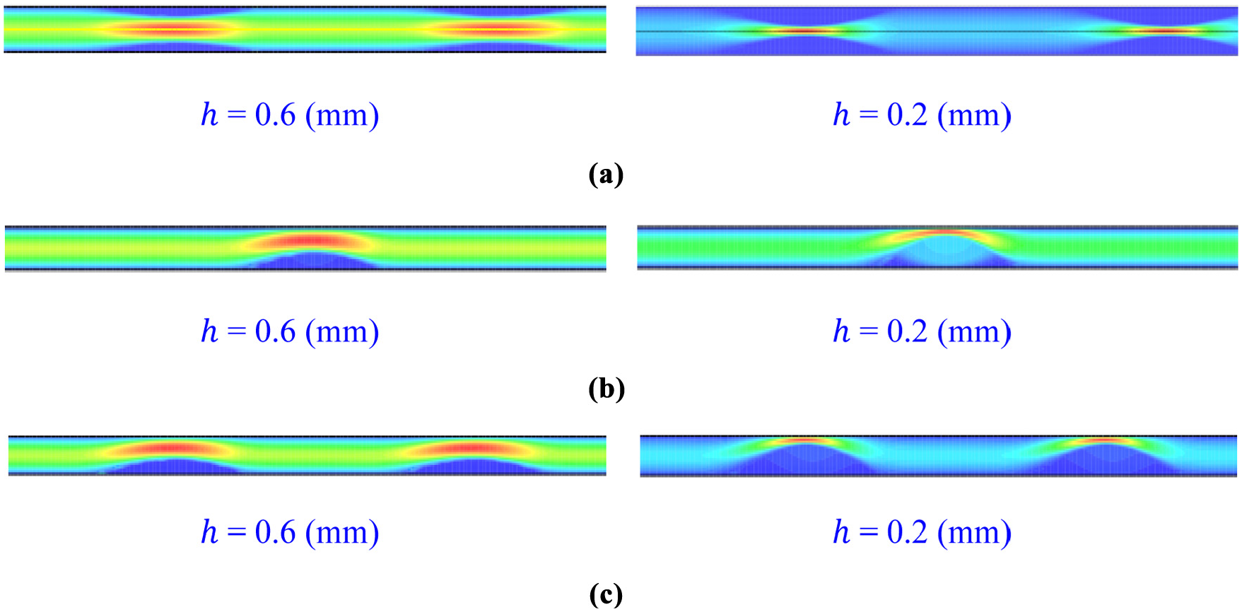
Theoretical velocity contours of the flow of MR fluid in pinch mode between two parallel plates (
5.3. Numerical approaches applied to different MR applications
5.3.1. MR clutches
Ellam et al. (2006) investigated the Couette flow of MR fluids between parallel plates and in concentric annuli. They developed an analytical model for the flow in parallel plates, and another steady-state, incompressible and isothermal CFD model for the flow in concentric annuli using ANSYS/Fluent. The constitutive equation of viscosity was defined by a UDF to the CFD model using the bi-viscous Bingham model, defined by equation (10). The authors used their results to analyse the flow in concentric and radial MR clutches. Different models of the clutches were proposed in which analytical and CFD solutions were developed. It was shown that the analytical parallel-plate assumption is valid as an approximation to the CFD annular model.
Later CFD models were developed by the first and third authors of the preceding study, who collaborated with Wong and Tozer in a study by Bullough et al. (2008). The authors aimed to give insights into modelling and simulation of different smart ER/MR devices, which is useful for the guidance of design and pre-prototyping stage of these devices. Therefore, they presented similar CFD models to the preceding study for 1D and 2D flow in MR clutches, MR valves and piezoelectric poppet valve. The study shows the predictions of the effects of different design parameters that cannot be determined by analytical models and were attained by the CFD models, namely, the effects of friction, inertia and heat generation were predicted.
5.3.2. MR valves
Wang et al. (2009a) designed, modelled, fabricated and tested an MR valve with annular and radial MR regions operated in valve mode. An FE model of the magnetic circuit in the valve was developed using ANSYS/Emag and solved in conjunction with an analytical solution of the fluid flow. It was shown that the use of radial MR regions leads to a higher pressure drop, and consequently a higher efficiency of the MR valve. Moreover, the use of radial and annular MR regions leads to better controllability of the performance of the MR valve. The results of pressure drop at different input currents were validated by experimental measurements, in which the maximum difference between theoretical and experimental results is around 25%. Operation of MR valves in pinch mode rather than flow mode was proven to be advantageous as presented in section ‘Flow of MR fluids in squeeze and pinch modes’, as it allows the increase of pressure drop in the valve regardless of the velocity of fluid flow (Lee et al., 2019).
5.3.3. MR journal bearing
Bompos and Nikolakopoulos (2011) presented a one-way coupled numerical approach to model the performance of eccentric MR journal bearings. The approach combines an FE model developed using ANSYS/APDL of magnetic circuit analysis and a steady-state CFD model applied with ANSYS/Flotran of fluid flow analysis. They presented an insight into the effects of different design parameters of journal bearings, namely, eccentricity, attitude angle between the line passing through both centres of the eccentric journal and bearing and the vertical axis, oil flow rate and friction coefficients of the journal and bearing surfaces. Recently, Sahu and Sharma (2019) developed an FE model for eccentric MR journal bearings implemented using MATLAB. The model integrates analyses of fluid flow, lubricant flow and temperature effects. They validated their work with published work according to different design parameters.
5.3.4. MR prosthesis
A decoupled numerical approach was recently presented by El Wahed and Wang (2019). The flow of MR fluid in the gap of a ball-and-socket structure was investigated by numerical and experimental methods. The aim of that work was to develop an MR shoulder joint that helps in human shoulder rehabilitation. The magnetic field distribution in the flow gap was assumed to be constant, and the built-in Herschel–Bulkley model in ANSYS/Fluent software was used to determine the resistive torque exerted by the fluid due to the angular motion of the ball. The sliding mesh technique available in ANSYS/Fluent was used to simulate the rotary motion of the ball. Another theoretical model based on Bingham plastic model was developed. However, the numerical model was found to predict the damping torque of the ball-and-socket more accurately than the analytical model in comparison with the experimental results.
5.3.5. MR rotary dampers
Li et al. (2019b) presented a transient two-way coupled model of a rotary MR damper using COMSOL/Multiphysics. The constitutive equation employed for the viscosity definition was the hyperbolic tangent function defined by equations (9). The equation was modified to include the effect of fluid temperature in the model. The model accounts for four studies, namely, magnetic field, fluid flow, heat transfer and structural mechanics, in which the thermal stresses were accounted for. The first three studies are implemented in a two-way coupled model, whereas, the structural mechanics study is implemented by a one-way technique, in which the load is imported from the fluid pressure and temperature determined by the fluid flow and heat transfer studies. The results of the distributions of magnetic field, temperature, thermal and total stresses are shown. The results were verified by the experimental measurements of the braking torque, braking time and surface temperature of the damper at different locations at the end of braking. The results show fairly good accuracy between the computational and experimental data. It can be seen from that study the advantages of applying coupled numerical models in the multi-physics analysis of MR fluid devices in order to study the interacting phenomena occurring in these devices. The augmentation of squeeze mode with the shear was shown to enhance the performance of rotary dampers, as presented by Wang et al. (2019).
5.3.6. MR fluid stirring device
One of the most recent MR fluid devices that has been investigated by a numerical CFD technique is and MR fluid stirring device, as presented by Tian et al. (2020). The objective of that study was to optimise the mixing time of MR fluid ingredients with the aid of CFD modelling. Therefore, an ordinary mixing device was modelled using the multiple reference frame (MRF) and the Euler mixture models employed in ANSYS/Fluent. The MRF model is a steady-state model, in which rotational and/or translational movements can be assigned to some of domain zones (ANSYS, 2011). Then, another mixer was modelled, then the dimensions and rotating velocity of the mixer were optimised to achieve the least mixing time. The simulations were performed with different geometries and number of the baffles in order to achieve the fastest homogeneous distribution of solid particles in the mixer. Finally, the mixer with the optimised dimensions was manufactured and tested. The reduction in mixing time due to the optimised mixture was found to be 83% less relative to that of the traditional mixer. However, it is thought that more considerations should be accounted for in the preceding study, such as the effects of buoyancy and surface tension of the fluid. Moreover, the CFD simulations were performed in a very short-time interval, in which the homogeneous distribution of solid particles was achieved. However, the consistent homogeneity of the fluid over a longer time interval was not investigated, which is thought to be so hard to be studied by numerical models.
6. Conclusion
The aim of this article was to review the state-of-the-art numerical models applied to MR fluid devices and applications for the first time in the literature. It has been shown that the use of MR fluids in different MR applications is continuously growing, which increases the necessity for better understanding of the flow characteristics. However, most of the analytical methods applied in MR fluid research may be insufficient to predict the characteristics of MR fluids. That is because most analytical models, despite being able to evaluate the dynamic characteristics of some MR fluid devices, may not give an insight into the rheological fluid flow behaviour. That behaviour is affected by several phenomena that may not be accounted for in analytical models, such as transient, inertial and compressibility effects, presence of air as a pocket or air bubbles in the fluid and possible cavitation and turbulence.
The implementation of numerical methods in MR fluid research has been shown to be more advantageous in comparison with analytical models. The numerical methods can account for more phenomena and design parameters and be subject to fewer assumptions compared to analytical models. However, numerical models of MR devices are more difficult and complicated. The challenges encountered in modelling and simulation of an MR device and research efforts towards overcoming these challenges have been discussed, namely, (1) the need to implement coupling between magnetic and fluid flow solvers, (2) the need to develop viscoplastic relations in numerical approaches other than those used in analytical models, (3) the need to assign the magnetic effect to a part of the fluid domain in the fluid flow solver, and (4) the need to develop a transient simulation that may involve a moving mesh technique in the fluid flow solver.
The reviewed research papers that investigate numerical approaches for MR applications show that the methods of numerical modelling and simulation of magnetic field are quite consistent and achievable. However, the methods of numerical modelling and simulation of flow field are diverse and they vary between FE- and FV-based methods. There is no clear assessment on the suitability of different methods in MR fluid device research in terms of accurate predictions of different phenomena, numerical stability, applied models and computational cost.
The reviewed literature that investigate numerical approaches of MR dampers show that the methods applied in different research papers are seen to complement one another. Different solvers that apply FE- and FV-based methods for investigation of fluid flow are seen in one- and two-way coupled approaches. However, not all the reviewed papers are found to fully predict the flow parameters such as velocity profile, viscosity, shear rate, and hysteretic behaviour. Nevertheless, the limiting dynamic force magnitudes were predicted fairly accurately. The predictions of velocity, viscosity and shear rate profiles were seen in few research papers. Moreover, the accurate prediction of the hysteretic behaviour of MR dampers using numerical approaches was only seen in Elsaady et al. (2020), Guo and Xie (2019) and Guo et al. (2019). The reason for that is due to the consideration of the effect of fluid compressibility and the presence of air in Elsaady et al.’s (2020) study, whereas the compressibility and viscoelastic effects were accounted for by Guo and Xie (2019) and Guo et al. (2019). The other pieces of literature available to the authors were found to misrepresent the hysteretic behaviour. The characteristics of the models applied in the available literature were reviewed.
It has been found that the reviewed literature that investigate numerical approaches employed in MR applications other than MR dampers are quite rare. The reason for that rareness is thought to be due to the complexity of modelling the rheological behaviour of MR fluids, which is necessary to be modelled in these devices unlike MR dampers. The available pieces of literature focus on predicting the flow characteristics of MR fluid in different cross-sections. Few research efforts were oriented to different MR applications such as MR valves, journal bearings, rotary dampers and clutches. However, the importance of the multi-physics analysis of MR fluid devices was shown by Li et al. (2019b), in which a model that couples studies for magnetic field, fluid flow, heat transfer, mechanical and thermal stresses was presented and verified by experimental measurements.
The presented review is thought to expand the understanding of the diversity of numerical methods applied in MR fluid device research, and also other research on devices that exhibits multi-physics phenomena. The methods presented in the literature whose characteristics are discussed in this article are thought to be useful for better assessment of the suitable numerical methods applied within MR fluid device research. The article may also give some guidance for future researches in which more phenomena and design parameters will be considered in order to predict the nonlinear behaviour of MR fluid devices.
Footnotes
Declaration of conflicting interests
The author(s) declared no potential conflicts of interest with respect to the research, authorship and/or publication of this article.
Funding
The author(s) received no financial support for the research, authorship and/or publication of this article.