
Abstract
Camber morphing aerofoils have the potential to significantly improve the efficiency of fixed and rotary wing aircraft by providing significant lift control authority to a wing, at a lower drag penalty than traditional plain flaps. A rapid, mesh-independent and two-dimensional analytical model of the fish bone active camber concept is presented. Existing structural models of this concept are one-dimensional and isotropic and therefore unable to capture either material anisotropy or spanwise variations in loading/deformation. The proposed model addresses these shortcomings by being able to analyse composite laminates and solve for static two-dimensional displacement fields. Kirchhoff–Love plate theory, along with the Rayleigh–Ritz method, are used to capture the complex and variable stiffness nature of the fish bone active camber concept in a single system of linear equations. Results show errors between 0.5% and 8% for static deflections under representative uniform pressure loadings and applied actuation moments (except when transverse shear exists), compared to finite element method. The robustness, mesh-independence and analytical nature of this model, combined with a modular, parameter-driven geometry definition, facilitate a fast and automated analysis of a wide range of fish bone active camber concept configurations. This analytical model is therefore a powerful tool for use in trade studies, fluid–structure interaction and design optimisation.
Keywords
Introduction
Due to the nature of aircraft flight operations, the lift coefficient required to sustain flight varies depending on the flight stage. Factors such as aircraft weight (variable during flight), altitude, atmospheric conditions and manoeuvres determine the required lift coefficient at a specific flight stage. There are currently two main approaches to generate these variations in lift coefficient: changing the angle of attack of the whole aircraft or by varying camber distribution. The latter approach can be achieved with traditional control surfaces and high lift devices (i.e. ailerons, elevator, trailing edge flaps), which consist of hinged panels attached to the central wing. Although the deflection of these hinged panels causes an effective variation in lift force, the sharp change in aerofoil section produces a significant drag penalty and noise. While the drag associated with manoeuvres does not typically make a significant impact on fuel burn over a mission, the significant drag penalty of traditional plain flaps makes them an unattractive option for more ambitious attempts to actively and continuously control the camber of the entire wing as a means of directly affecting the efficiency of the aircraft.
Camber morphing allows aerofoil properties to be modified with a much lower drag penalty, as the changes in camber occur in a smooth and continuous way. An ideal solution to this issue is to generate a smooth and continuous change in camber distribution. These not only make camber morphing devices attractive to replace trailing edge hinged plain flaps, but also to be actively used during flight to optimise the spanwise lift distribution.
As a consequence, there has been a significant motivation to develop wings that are capable of continuously adapting their geometries to different flight scenarios. These types of wings are known as morphing wings, and they are used as a method to improve the overall aerodynamic performance of aircraft. These research efforts are summarised by Thill et al. (2008), Barbarino et al. (2011) and Valasek (2012); specifically, all authors highlight that one of the most commonly pursued and researched method to optimise aerodynamic performance, at several flight stages, is active changes in the camber distribution of aerofoils.
One of the first designs that targeted variable camber without surface discontinuities was presented in the NASA’s F-111 Mission Adaptive Wing Aircraft, where a variable camber wing is implemented to optimise aerodynamic performance at different flight scenarios (Larson, 1986). Another variable camber concept is the DARPA Smart Wing (Kudva, 2004), where a centre laminate with honeycomb core and silicone skin give the trailing edge the flexibility needed to create changes in camber (Figure 1).
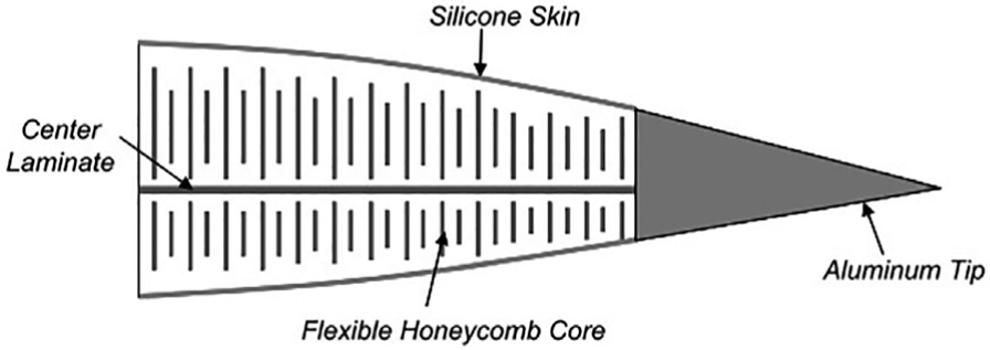
DARPA smart wing variable camber concept. Reproduced from Kudva (2004), with author’s permission.
Some research groups have studied variable camber using leading edge devices: Vasista et al. (2017) designed and manufactured a compliant ‘droop-nose’ morphing leading edge device using superelastic materials. Furthermore, combining leading and trailing edge morphing within the same wing has also been investigated: Kota et al. (2003) performed a study on the feasibility of variable camber combining both leading and trailing edge morphing devices using both voice coil motors and piezoelectric actuators, while De Gaspari et al. (2014) designed, manufactured and tested a variable camber wing with morphing leading and trailing edge devices based on compliant-based mechanisms. Also, Monner et al. (2009) proposed a composite monolithic compliant morphing trailing edge device; however, no actuation mechanism was selected. Moreover, De Gaspari and Ricci (2010) performed a two-level optimisation that first obtained the ‘best’ aerofoil configuration for a given condition, followed by obtaining the best internal structural configuration capable of achieving such aerofoil geometry.
Furthermore, other concepts achieved variable camber by focusing the camber changes on the trailing edge, for example, by embedding actuators within the wing skin (Bilgen et al., 2011; Molinari et al., 2011), exploiting bistability in non-symmetric fibre-reinforced composite laminates (Daynes et al., 2010; Diaconu et al., 2008) and also by active actuation of the internal load-bearing structural members (Barbarino et al., 2009; Grohmann et al., 2008; Milojević and Pavlović, 2016; Previtali et al., 2015).
One concept which has shown promise is the fish bone active camber (FishBAC), introduced by Woods and Friswell (2012). This compliance-based morphing aerofoil device consists of a biologically inspired internal skeletal structure covered with a flexible skin. The skeleton consists of a central bending beam spine with a series of stringers branching off to support the skin, which is made from pre-tensioned elastomeric materials (Figure 2). This structure is highly anisotropic by design, with a low chordwise bending stiffness but high spanwise bending stiffness. The resulting bending moments due to actuation loads then deform the structure in a manner, which produce smooth and continuous changes in camber distribution, with the highly anisotropic nature of the structure focusing the deformation on the desired camber shape.
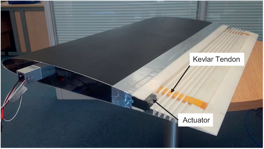
FishBAC morphing trailing edge concept (white), attached to a ‘rigid’ wing (black) and actuated by a pair of antagonist tendons (yellow).
Preliminary wind tunnel tests of this structural design show promising results in terms of lift control authority (
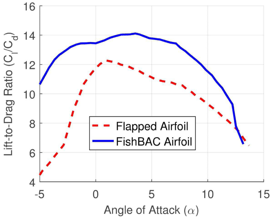
Lift-to-drag ratio versus angle of attack of the isotropic FishBAC. Experimentally obtained by wind tunnel testing (Woods et al., 2014).
However, it is precisely these variations in spanwise deformation that are of great interest as they can be exploited to also optimise the spanwise load distribution of the wing. The ability to have significant control over the spanwise distribution of lift on a three-dimensional (3D) wing would provide a number of potential induced drag, structural, control and aeroelastic benefits. The presented model addresses these shortcomings by modelling the FishBAC using a two-dimensional structural formulation based on Kirchhoff–Love plate theory. This approach is more suitable for the intended application as variations in out-of-plate displacement due to several factors, such as bend–twist coupling, differential actuation inputs and 3D aerodynamic effects (Anderson, 2010), can be captured and eventually be exploited to optimise lift distributions in both chord and spanwise directions. Also, another advantage of modelling the structure using plate theory is to exploit material anisotropy by including classical laminate theory (CLT) formulations within the plate’s differential equation. Derivations of the equations of motions and strain energy of composite laminated plates are well established (Whitney, 1987), and consequently, they can be implemented to design a composite FishBAC prototype.
The objective of this work is to develop an analytical model of the FishBAC concept that captures thein-plane and out-of-plane displacement due to both aerodynamic pressure (i.e. transverse loading distribution) and actuation loads (i.e. point moments at the trailing edge). This model is able to analyse the discontinuous geometry of the FishBAC by modelling its variable stiffness as multiple individual plates that are joined by penalty springs, capturing its complexity within a single system of linear equations. The scope of this work not only represents a more capable approach to modelling the FishBAC, but also shows an advance — beyond existing techniques in literature — in modelling complex discontinuous plate structures. Currently, there is evidence in the literature of neither the use of penalty springs to join a significant number of individual plate partitions (115 in this case) nor the use of Rayleigh–Ritz method to model static deflections under transverse pressure and line moments of such complex assembly.
The analytical nature of the model not only allows local stiffness properties to be defined for each individual plate ‘partition’, but also to rapidly modify the geometric parameters (e.g. stringer spacing, spine and skin thickness, wing dimensions, among others) and material properties. Finally, unlike finite element method (FEM), the analytical model is ‘mesh independent’, which means that its convergence only depends on the number of the assumed shape functions that are used.
This article is structured as follows: first, an introduction of the FishBAC morphing concept and the initial geometric modelling assumptions is presented, followed by a brief description of the Rayleigh–Ritz method, assumed shape functions, boundary conditions and model implementation. Finally, a convergence study and comparison with FEM results are introduced as a validation to the developed analytical model.
Structural configuration
As described by Woods and Friswell (2012), the FishBAC’s main load-bearing member is a central ‘spine’ that follows the aerofoil camber line. Attached to it, a series of perpendicular stringers of varying heights support the skin, maintain the aerofoil thickness distribution and also increase the spanwise stiffness of the whole structure. The height of the stringers decreases in accordance with the aerofoil geometry. A pre-tensioned elastomeric skin is attached to the stringers and acts as the aerodynamic surface of the FishBAC. Pre-tensioning the skin significantly reduces the out-of-plane deformations under aerodynamic loading and also prevents skin buckling, which would otherwise occur due to compressive strains induced by camber morphing.
The structure is actuated by a pair of antagonistic tendons each driven by independent actuators that are attached to the top and bottom of the trailing edge, respectively. The antagonist pair transfers the torque generated by the actuators, located at the root of the FishBAC, to the trailing edge of the aerofoil section (Figure 4). In the structural analysis, the actuation loads are modelled as applied moments at the tendon-solid trailing edge joints.
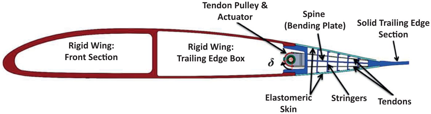
Schematic of the structural configuration of the fish bone active camber morphing trailing edge concept (Woods and Friswell, 2014).
Finally, the FishBAC trailing edge device integrates readily with the existing structural solution for the primary load-bearing member that carries the majority of the aerodynamic loads. While the cross-sectional geometry of the primary load-bearing spars may vary depending on the particular application (e.g. box section, D-spar, channel section), the FishBAC can be readily adapted to suit. Given its use with traditional high stiffness wing geometries, one of the initial assumptions is that the deflection in the primary spar is negligible, which is to say that a ‘rigid’ front portion of the wing is assumed in this initial portion of the work. As a consequence, the analytical model presented in this article only focuses on the deformation of the compliant morphing trailing edge section, which is assumed to be ‘clamped’ to this rigid front portion of the wing. Therefore, the FishBAC is modelled as a cantilever plate with three free edges. A detailed explanation of the modelling assumptions and boundary conditions is given in the next sections of this article.
Modelling assumptions: geometry and materials
The analytical model developed here assumes that the spine’s initial geometry (Figure 5(a)) is a flat plate with no initial curvature (Figure 5(b)). For symmetric aerofoils, this assumption has no effect, but for cambered aerofoils, it flattens out the small amount of curvature that exists in the camber line over the morphing region. Due to this initial assumption, a number of ‘simplifications’ are applied to the geometry, such as the skin is flat and parallel to the spine and each skin section is located at an equivalent height (from the spine) that is calculated by estimating the equivalent contribution in second moment of area of the curved skin in the original design. Finally, the solid trailing edge section is ‘discretised’ in five sections of constant thickness.
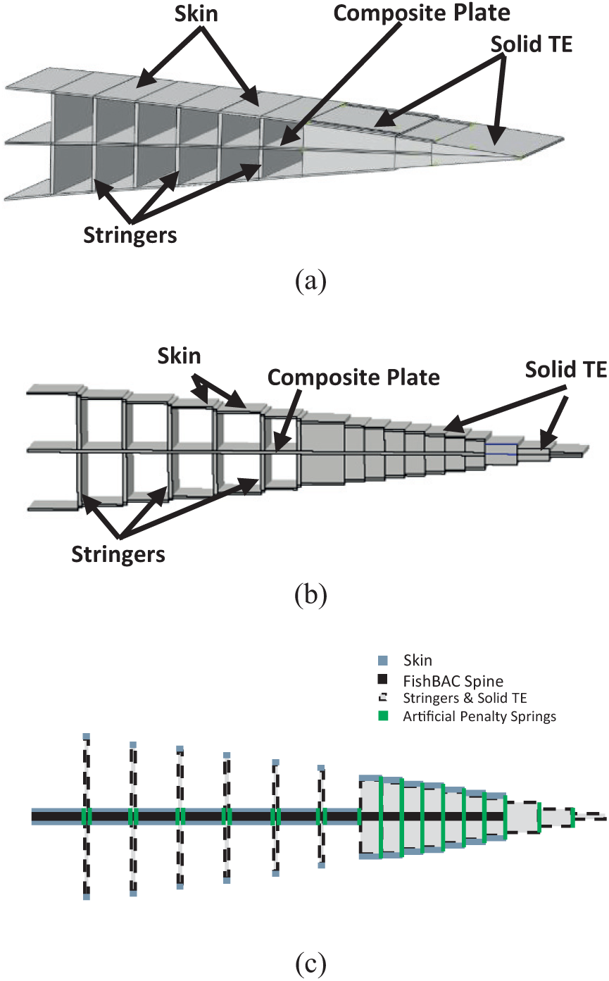
FishBAC’s geometry (a), simplified geometry (b) and modelling assumption (c). In the FishBAC geometry (a), the spine follows the camber line of the aerofoil section, while in the simplified geometry (b), the spine presents no curvature. Furthermore, the stiffness of each partition is ‘condensed’ at the local mid-plane, and each partition is joined using a series of artificial torsional springs (c).
Furthermore, in order to capture the significant stiffness discontinuities caused by the stringers, the structure is divided into several partitions of uniform thickness distribution and composite stacking sequence (chordwise and spanwise) and the plate’s energy balance is solved in each partition, individually. Each one of these individual ‘plates’ are then joined together by artificial torsional springs at each local boundary. This method is known as the Courant’s penalty method (Ilanko et al., 2015) and is explained in detail in the following sections of this article. Finally, the stiffness of each partition is ‘condensed’ at its mid-plane (Figure 5(c)) using CLT. This means that displacement and rotation compatibility is only enforced at the mid-plane and not at the stringers–skin joints. This assumption is reasonable and expected to be valid for the FishBAC due to the compliance of the skin. As the materials used for the stringers and spine are at least three orders of magnitudes stiffer than the elastomeric skin, there is no risk of structural penetration at the skin–stringer contacts if compatibility is not enforced at these locations.
Figure 5 shows a comparison between the FishBAC’s actual geometry (Figure 5(a)), the assumed geometry in the analytical model (Figure 5(b)) and the ‘condensed’ stiffness assumption at the mid-plane (Figure 5(c)). Note that the geometry of finite element model that is used to validate the analytical model corresponds to the actual geometry (Figure 5(a)), which allows to validate simultaneously the underlying geometry assumptions and the implementation of the methods. Further details about the FEM model and the validation process are discussed later.
For a model of the size of a Unmanned Aerial Vehicle (UAV) wing or helicopter rotor blade, three types of materials are used throughout this analysis: high-strength carbon fibre–reinforced polymer (CFRP), acrylonitrile butadiene styrene (ABS), 3D printed plastic and silicone rubber. The stringers and solid trailing edge sections are modelled using isotropic ABS plastic, while the skin is modelled as isotropic silicone. This material selection for stringers, solid trailing edge and skin was performed based on the materials that were used for manufacturing the isotropic FishBAC wind tunnel prototype (Woods and Friswell, 2014) and also because these also may be used to manufacture the first FishBAC composite prototype. Finally, the composite spine is modelled using high-strength CFRP. Table 1 presents the stiffness values of each one of the material definitions.
Material properties of CFRP (Datoo, 1991), ABS (Cambridge University Engineering Department (2003)– Materials Data Book) and silicone (Woods and Friswell, 2013).
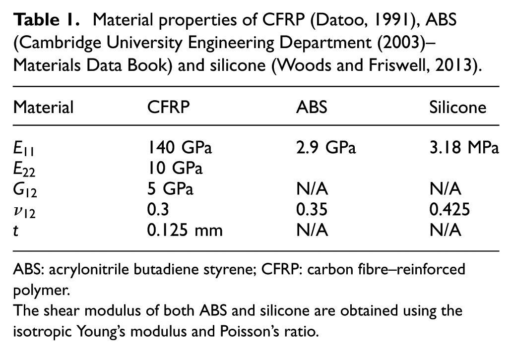
ABS: acrylonitrile butadiene styrene; CFRP: carbon fibre–reinforced polymer.
The shear modulus of both ABS and silicone are obtained using the isotropic Young’s modulus and Poisson’s ratio.
Analytical model
The following section introduces the fundamentals of plate theory that are used to model the behaviour of the FishBAC, as well as the specific procedure that is followed to obtain the displacement fields, including an introduction to the Rayleigh–Ritz method for structural analysis (Whitney, 1987). Furthermore, this section introduces the assumed shape functions and the global boundary conditions that are implemented in the analytical formulation.
Rayleigh–Ritz method
The Rayleigh–Ritz method is a variational method that can be used to approximate solutions to partial differential equations based on energy formulations. Its foundation lies in the principle of conservation of total energy in a closed system. From a mechanics point of view, this implies that the sum of the strain energy of the body and the kinetic and potential energies due to external loads is a stationary value (Ilanko et al., 2015; Whitney, 1987). This approach assumes that no frictional losses exist, which is a reasonable simplifying assumption for many types of structures.
For an initially flat plate, these energy formulations can be written in terms of a total energy expression that is a function of the plate displacement’s

where
Since the scope of this work is to analyse the static displacement of composite FishBAC structures, kinetic energy is neglected for the time being, although it can still be added in later if dynamics are of interest.
Energy definitions
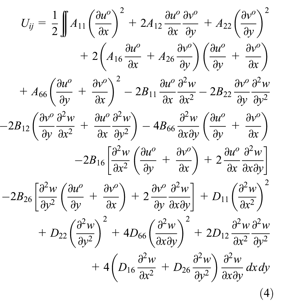
For an elastic body, the total strain energy is defined as the integral of the sum of the products of stresses and strains across the volume of the body as seen in equation (2)
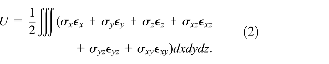
As mentioned earlier, the presented analytical model is based on Kirchhoff–Love plate theory. Therefore, through-thickness and transverse shear strains are neglected (i.e.
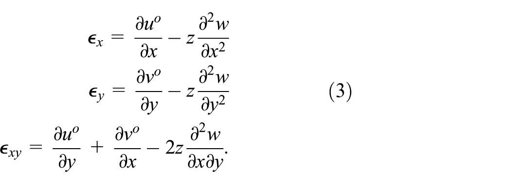
This assumption leads to a mathematical expression in terms of the plate’s displacements and its derivatives and the stiffness terms, which in this case are expressed in terms of the ABD matrix, when CLT is implemented (equation (4)). The ABD matrix describes the stiffness of the composite laminate; it combines both material and geometric stiffness in a single expression (Hyer, 2014).
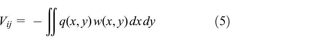
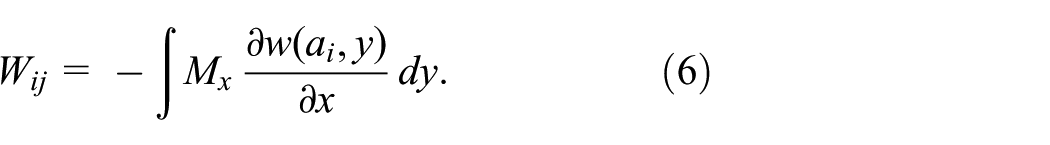
Furthermore, the net aerodynamic pressure distribution acting on the FishBAC (which is found separately using an aerodynamic solver, for example, panel methods or computational fluid dynamics (CFD)) can be treated as a transverse pressure distribution, on the plate, with both variations in x and y. The potential energy due to transverse pressure loading (i.e. force per unit area) is defined as the integral of the pressure times the transverse displacement across the surface area (equation (5), Whitney, 1987). The potential energy due to the actuation moments at the trailing edge depends on the first derivative of the transverse displacement along the bending direction and the applied moment intensity Mx (equation (6), Mansfield, 1989). These three expressions can be found as follows:
Displacement fields and shape functions
The energy definitions presented in the previous subsection are all in terms of the plate’s displacement and its derivatives, the material and geometric stiffness represented by the ABD matrix terms (equation (4)) and external loads (equations (5) and (6)). In this case, both material properties and external loads are known and treated as inputs, while the displacements are unknown and, therefore, their shapes need to be determined. Within the context of Rayleigh–Ritz method, all three displacements (i.e. uo, vo and w) are normally defined in the form of three sets of double summations of terms in the x- and y-direction that satisfy compatibility conditions (equation (7))
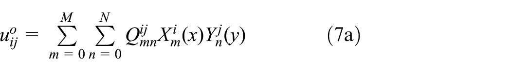
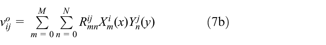
where
Previous studies have considered several types of shape function. A common approach in plate mechanics for solving the plate’s differential equation is to assume that the displacement occurs in a periodic form, which makes the use of cosine and sine Fourier series expansions convenient as it allows for closed-form solutions to the differential equation. Several examples of using periodic functions are presented in Green (1944), Fo-Van (1980), Bhaskar and Kaushik (2004) and Khalili et al. (2005), among others.
Another alternative to periodic functions is using orthogonal polynomials. They present better convergence rates when deflections do not occur in a periodic way as they can capture localised features using less expansion terms. In the context of plate mechanics, successful examples of implementing generic orthogonal polynomials are presented by Bhat (1986) and Rango et al. (2013) performed static analysis of fibre-reinforced composite plates using orthogonal polynomials.
Furthermore, a specific set of polynomials, known as the ‘Jacobi family’, are commonly used in structural mechanics. This ‘family’ includes the Gegenbauer polynomials, which is a special case of the Jacobi polynomials and the Chebyshev and Legendre polynomials, which themselves are a special case of the Gegenbauer set (Abramowitz and Segun, 1968; Boyd and Petschek, 2014).
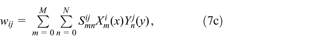
From the structural mechanics point of view, Legendre polynomials have been successfully implemented in several cases, for example, in predicting buckling of highly anisotropic plates (Wu et al., 2012) and discontinuous panels with variable stiffness (Coburn et al., 2014), analysing displacements of variable stiffness beams and plates under transverse pressure loading (O’Donnell and Weaver, 2017) and also in capturing step changes in thickness (Vescovini and Bisagni, 2012). However, their integrals have an exact value of zero when integrated across their normalised domain. This would imply that there is zero net work when an uniform transverse pressure distribution and external moments are applied (equations (5) and (6)). On the other hand, Chebyshev polynomials do not present this property. Therefore, the shape functions that are implemented in this analytical model are Chebyshev polynomials of the first kind, defined as (equation (8))
where n corresponds to the polynomial order.
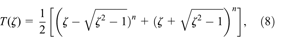
One important aspect to consider during the analysis is that since Chebyshev polynomials are normalised and defined from
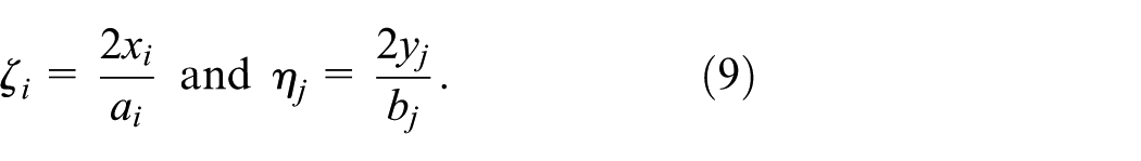
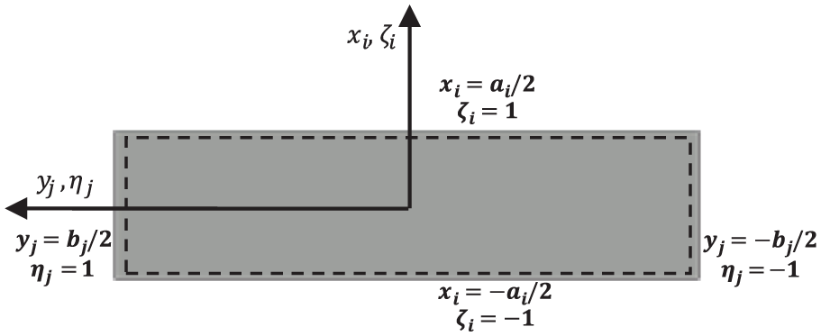
Coordinate transformation, from physical
Global boundary conditions
The FishBAC morphing trailing edge section is modelled as a cantilever plate (Figure 7) clamped to the rigid forward section of the wing. This constraint implies that the root of the FishBAC’s plate must present zero displacement and rotation. Since the Chebyshev polynomials do not naturally meet this condition, the expansion in the chordwise polynomial functions must be modified to enforce the clamped boundary at the first row of plate partitions at the root. Jaunky et al. (1995) introduced the concept of using a circulation function to enforce boundary conditions at any location

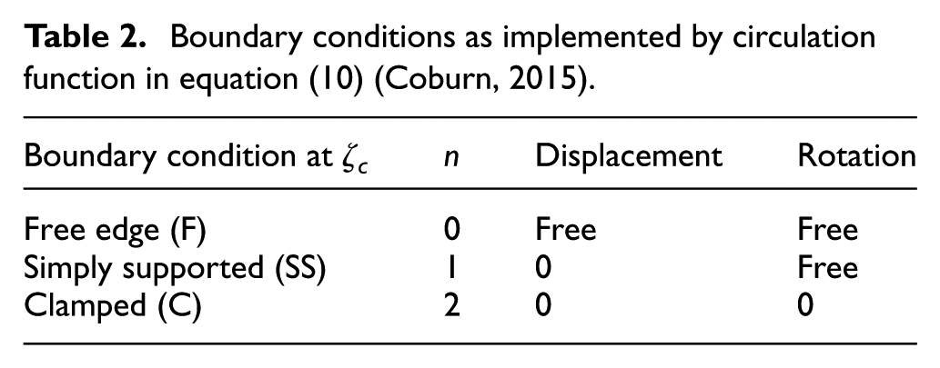
where the value of n is set depending on the nature of the boundary condition of the
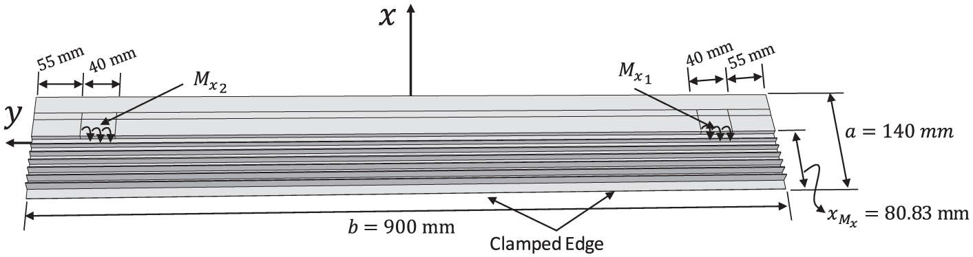
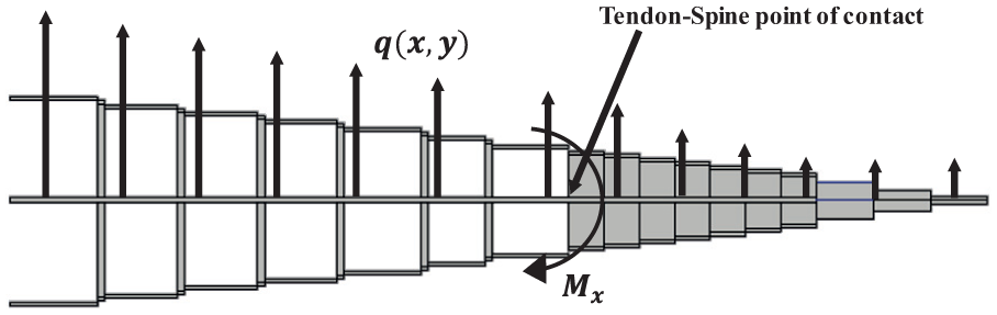
Global coordinate frame of the FishBAC, including global dimensions and locations at where actuation moments are applied. Note that the location where the actuation moments correspond to the tendon-spine points of contact (tendons not shown).
Boundary conditions as implemented by circulation function in equation (10) (Coburn, 2015).
Stiffness discontinuities and local boundary conditions
The stiffness of the FishBAC is inherently discontinuous due to the presence of the stringers, which implies that the energy balance presented in equation (1) has to be calculated in each section of uniform stiffness as the ABD matrix terms in equation (4) vary significantly between regions with and without stringers. Note that since independent shape functions are used for each individual section (equation (7)), a coordinate transformation from the physical to the normalised frame has to be performed in each partition, individually. Hence, a local coordinate system is defined at the centre of each element and then individually mapped to local
In structures with stiffness discontinuities, shear force and bending moments at each ‘joint’ must be continuous when approached from either side of the boundary. However, due to the ‘step’ change in both geometric and material stiffness, curvatures are not continuous. These types of structures are known as ‘C1-continuous’, where displacement and rotations at local boundaries must be continuous, but higher order derivatives do not. Since Chebyshev polynomials do not inherently meet this type of structural continuity at local boundaries, these have to be enforced by other means (Coburn, 2015).
There are two common approaches for ensuring displacement and rotation continuities: Lagrange multiplier method or Courant’s penalty method (Ilanko et al., 2015). The former one consists of deriving a set of constraint equations that are scaled by unknown coefficients, called Lagrange multiplier, that represent the exact value that the constraints need to be weighted by to enforce continuity. The latter approach consists of using a penalty energy term, analogous to joining each section with a torsional/displacement springs and accounting for the spring energy that is needed to enforce displacement and rotation compatibility (i.e. continuous displacements and rotations). Due to the number of equations and separate Lagrange multipliers that would be needed, the Courant’s penalty method in form of spring penalty energies is is selected in this opportunity. It is worth noting that while these are not the only methods to enforce the ‘C1-continuity’ (e.g. each individual polynomial set could be modified so they naturally meet this condition), these two approaches are by far the most common in the literature as modifying each polynomial set would be difficult to setup and computationally expensive.
Courant’s penalty method
As mentioned in the previous subsection, each one of the plates sections is assumed to be joined with an artificial penalty spring with a stiffness equal to
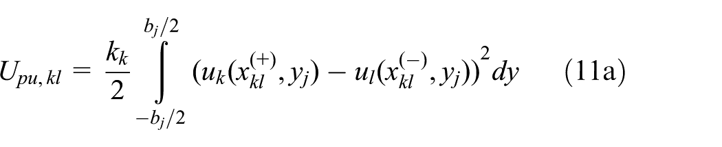
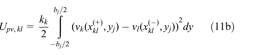
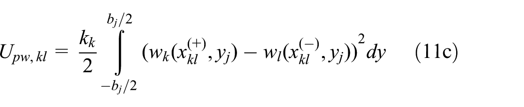
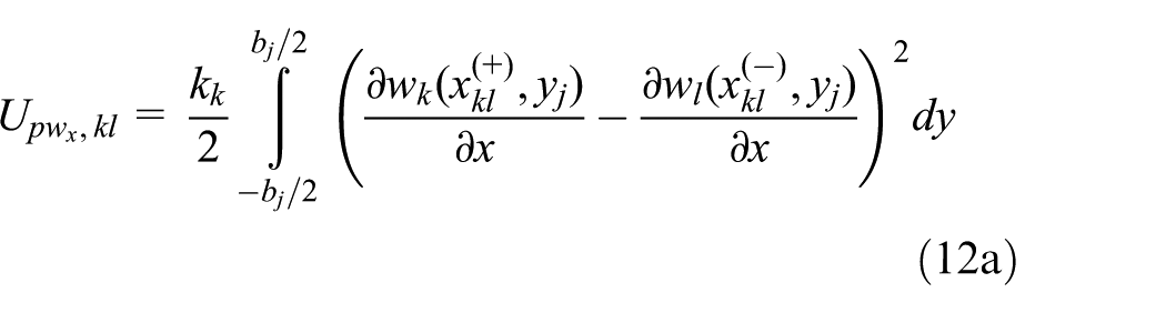

where
As mentioned earlier, the values of

Previous studies have selected the stiffness of penalty springs based on convergence studies of their models. Coburn (2015) performed a convergence study based on percentage difference with respect to FEM and estimated that the model was accurate for a penalty stiffness between
Convergence studies for selecting the magnitude of both chordwise and spanwise penalty springs were performed using the FishBAC’s geometry. These studies showed that for four different spine composite ply stacking sequences, a value of
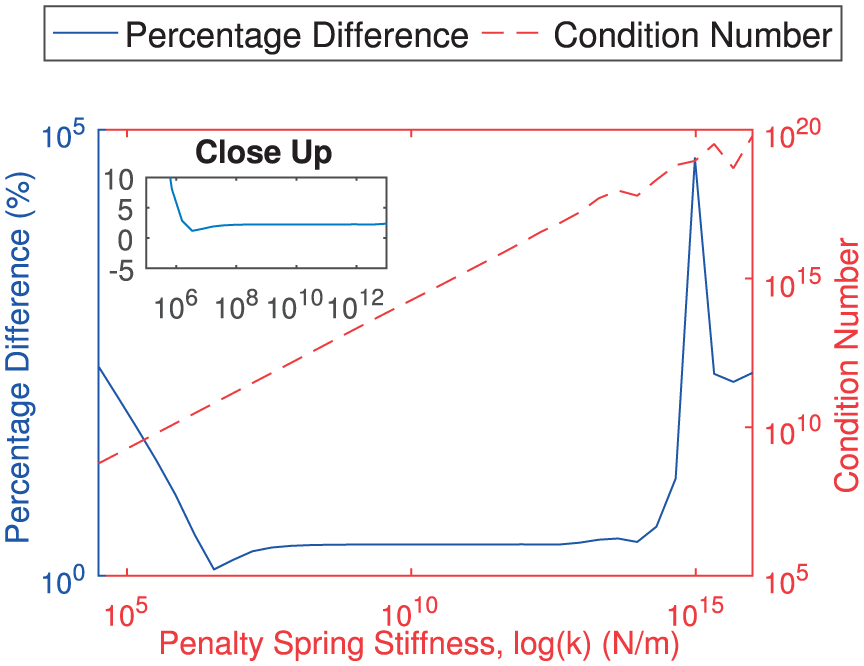
Convergence study for selecting the magnitude of the penalty springs for Chebyshev terms of
Furthermore, in order to mitigate numerical errors due to high condition number, the coefficient matrix is normalised by dividing each individual row KT by its root mean square (RMS), as defined in equation (14) (Groh, 2015). In this particular application, this normalisation reduces the condition number of the coefficient matrix by at least four orders of magnitude
Principle of minimum potential energy
As previously stated, the Rayleigh–Ritz method is based on the assumption of conservation of total energy in a closed system. This approach implies that the sum of energies defined in equation (1) has a stationary value. Therefore, differentiating the total energy formulation with respect to any of the unknown constant shape function amplitudes,
Model implementation
The structural model described in the previous sections was implemented using MATLAB® R2016a, on an Intel® Core™ i7-4790 3.60 GHz CPU processor, using a 64-bit OS with 16 GB of physical memory. The geometric dimensions of the model were selected based on a 600 × 900 mm NACA 2510 wing tunnel model that was used for previous experiments. Out of those 600 mm of chord length, the last 140 mm corresponds to the FishBAC, which implies that the morphing device starts at 76.6% of chord length. In other words, the first 460 mm of chord length from the leading edge corresponds to the rigid section of the wing, which is not being modelled in this work.
The derivatives of the shape functions are computed analytically, while the integrals in equations (4) and (5) are computed using ‘integral2’ a two-dimensional adaptive quadrature MATLAB built-in function. Furthermore, the integrals at the partition boundaries are needed for calculating the work due to actuation moments (equation (6)) and penalty energy terms (equations (11) and (12)). However, the analytical derivative of the Chebyshev polynomial recurrence formula (equation (8)) cannot be directly integrated at these locations as it is indeterminate due to a zero denominator. This limitation is solved by calculating the limit of the Chebyshev polynomial as its two boundaries are approached (i.e. at
It is important to mention that all the integrals were performed in the non-dimensional reference frame, defined from
Furthermore, the FishBAC was divided into a total of 115 partitions: 23 in the chordwise direction and 5 in the spanwise direction. This many chordwise partitions allows all stiffness discontinuities due to stringers to be captured and also to ‘discretise’ the solid trailing edge thick section to avoid steep changes in thickness. In terms of physical dimensions, the spine has a uniform stiffness of 0.75 mm, while each stringer height varies in accordance with the aerofoil thickness distribution, having values that range from 14 to 7 mm. Finally, a uniform skin thickness of 0.5 mm maintains the NACA 2510 aerofoil section. It is important to mention that even though this structural model was developed around the FishBAC concept, it can be easily adapted to model any plate-based structure, regardless of its level of discontinuity, stiffness properties, boundary conditions or dimensions.
Finally, the authors consider that a targeted accuracy between 5% and 10% is acceptable for initial design and elastic tailoring. However, the authors are also aware that this target may need to change depending on the sensitivity of the aerodynamics to structural deflections. Future wind tunnel tests and fluid–structure interaction models will give a better insight of the accuracy needed for modelling this morphing device.
A top view diagram of the partitions, with their respective dimensions, can be found in Figure 9. It is important to mention that the number of partitions and dimensions, stringer spacing and so on can be easily modified by manually changing the input parameters of the MATLAB script file. Also, since the integrals are not computed for each partition individually, increasing the number of partitions does not have a significant impact on the computational cost of the simulation.
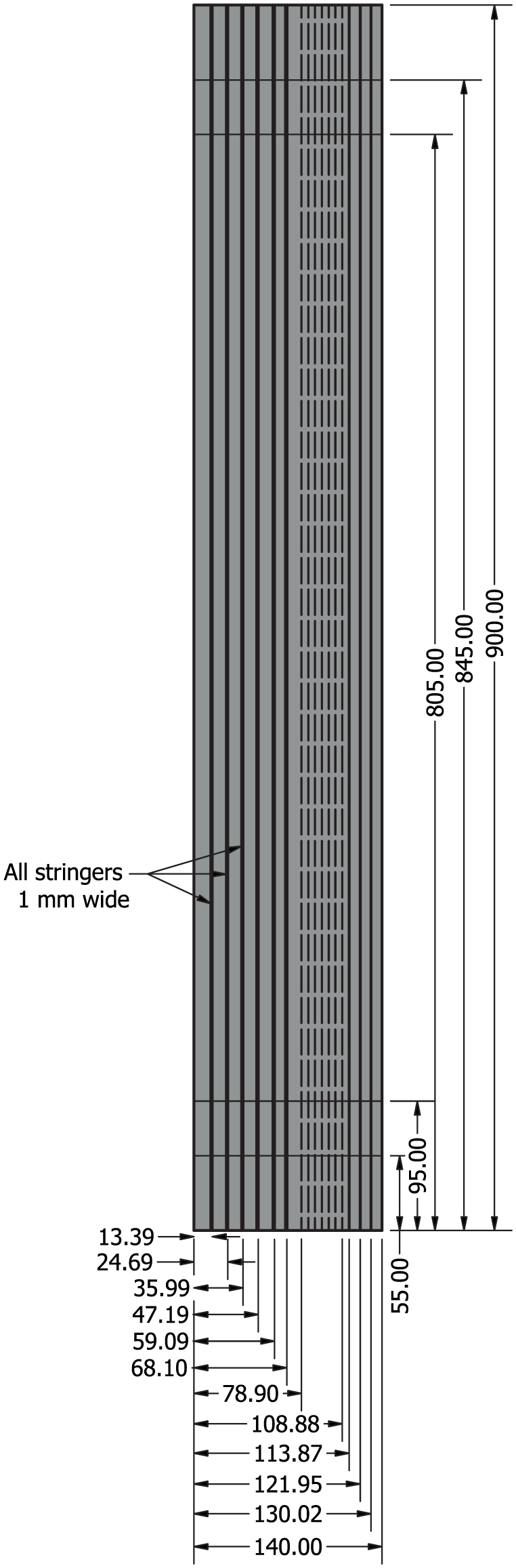
Top view of the analytical model geometry (with local dimensions). A total of 23 chordwise and 5 spanwise partitions, respectively, are used to model the complex geometry of the FishBAC. All dimensions are in millimetre.
Validation: finite element model
A FEM model of the FishBAC was developed, using ABAQUS/CAE® version 6.14-1, to validate the analytical model. As this FEM model is based on the true FishBAC geometry, comparing the analytical model to it will simultaneously test both the simplified geometry (Figure 5) and mathematical assumptions that are implemented in this analytical model. The FEM model consists of a combination of shell, continuum shell and solid elements that are joined together as a single part. The composite plate, stringers and the skin of the compliant section are modelled using four-node shell (S4R) elements. Furthermore, the spine’s material is defined as a composite laminate (i.e. shell elements with material defined on a ply-by-ply basis), while both the skin and the stringers are modelled as isotropic (Table 1).
The ‘thick’ section of the trailing edge is modelled using a combination of solid 8-node (C3D8R) elements, for the isotropic parts, and continuum shell (SC8R) elements, for the laminated composite parts (Figure 10). This is due to the fact that this region contains a section of the composite spine that is located in between solid isotropic material. A geometrically non-linear analysis was performed for several different spine stacking sequences under a range of uniform pressure distributions, ranging from 20 to 500 Pa. The nodal displacements along the free edges were tracked and extracted to allow for comparison to the analytical model. A fully clamped boundary condition was applied to the root of the FishBAC. Furthermore, the FishBAC’s skin is pre-stretched by 10% to minimise out-of-plane deflections under aerodynamic loading and to avoid buckling in compression. In order to simulate this, the skin is prestressed in the FEM model by applying a prescribed uniform, in-plane predefined stress field equal to the Young’s modulus of the skin times 10% strain in the chordwise direction. Spanwise stress/strain due to Poisson’s ratio effect is not considered, as during the manufacture of actual FishBAC skins, the skin is free to contract in the spanwise direction before it is bonded to the structure. A convergence study was performed to set the element size used for comparison by varying the global element size of the mesh and calculating the percentage difference for each increment. In this study, convergence is achieved when the average percentage difference in tip displacements vary less than 0.5% for two consecutive increments in mesh density.
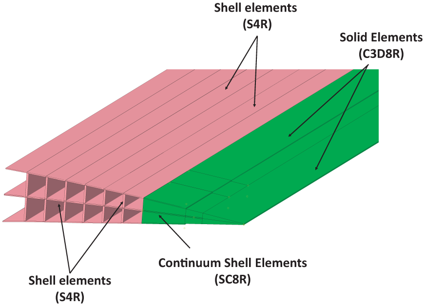
Schematic of the type of elements that are used to model the behaviour of the FishBAC’s static displacement. Solid and continuum shell elements are displayed in ‘green’ colour, while shell elements are displayed in ‘pink’ colour.
Loading condition
One of the assumptions in the structural analysis of the FishBAC is that the aerodynamic pressure distributions on the upper and lower skins are translated directly to the spine. This equivalent pressure is found by subtracting the top surface pressure distribution from the bottom one (equation (16)). This approach has one disadvantage: it does not allow the out-of-plane deformation of the skin, under aerodynamic loads, to be modelled. However, for the level of fidelity and purpose of this tool (robust and efficient fluid–structure interaction for design and optimisation), these skin deformations would not be captured with the aerodynamic tools that will be used. A full CFD analysis is needed to estimate the skin deformation between stringers, which would add significant computational expense. A potential alternative is to separately model the skin deflections using CFD and superimpose the results with the current structural model. Finally, as previously mentioned, pre-tensioning the skin mitigates the effects of skin deformation on the aerodynamic loads, as it increases its stiffness, reduces out-of-plane skin deflections and prevents buckling when in compression
Furthermore, the actuating loads are applied as point moments at the location where the tendons meet with the spine. Figure 11 displays the type of loading applied in both analytical and FEM models, while Figure 7 shows the locations where the external actuation moments are applied, including their moment arms with respect to the clamped edge. For the purpose of this initial investigation,
The magnitude of the transverse pressure loadings was selected based on preliminary FEM simulations, targeting similar maximum deflections of 4–5 mm for all four spine material configurations, allowing for direct error comparison between all four cases. Note that the highest pressure value applied to each case is similar or higher to the values that the composite wind tunnel model of similar dimensions would experience at Mach 0.15

Results and discussion
The analytical model presented in this article is compared against a non-linear finite element analysis of the FishBAC under uniform pressure distribution and actuating moments. In addition to the resulting displacement fields, a convergence study in terms of Chebyshev polynomial terms is presented. In these sets of results, two types of errors are reported: the maximum absolute value percentage difference and the RMS percentage difference between analytical and FEM results.
Polynomial term convergence
A convergence study of Chebyshev polynomial terms against the converged FEM results is presented for four different spine material configurations: isotropic ABS,
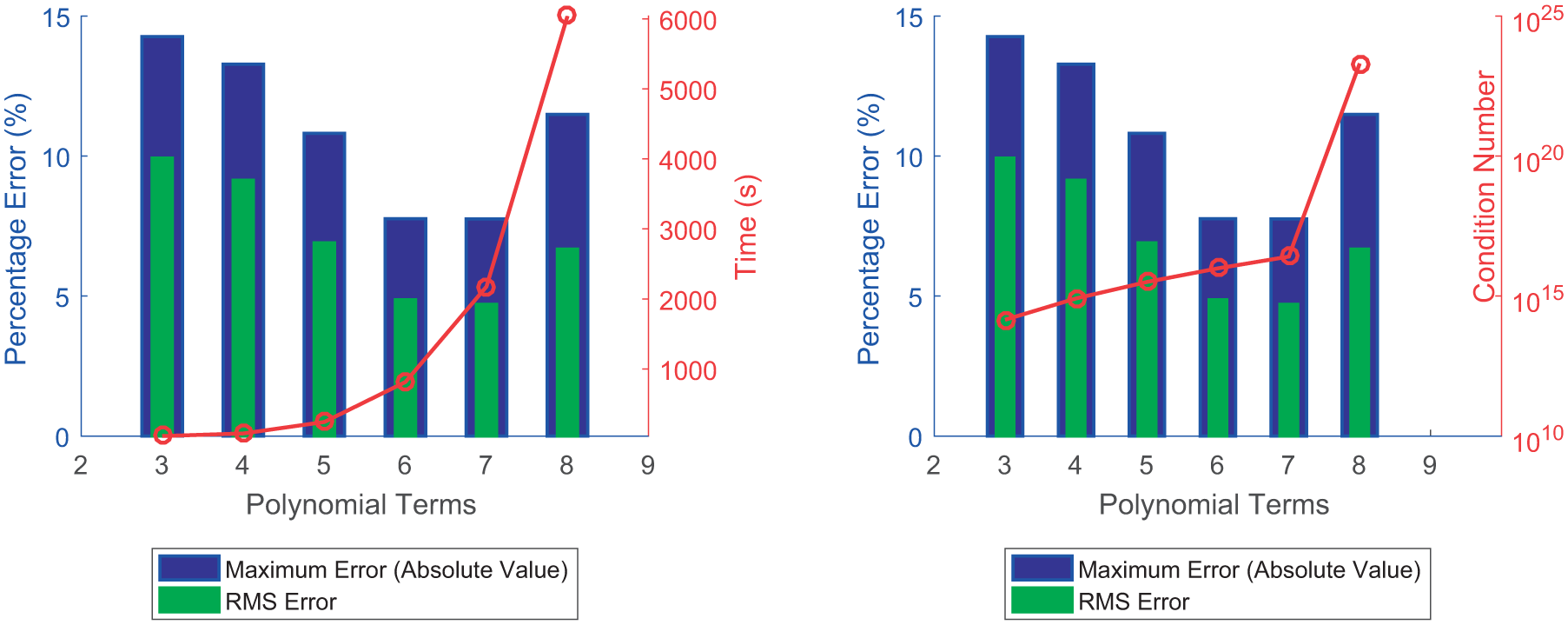
Convergence study: comparison between analytical and geometrically non-linear FEM results for a spine’s stacking sequence of [45/45/45] S .
Comparison of analytical and geometrically non-linear FEM results in function of Chebyshev polynomials terms (polynomial order).
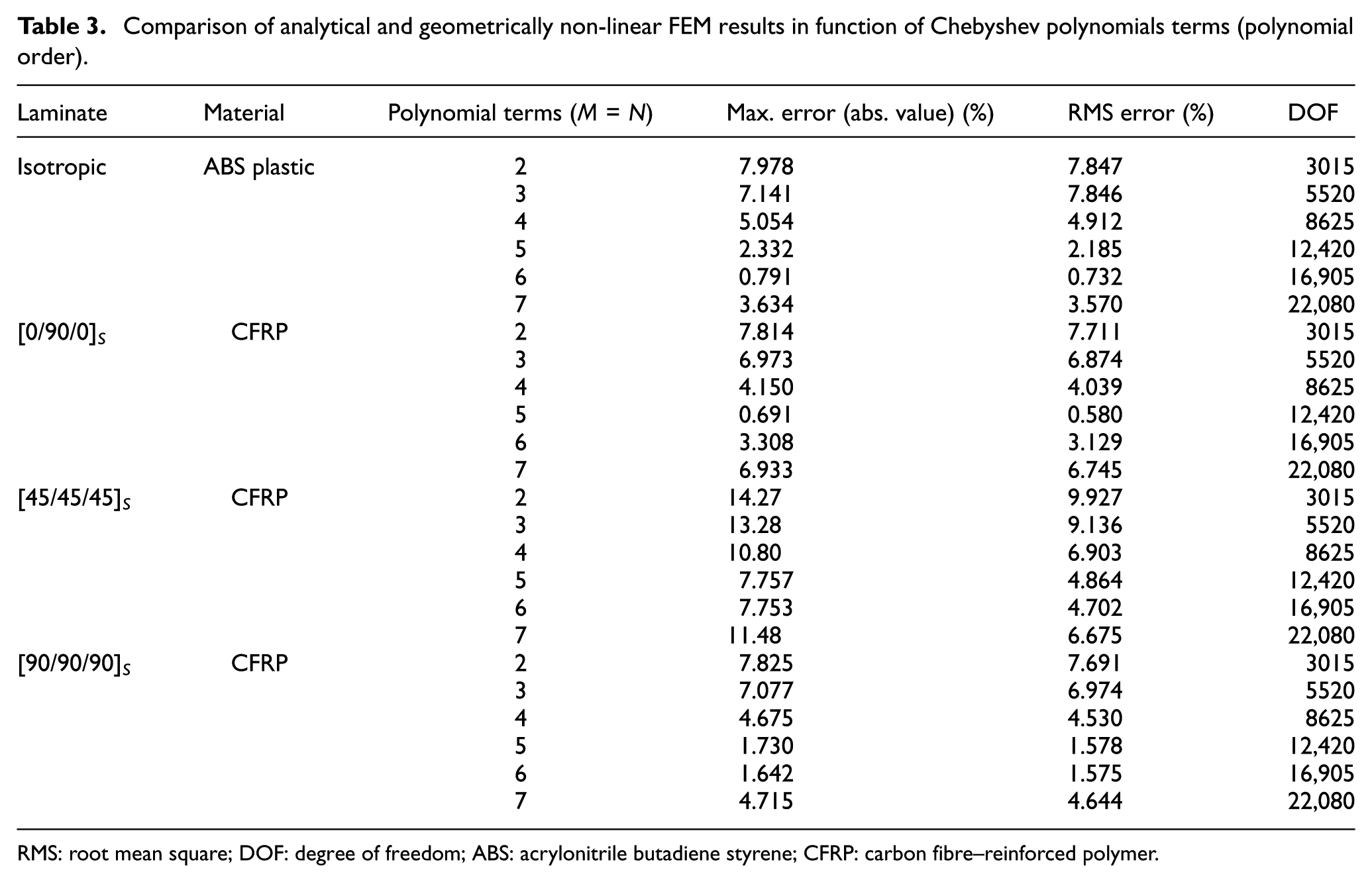
RMS: root mean square; DOF: degree of freedom; ABS: acrylonitrile butadiene styrene; CFRP: carbon fibre–reinforced polymer.
Results show that for all four spine configurations, a RMS error of less than 4.9% can be achieved when five Chebyshev polynomial terms in both chordwise and spanwise direction (i.e. M = N = 5) are used. In general, it is observed that adding a sixth term has a positive effect in further reducing the RMS percentage error, at the expense of doubling the computation time. On the other hand, there is a significant increase in error when adding a seventh polynomial term. This also corresponds to an increase in condition number of about seven orders of magnitude in all four cases, as observed in Figure 12. It can be concluded that the proposed analytical model has a limit of six Chebyshev polynomial terms, as further increasing the number of polynomial terms yields severe ill-conditioning. Finally, it can be observed that results within ≈7% RMS error can be obtained when four polynomial terms are used, which represents an attractive case for future optimisation studies as this case represents a 66% reduction in computational time than when five terms are used. It is also attractive in terms of computational effort with respect to the FEM, as it requires less than 8% of the total number of DOFs as the converged FEM. As a commercial software package, ABAQUS/CAE (FEM) benefits from a highly optimised solution process for its equations of motion, but further optimisation of the solution methods for the process shown here is likely to yield significant improvements in solution time. This approach is in addition to the benefits of simple, parameter-driven geometry/material definition (ideal for optimisation and aeroelasticity) provided by the proposed method.
Regarding the type of error, it is observed that the RMS and the maximum absolute value percentage error are very similar in the isotropic,
Finally, the difference in percentage error (Table 3) among the four material configuration is primarily due to the degree of material anisotropy and the presence of transverse shear in the
Uniform pressure loading
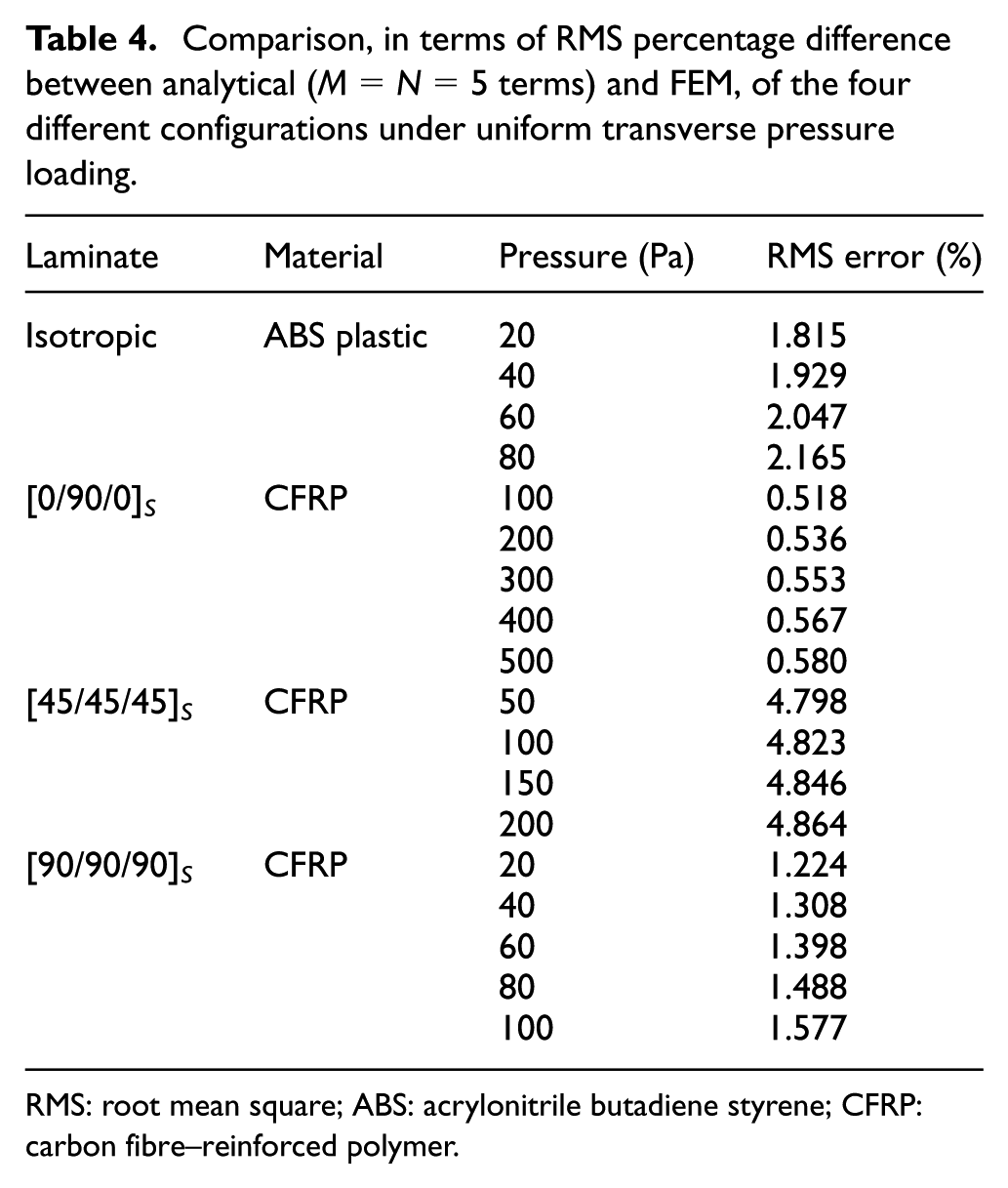
Uniform transverse pressure was applied to the same four laminates presented in the previous subsection. The RMS percentage difference along the spanwise
Table 4 shows that the RMS error remains stable as the load increases. Furthermore, it can be observed that the most anisotropic layup (i.e.
Comparison, in terms of RMS percentage difference between analytical (
RMS: root mean square; ABS: acrylonitrile butadiene styrene; CFRP: carbon fibre–reinforced polymer.
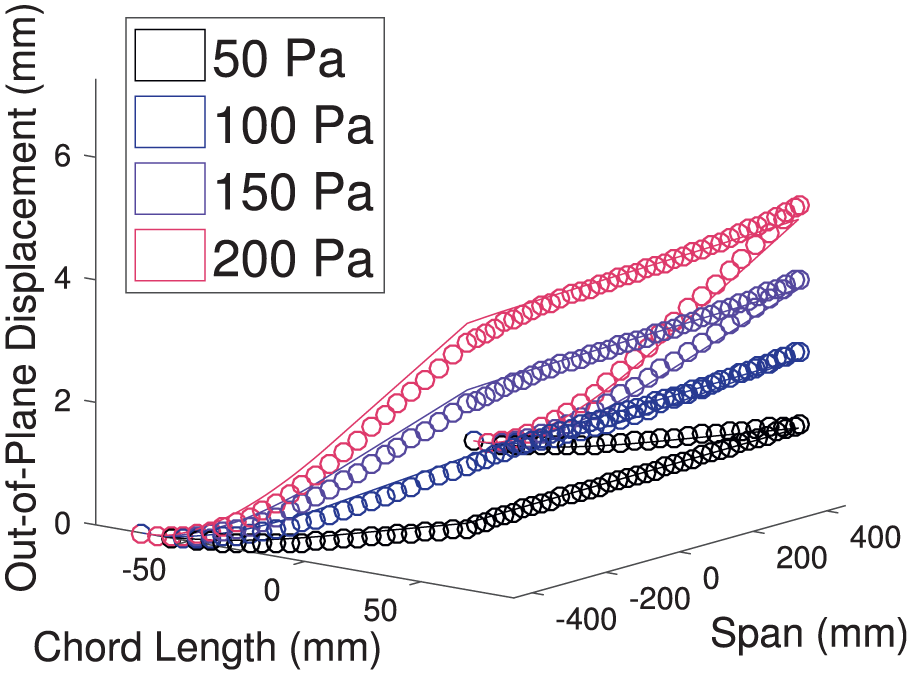
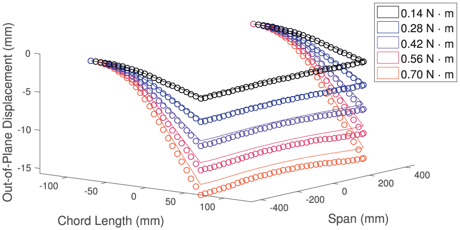
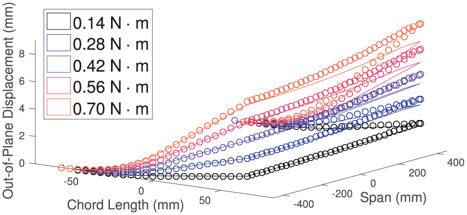
Comparison between analytical (solid) and FEM (
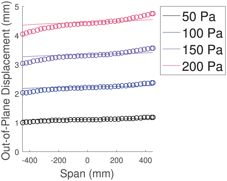
Analytical (solid) versus FEM (
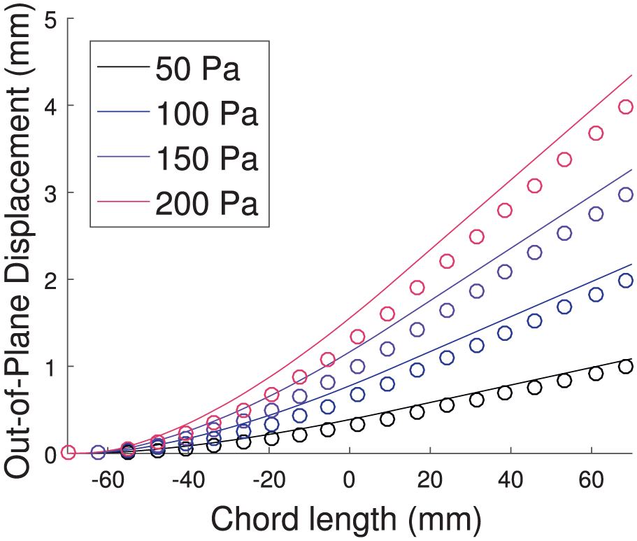
Analytical (solid) versus FEM (
Even though localised discrepancies can be observed along the spanwise edge, the global deformation of the FishBAC is properly captured (Figure 13). As mentioned earlier, properly capturing the global deformation is a priority for this application, as this would drive any change in aerodynamic loads.
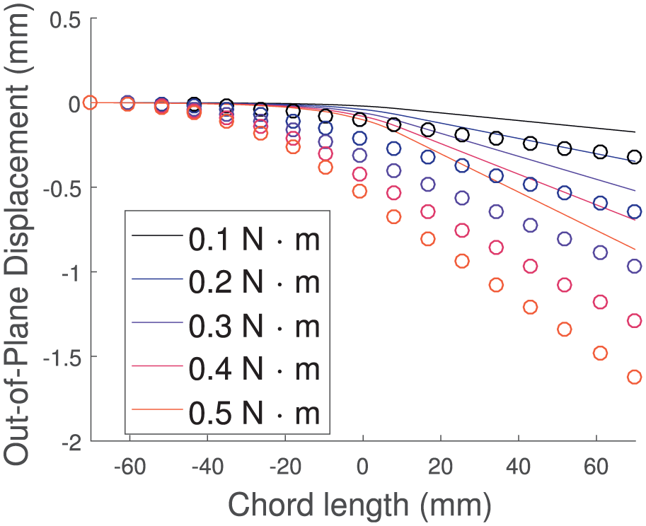
On the other hand, the
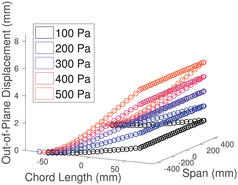
Comparison between analytical (solid) and FEM (∘) displacement field, for a
Analytical (solid) versus FEM (∘) displacement along the spanwise edge
Analytical (solid) versus FEM (∘) displacement along the chordwise edge
Actuation moments
A comparison of analytical versus FEM displacements, under input moments, was performed for the two most compliant laminates in the chordwise direction (i.e. isotropic and
Comparison, in terms of RMS percentage difference, between analytical (
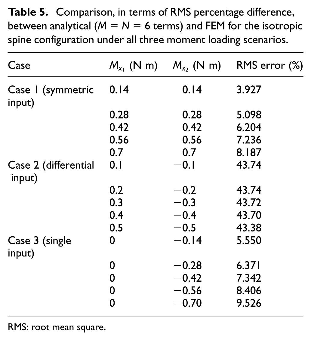
RMS: root mean square.
Comparison in terms of RMS percentage difference between analytical (
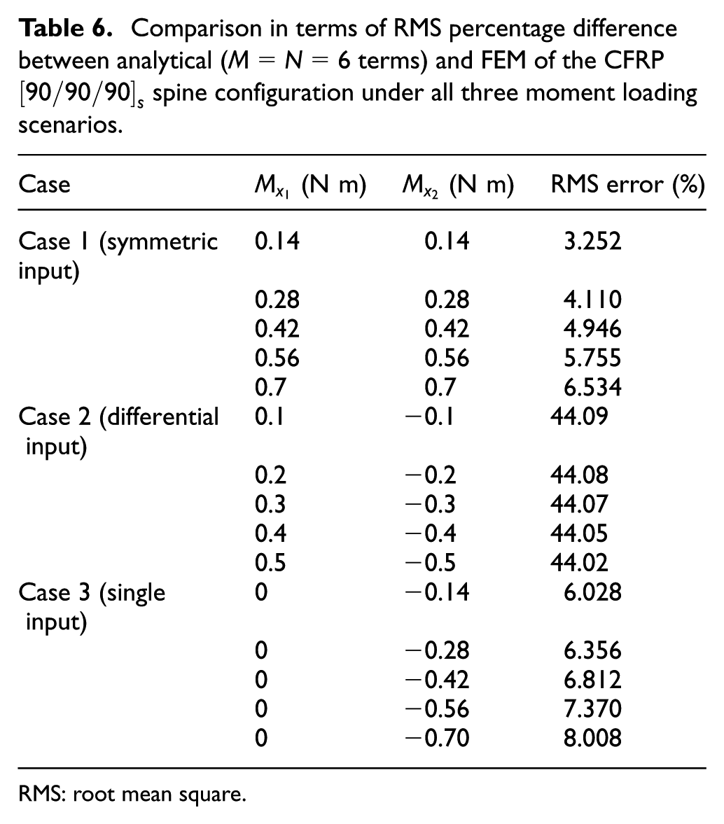
RMS: root mean square.
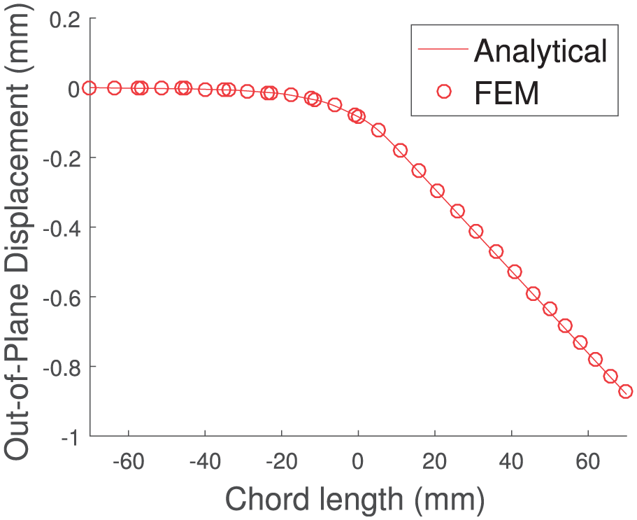
When comparing displacement fields, it is observed that Case 1 and Case 3 show similar behaviours to FEM, in terms of chordwise and spanwise edge displacement and slopes, with an overall RMS error of less than 8.6%. Figure 19 shows the displacement field of the
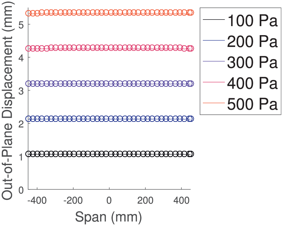
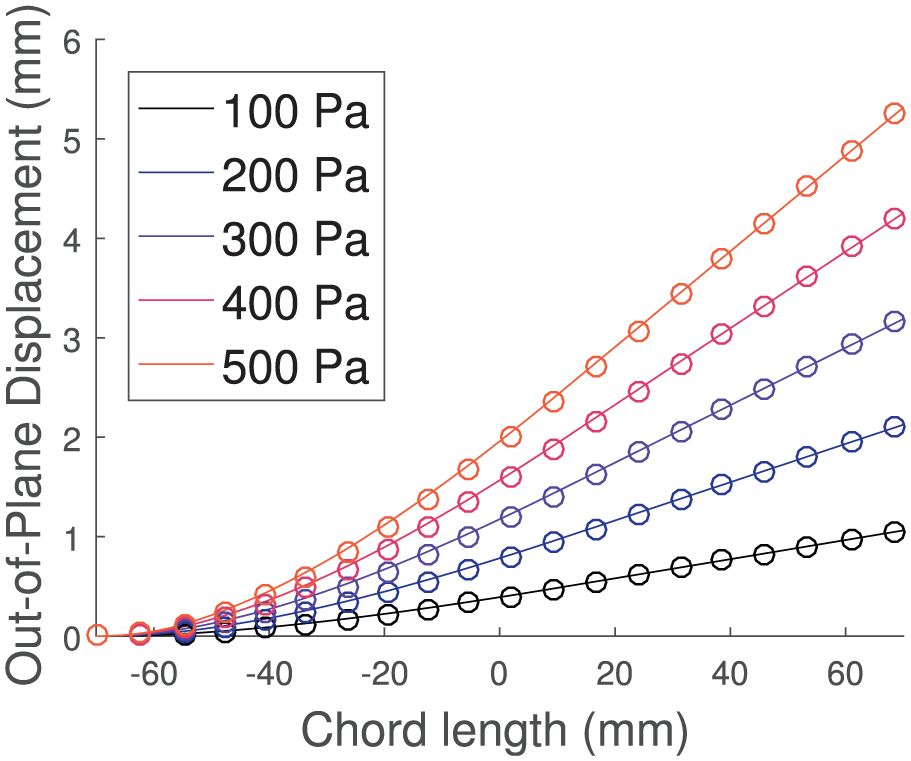
Analytical (solid) versus FEM (∘) for a [90/90/90] S spine’s laminate under uniform positive actuation inputs.
Analytical (solid) versus FEM (∘) for a [90/90/90]
S
spine’s laminate under a single negative
On the other hand, Case 2 (i.e. differential moment inputs) shows significant discrepancies in terms of RMS error along the spanwise free edge and the deformed shape. Tables 5 and 6 show RMS errors as high as 44%, for the isotropic and
Analytical (solid) versus FEM (∘) deflection along chordwise edge y =–b/2, for a [90/90/90] S spine’s laminate, under differential moment inputs.
Unlike the other load cases that have been analysed, the differential moment input case does present transverse shear as these moment inputs generate a net torque along the spine’s x-axis. As a consequence, shear flow is induced, resulting in transverse shear stresses and strains (i.e.
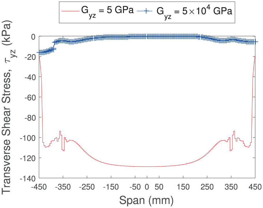
Transverse shear stress
Analytical (solid) versus FEM (o) displacement along chordwise edge
Computational comparison: model size and convergence study
A final comparison, in terms of DOFs between analytical and FEM model, is presented in this section (Table 7). The FEM’s DOFs correspond to a converged mesh and include all boundary conditions and constraints applied during the analysis. It is observed that among all cases, the analytical model reduces the DOF that need to be solved by at least 84%, compared to a FEM converged mesh. Note that for the
Analytical versus FEM degrees of freedom.
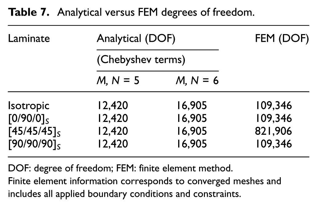
DOF: degree of freedom; FEM: finite element method.
Finite element information corresponds to converged meshes and includes all applied boundary conditions and constraints.
A reduction in DOFs is not only a measure of the efficiency of the analytical model, as it can obtain converged solutions (except when transverse shear due to differential moment inputs exist) with a smaller linear system, but also significantly decreases the amount of RAM memory required to obtain static deformations.
Conclusion
An efficient and mesh-independent two-dimensional analytical model for predicting the static behaviour of the FishBAC trailing edge device has been developed. The model is capable of analysing fully anisotropic FishBAC geometry and material configurations and predicting the in-plane and out-of-plane displacement fields under external two-dimensional transverse pressure loading and applied actuation moments. It achieves the static modelling by condensing all of the geometric and material features of the FishBAC into a single system of linear equations, obtained using Rayleigh–Ritz method.
Its novelty lies in capturing the complex structure of the FishBAC by discretizing its geometry into a series of individual plates, each one with an equivalent stiffness at the mid-plane, that are joined together using a series of artificial penalty springs. Furthermore, it allows for rapid modification of the structural and material parameters of the FishBAC (e.g. spine stacking sequence, dimensions, stringer spacing), and due to its mesh-independent and analytical nature, it can compute converged displacement fields by solving a fixed number of linear equations that only vary with the polynomial order of the assumed shape functions.
Results show that under uniform pressure loading, the analytical model converges in five Chebyshev polynomial terms, with a percentage error under 4.8% with respect to FEM, using 84% less DOFs. Furthermore, errors in predicting large deflections due to actuation loads range from 3% to 8%, except when a differential moment input is applied. This load case results in a net torque on the FishBAC’s spine, causing transverse shear deformations along the y–z plane. Significant discrepancies exist in this specific load case, and they are due to Kirchhoff–Love plate theory’s inability to capture any through-thickness strains.
Although the analytical model has been developed around the FishBAC morphing trailing edge concept, this approach can be used to model any plate structure, regardless of its level of discontinuity or material properties. Furthermore, this model opens the design space for future design iterations of the FishBAC, not only allowing for the use of composite laminates, but also of core materials (e.g. sandwich configuration). Also, since it is built around Rayleigh–Ritz method, dynamic analysis can be introduced by accounting for kinetic energy, which will be required in the near future to model deflections under unsteady aerodynamic load cases. Also, Rayleigh–Ritz Method can be used to perform both static and dynamic aeroelastic studies.
In summary, the analytical model represents a powerful, robust and fast tool for future design and optimisation of the FishBAC as the structural and material parameters can be easily modified. Future work will address the limitations to accurately predict deflections when transverse shear exist; methods, such as FSDT, will be considered. Finally, this model will act as the foundation of a fluid–structure interaction model that will be able to couple deflections with aerodynamic loads.
Footnotes
Acknowledgements
The first author would like to thank Dr Matt O’Donnell for his support on the numerical implementation of Rayleigh–Ritz method in MATLAB and Mr Sergio Minera for his assistance on transformations between coordinate systems. The authors would also like to thank the reviewers for their constructive suggestions to improve the quality of this article.
Declaration of conflicting interests
The author(s) declared no potential conflicts of interest with respect to the research, authorship and/or publication of this article.
Funding
The author(s) disclosed receipt of the following financial support for the research, authorship, and/or publication of this article: This work was supported by the Engineering and Physical Sciences Research Council through the EPSRC Centre for Doctoral Training in Advanced Composites for Innovation and Science (grant number EP/L016028/1). The second author would like to acknowledge the Royal Society for the Royal Society Wolfson Merit award and also the Science Foundation Ireland for the award of a Research Professor grant. The third author would like to acknowledge the Royal Academy of Engineering for the Research Professorship award.
Data Access Statement
All underlying data are provided in full within this paper.