
Abstract
This article attempts to test the environmental Kuznets curve (EKC) for export diversification and river water pollution (proxied by biochemical oxygen demand) for India during the period from 1986 to 2019. Over the past decade, India’s merchandise exports have been dominated by pollution-intensive industries such as mineral fuels, pharmaceuticals, nuclear reactors, organic chemicals and electrical machinery, iron and steel, and textiles. Additionally, India’s export mix is weakly diversified or a small number of commodities form the merchandise export basket. River water pollution is one of the gravest ecological threats in this country. Although a host of reasons define this ecological devastation, this study attempts to investigate if the weakly diversified, pollution-intensive export basket has any link with biochemical oxygen demand.
Dickey–Fuller (ADF) and Philip–Perron (PP) tests are employed to determine the stationary properties of the variables and the autoregressive distributed lag (ARDL) cointegration test, as well as the bounds test to check the short- and long-run cointegration.
Findings suggest that (a) export diversification is strongly cointegrated with biochemical oxygen demand both in the short and in the long run, and (b) the conventional inverted U-shaped EKC was not validated. Furthermore, a weakly diversified export basket increases water pollution.
Suggested policy initiatives to combat industrial water pollution include the introduction of economic instruments. The water pollution abatement experience of industrial clusters suggests that radical institutional and governance reforms are paramount for successful policy reforms. Finally, there is a need to reduce the export commodity basket concentration not just to insulate the economy against global dynamics but also for achieving the goal of sustainable development.
Introduction
Developing countries face a difficult trade-off in the choice between rapid economic growth and the growing but credible threat of an ecosystem collapse. Free trade is widely regarded as the preferred policy option to promote growth in developing countries (Bhagwati, 1988; Dollar, 1992; Dornbusch, 1992; Rivera & Romer, 1991; Young, 1991). India switched to export-driven growth only in the early 1990s. Faced with a burgeoning balance of payment deficit and steep inflation, the Government of India introduced a series of comprehensive economic reforms, comprising trade liberalisation, tax-cuts, devaluation, industrial de-licensing and privatisation. Since the implementation of the New Economic Policy of 1991, there has been a steady and robust growth in Indian exports, both as a share of the gross domestic product (GDP) and as a share of global exports. As of 2018, India’s share in global merchandise exports and global service exports was 1.7% and 3.5%, respectively.
The interplay between trade liberalisation and environmental pollution has attracted considerable interest (Anderson & Blackhurst, 1992; Cole, 2004; Copeland & Taylor, 1994).
However, the seminal work of Grossman and Kruegner (1991) articulated the concept of environmental Kuznets curve (EKC). The EKC hypothesis postulates that with an increase in income, pollution increases, but with further rise in income, there is a reduction in environmental degradation, yielding an inverted U-shaped pollution–income pathway. The first phase of increasing pollution with an increase in income can be explained by scale effect—a phenomena in which expansion in economic activity leads to greater resource use and subsequent pollution. A further increase in income can reduce pollution. This is due to a combination of composition and technique effects. Composition effect entails that as nations become wealthier, their consumption of services increases, while the technique effect is the tendency of wealthy countries to adopt cleaner production technologies. The composition and technique effects are likely consequences of liberalised trade.
In the international trade literature pertaining to EKC, volume of trade is the most commonly studied income proxy. In addition to the volume of exports, another likely determinant of environmental degradation is the composition of exports or export diversification. Export diversification pertains to the structure of exports or the composition of the export basket.
If a major share of exports is coming from a small number of products, the export basket is concentrated, whereas, if a large number of products form the export mix, the exports are diverse. A diverse export basket is considered better insulated against economic vulnerabilities.
A change in the export basket can take place in the following ways: (a) exporting larger quantities of existing export products (intensive margin) and (b) exporting a wider set of products (extensive margin) (Hummels and Klenow, 2005). Although a small body of literature has explored the relationship between export diversification and economic growth, there is a fair degree of consensus in literature that a robust non-linear relationship holds between export diversification and economic growth. Export baskets are often concentrated in developing countries. Export diversification occurs as economies develop, while developed economies re-concentrate on few export commodities after attaining a certain threshold income. (Cadot et al., 2011; IMF, 2018; Klinger & Lederman, 2004). During the initial stages of development, developing countries invest in dirty industries, which leads to scale and composition effects. On the other hand, developed countries, after attaining a certain threshold level of income, have a tendency to concentrate on commodities that use cleaner technologies, which gives rise to composition and technique effects. Export product diversification has been studied as a determinant of economic growth, but few studies have analysed the environmental outcomes of export diversification.
India’s export basket has evolved over time. In terms of composition of exports, the share of service exports in the total exports has been steadily increasing. In 2000, service exports accounted for 27.839% of the total exports and grew to 39.33% in 2019 (World Bank, 2019).
This trend of growth of service exports has defied the progression pattern of developing countries. Service exports have also shown a rapid and robust growth since 2000—fuelled by the information and communications technology revolution of the mid 1990s, nearly tripling in the share of global exports. India’s service exports are comparable to high-income countries both in terms of share in global exports and in terms of sophistication. Service exports are dominated by computer services (software). As for its level of per capita, India is a clear outlier in terms of the sophistication and share of its service exports. Over the past decade, India’s merchandise exports were primarily made up of mineral oil, gems and jewellery, electrical machinery, nuclear reactors, pharmaceuticals and textiles. Except gems and jewellery, all the aforementioned industries are classified under the Red category 1 of Polluting Industries. All these items, except exports of apparels, have shown an increasing trend since 1997–1998. Exports from India have grown rapidly since liberalisation. However, in terms of industry and commodities, there appears to be an increase in the concentration of exports rather than the diversity (Sangita, 2018). India’s merchandise export basket has been dominated by industries that pose high pollution risk. At the same time, the ecological stress on Indian rivers has grown. In 2018, 351 polluted river stretches were identified across the country (CPCB, 2018). A staggering 70% of freshwater in India is contaminated (NITI Aayog, 2019). India ranks 120th out of 122 countries in the water quality index (WaterAid, 2019). The antibiotic-resistant bacterial levels in the Ganga are astronomically high, even high up in the Himalayas much before the river enters the overpopulated stretches of Uttar Pradesh. This is attributable to human sources—most likely, ritual bathing (New York Times, 2019). Water pollution has several anthropogenic sources and cannot be exclusively attributed to any one source. A host of reasons define this ecological devastation—the vast Indian population, millions of litres of untreated domestic sewage and industrial wastewater that finds its way into the rivers, infrastructure deficit for treating wastewater, inadequate sewage and interception networks, clashing government departments, poor governance and endemic corruption, cultural significance of the riverine system-mass bathing and dumping partially burnt bodies, among others. Failures like success has many fathers (Bhagwati & Srinivasan, 2002), thus no one cause can be attributed to India’s environmental outcomes.
This study explores the relationship between water pollution and export product diversification for India over a period from 1986 to 2019 within the framework of the EKC. Since India’s merchandise export mix is weakly diversified and has substantial propensity to pollute, it is worth probing if there is a cointegration between water pollution and the composition of exports.
Water Pollution Within the Environmental Kuznets Curve Framework
EKC literature is overwhelmed by air pollution studies, with carbon dioxide being the most studied pollutant in the EKC literature. A relatively small branch of EKC literature has explored water pollution—(Barua & Hubacek, 2008; Grossman & Kruegner, 1991; Hauff & Mistri, 2015; Lee et al., 2010; Mythili & Mukherjee, 2011; Narayanan & Palanivel, 2003; Paudel et al., 2005; Shafik & Bandhopahyay, 1992; Sheikh & Hassan, 2020; Thompson, 2012, 2014).
Within this, there is a small subset that draws up the EKC for water pollution, using international trade or related explanatory or additional variables.
Grossman and Kruegner (1991) examined the environmental effects of the North American Free Trade Agreement (NAFTA). Findings suggest that greater trade openness will reduce the environmental standards to retain international competitiveness. The authors found that SO2 levels are lower in regions with high trade openness. For other pollutants, no significant relationship was detected.
Suri and Chapman (1998) econometrically quantified the relationship between trade in manufactured goods, their impact on energy use, structural changes and environmental stress, using the pooled cross-country and time series data for 19 low-income and 15 high-income countries. Findings indicate that introduction of trade variables in the model raises the turning point of the curve to US$224,000. The study predicts that industrialised countries are more likely to operate on the flatter segment of the curve in terms of energy use. A likely explanation for this could be the import of manufactured goods by these developed countries due to which the percentage increase in GDP is greater than the percentage increase in energy use.
Shafik and Bandopadhyay (1992) tested the hypothesis that a more open economy tends to deploy cleaner technologies to meet the stringent environmental standards of the technology-exporting countries. However, they find weak evidence for the hypothesis that open economies cause less environmental stress.
Cole (2004) investigated the evidence for the pollution haven hypothesis and attempted to determine the extent to which trade influenced the EKC. The EKC analysis was undertaken for six air pollutants and four water pollutants, taking GDP, structural change, trade to GDP ratio and ‘dirty’ trade between trading pairs of developing and developed countries. Key observations from the study are: existence of significant relationship between pollutants and per capita income. Expectedly, the share of manufacturing output in GDP has a strong and significant linkage with pollution generation. After controlling for structural changes, the pollution haven effects, and income and trade openness demonstrates a significant and negative relationship with environmental quality. This can be explained, in part, by increased access to greener technologies. Furthermore, the downturn detected at higher income levels is due to structural changes, imports of ‘dirty’ products and structural changes. Limited evidence is found for the existence of the pollution haven hypothesis, as the influence of other explanatory variables is found to be more potent.
Within EKC–trade literature, the most common control variable is trade openness. Kasman and Duman (2015), Sebri and Ben-Salha (2014), Sharma (2011), Omri et al. (2015), Shahbaz et al. (2013), Farhani et al. (2014), Boutabba (2014), Halicioglu (2009), Kohler (2013) and Jalil and Mahmud (2009) are some studies that have used trade openness as a determinant of pollution. Trade of goods and services (Al-Mulali & Ozturk, 2015; Al-Mulali et al., 2015) and composite trade intensity (Rasoulinezhad & Saboori, 2018) are the other control variables studied in the EKC–trade literature. However an emerging section of literature focuses on export diversification and its variants like export concentration and export quality as control variables.
Thus, apart from the volume of trade, composition of trade is also being increasingly investigated as a determinant of pollution.
Liu et al. (2018) studied export diversification and the ecological footprint, comparing the performance of Korea, Japan and China. They employed export product diversification and export market diversification in addition to GDP, as proxy variables for economic development, while CO2 was used as the analysed pollutant. The results suggest that an inverted U-shaped EKC existed for Japan and Korea but not China. The study also highlights that greater the export market and export product diversification of a country, bigger is the ecological footprint.
Gozgor and Can (2016) investigated the EKC relationship between export product diversification and pollution for Turkey over the period from 1971 to 2010. The study concluded that a higher export diversification led to increased CO2 emissions. Can et al. (2020) tested the EKC hypothesis for export diversification extensive margin and intensive margin on CO2 emissions for 84 developing countries for the period from 1971 to 2014. The study uses the techniques of autoregressive distributed lag (ARDL), dynamic ordinary least squares (DOLS) and fully modified ordinary least squares (FMOLS). Findings validate the existence of an EKC and confirm a positive and significant effect of export diversification on CO2 emissions. Mania (2020) used the EKC to examine the effect of export diversification on CO2 emissions for a panel of 98 developed and developing countries during the period from 1995 to 2013. Generalised method of moments and long-run pooled mean group were used to estimate the EKC. The study finds that an EKC is valid, and export diversification positively and significantly impacts CO2 emissions. Shahbaz et al. (2019) examine the impact of education and export diversification on energy demand by incorporating additional variables such as natural resource, oil prices and income in determining the export demand function for the US economy. The study employs the bootstrapping ARDL cointegration approach and concludes that export diversification decreases energy demand in the long run. Apregis et al. (2018) explore the long-run and short-run effects of export product concentration on CO2 levels in 19 developed economies over the period from 1962 to 2010. Findings suggest that for the panel of 19 high-income or developed economies, greater product concentration reduces CO2 emissions.
All the aforementioned studies have examined CO2 as a proxy for environmental degradation. Our study contributes to this section of literature in two important ways—(a) to the best of our knowledge, this is the first to probe the effect of export diversification on water pollution within the EKC framework, and (b) this is also the only study so far to perform this analysis for India.
Data and Methodology
Data
This study attempts to investigate the relationship between water pollution and export diversification for India over a period from 1986 to 2019. In this study, the dependent variable is biochemical oxygen demand (BOD) and the explanatory variables are GDP and the square of GDP. Export diversification is the additional variable included in the model. An annual frequency data set is used.
GDP/GDP per capita and GDP square are the most common variables taken in almost all EKC studies with a quadratic model. GDP is taken as a proxy for income or economic activity. Square of GDP reflects changes in the economy that take place with increase in income. These changes could be restrictive environmental practices or structural changes in an economy. All the variables have been transformed into their natural logarithms. Log specifications are known to produce superior and efficient results (Shahbaz, 2012; Stern, 2003). For BOD, we followed the technique used in Greenstone and Hanna (2014). The average of all monitoring stations in the country was computed to obtain the value of the pollutant. BOD is a common index of water quality and has been extensively used in the EKC framework to proxy water pollution. Grossman and Kruegner (1995), Archibald et al. (2009), Taguchi and Yoshita (2010), Mythili and Mukherjee (2011), Barua and Hubacek (2008), Hettige et al. (2000), Thompson (2014), Gassebner et al. (2011), Cole (2004) and Lee et al. (2010) are some studies that have used BOD as a water pollution proxy while investigating the EKC. In 1989, The Ministry of Environment, Forest and Climate Change (MoEFCC) introduced the concept of categorisation of industries in red, orange and green for the purpose of prohibiting some industrial activities to protect the ecologically sensitive Doon Valley. The concept was extended to the rest of the country for giving consents to industries and formulation of emission standards. Originally, the size of the industry and their potential for resource consumption were the primary criterion for the classification of industries. The criterion evolved over time, and the pollution intensity or emissions and effluent discharge were also factored in to formulate the classification criterion. In the proposed revised criterion, the categorisation of industrial sectors is based on a pollution index, which is a function of the emissions (air pollutants), effluents (water pollutants), hazardous wastes generated and consumption of resources. BOD is one of the key parameters in that pollution index. Therefore, given the relevance of BOD in environmental policymaking in India, it was a suitable proxy for water pollution for this study.
Export diversification refers to the change in the composition of a country’s export mix (Ali et al., 1991). We measure export diversification using the Theil index because of its extensive use in literature in measuring export diversification (Apergis et al., 2018; Cadot et al., 2011; Gozgor & Can, 2016; Shahbaz et al., 2019). The Theil index (called the export diversification index in this article) can be disaggregated into two subindices, covering the extensive and intensive margin. As it is a concentration index, a higher value of the Theil index indicates lower export diversification.
Theil index was created using the method used in Cadot et al. (2011). First, a dummy variable is created to classify each commodity as traditional, new or non-traded. Non-traded goods are those which have zero exports in the entire sample. Traditional goods are those that were exported at the beginning of the sample. Thus, the dummy values for traditional and non-traded goods (for each country, year or product group) remain the same across the entire span of the sample. However, the dummy value for new products can change over the span of the sample.
The total overall Theil index (export diversification) consists of two subindices—(a) the extensive margin: it measures the number of different export sectors. (b) the intensive margin: it shows the diversification of export volumes across active sectors.
The extensive Theil index is calculated for each country/year pair as:

where k represents each group (traditional, new and non-traded), N is the total number of products exported in each group, and µ/µ is the relative mean of exports in each group.
The intensive Theil index for each country/year pair is as follows:

where x represents export value (IMF, 2018).
A higher value of the export diversification index indicates that the exports basket is less diversified. Therefore, a negative sign for the coefficient of export diversification means that the export diversification positively affects BOD. Alternatively, it can be expressed thus: a less diversified export basket leads to greater water pollution.
Data Sources
The GDP (2010 constant USD) was taken from the World Development Indicators published by the World Bank.
The water pollution proxy in this study is BOD. The BOD data have been taken from the database of the Central Pollution Control Board (2018). Data prior to 2005 were borrowed from Greenstone and Hanna (2014).
A time series analysis is insightful with a large number of observations in the data set. However, in India, the collection, compilation and dissemination of data on environmental indicators need to be substantially augmented. Since we could not find environmental data prior to 1986 from any source, we had to limit our study to the period from 1986 to 2019. Data for export diversification were taken from the International Monetary Fund (IMF) database. The definitions of the variables are given in Table 1.
Definition of Variables.
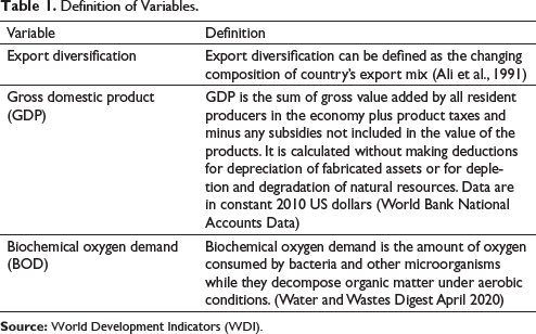
Definition of Variables.
The EKC literature uses the linear, quadratic and cubic specifications of the EKC model. Narayan and Narayan (2010), Sinha and Shahbaz (2018), Brown and McDonough (2016), and Shafik and Bandhopahhyay (1992) have used the linear specification of EKC modelling. However, linear modelling alone does not provide enough insight about how the pollutant varies with the income variable. Linear model approach evaluates the time derivative of the elasticity of the pollutant, which, at best, indicates that the relationship varies with time. Due to the shortcomings of linear modelling, we also estimate the quadratic specification. The quadratic model allows for the estimation of the first turning point in the curve and is the most commonly used specification in EKC literature. Studies, which discover an inverted U, proceed to detect if there is yet another turning point (or an N-shaped curve) and use the cubic model.
We articulate the quadratic form of the model.

In Equation (1), BOD is the dependent variable and GDP and the square of GDP2 are the explanatory variables, while export diversification (ED) is the additional variable.
Equation (1) can be rewritten as:

where lnBOD is the log of BOD, lnGDP is log of GDP, lnGDP2 is the log of GDP squared and lnED is the log of export diversification. ß0 is the intercept term; ß1 and ß2 are the parameters to be estimated; t is the time period; and ε is the error term.
Equation (2) can be used to test the following possibilities. If ß1 = ß2 = 0, then there is no pollution income relationship. If ß1 > 0 but ß2 = 0, then we obtain a monotonically increasing pollution income relationship. If ß1 < 0 but ß2 = 0, then we obtain a monotonically decreasing pollution income relationship. If there is a situation where ß1 < 0 but ß2 > 0, the pollution income relationship thus found is U-shaped. An inverted U-shaped pollution–income relationship or an EKC is found if ß1 > 0 but ß2 < 0 (De Bruyn et al., 1998).
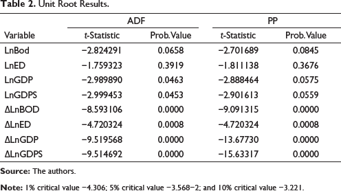
The stationarity properties of the variables are ascertained by employing the augmented Dickey–Fuller (ADF) and Philip–Perron (PP) tests, using the intercept and trend form in the unit root estimation (Phillips & Perron, 1988). Results of the ADF and PP are presented in Table 2. According to ADF, LnGDP and LnGDP square are stationary at level, while LnBOD and LnED are stationary at their first difference. The PP test results show that all the variables are stationary at their first difference. The variables are, therefore, integrated of the orders I(0) and I(1) according to the ADF results, and I(1) according to the PP results.
Unit Root Results.
Once stationarity properties among the variables are confirmed, we need to select the appropriate cointegration test to determine if there is a long-run relationship among the variables. The choice of the cointegration test depends on (a) the integration order of the variable, (b) the presence/absence of structural breaks in the time series data and (c) the number of structural breaks detected in the time series data. If the data series are integrated at I(0), then a simple regression model of OLS can be performed. If the data series are integrated at I(1) and I(0), in that case, the ARDL is applied. If all the data series are integrated at I(1), then the Engel–Granger cointegration test is employed if the model is bivariate, but in case of a multivariate model, the Johansen–Julius model is used. In case the series are I(2), the Toda and Yamamoto (1995) cointegration test can be performed. To determine the cointegration between the variables—BOD, GDP, square of GDP and export diversification—we perform the ARDL (Pesaran et al., 2001) and bounds cointegration test. The ARDL framework is based on the standard log-linear functional specification with the unrestricted error correction mechanism. The Akaike information criterion (AIC) has been used to select the lag order of the variables.
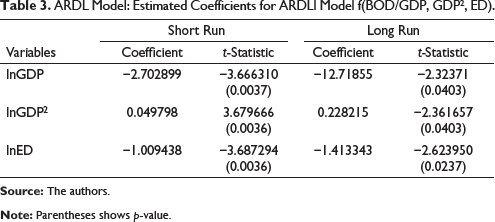
Table 3 shows the results of the ARDL test. Since the time series data has been transformed into their natural logarithms, the computed coefficients are equivalent to the elasticities. In the model f(BOD/GDP, GDP2, ED), BOD is significantly and negatively linked to GDP both in the short run and in the long run, whereas BOD is significantly and positively linked to GDP2 both in the short and the long run. This signifies that the pollution–income pathway is U-shaped in the long run. In this model, we have included export diversification as an additional variable. Results show that BOD is significantly and negatively related to export diversification in both the short run and the long run. Our findings reveal that an EKC does not exist for river water pollution in India for the period from 1986 to 2019 when we consider GDP, GDP2 and ED as explanatory and additional variables, respectively. However, we do find that river water pollution increases for an undiversified export basket. A higher value of the export diversification index indicates that the export basket is less diversified. Therefore, a negative sign for the coefficient of export diversification means that the export diversification positively affects BOD.
ARDL Model: Estimated Coefficients for ARDLl Model f(BOD/GDP, GDP2, ED).
The value of joint F-statistic is used to determine if there is a long-run relationship between BOD, GDP, GDP2 and ED. If the estimated F-statistic value is smaller than the lower critical bound, we cannot reject the null hypothesis of no cointegration. However, if the computed statistic value is greater than the upper critical bound, we reject the null hypothesis of no cointegration. However, if the estimated F-statistic value remains between the lower and upper bound critical values, the results remain inconclusive.
Table 4 shows the results of the bounds test. The F-statistic of the model f(BOD/GDP, GDP2 and ED) is 12.10155, which is greater than the upper critical bound (3.2). Therefore, it can be concluded that a strong long-run relationship exists between the variables BOD, GDP, GDP2 and ED.
Bounds Testing for Cointegration.
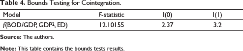
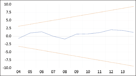
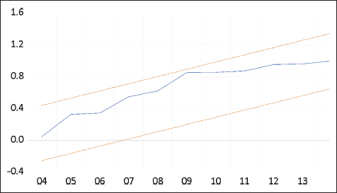
Table 5 shows the results of the error correction model. The negative and statistically significant coefficient estimate of the lagged error correction term (ECT) validates the presence of a long-run relationship among BOD, GDP, GDP2 and ED. For the model f(BOD/GDP, GDP2, ED), ECT (−1) has a coefficient of −0.714, suggesting the adjustment rate from disequilibrium to long-run equilibrium, or, in other words, approximately 71% of previous year’s disequilibrium is eliminated in the present year. Several diagnostic tests are conducted to check the robustness of the model. The goodness of fit of the specification (R-square) is approximately 92% for f(BOD/GDP, GDP2, ED). Higher values of R-square close to 1 are considered econometrically meaningful as they indicate the high explanatory power of the explanatory and additional variables with respect to the dependent variable. The model does not contain any serial correlation, as we cannot reject the null hypothesis of no serial correlation, and homoscedasticity, as the respective p-values of 0.2366 and 0.7741, far exceeds 0.05. The cumulative sum (CUSUM) and cumulative sum of squares (CUSUMSQ) of recursive residuals are performed to check the stability of the estimated model.
ECM Representation for ARDL Models.
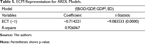
CUSUM and CUSUMSQ are presented in Figures 1 and 2. The estimated model and the short-run and long-run coefficients are stable over time as the residuals fall within the 5% significance boundaries.
This study attempted to investigate the EKC for river water pollution and export diversification in India over the period from 1986 to 2019. We applied the ADF–PP unit root test to determine the stationarity properties of the variables, followed by the ARDL cointegration test, as well as the bounds test, and, finally, estimated the elasticities using the error correction model.
Although a strong cointegration emerged between export diversification and water pollution, we did not find a conventional EKC pathway for the pollution–export diversification relationship for India over the period from 1986 to 2019.
Results of the quadratic model suggest that in the short run, BOD is significantly and negatively linked to GDP in both the short run and the long run, whereas BOD is significantly and positively linked to GDP2 in both the short run and the long run. This signifies that the pollution–income pathway is U shaped in the long run. Furthermore, BOD is significantly and negatively related to export diversification in both the short run and the long run. Our findings suggest that a conventional inverted U-shaped EKC does not hold for India over the period from 1986 to 2019 when GDP, square of GDP and export diversification are taken as explanatory and additional variables, respectively.
A strong cointegrating relationship was detected between export diversification and water pollution. Expectedly, this is because the Indian export mix is fairly concentrated. The top export industries—pharmaceuticals, organic chemicals, mineral fuels, textiles, nuclear reactors, electrical machinery and automobiles have dominated the export basket for nearly a decade now. All the aforementioned industries are classified as grossly polluting and among the ‘Red’ category in another classification, signifying the high pollution risk they pose. Evidence suggests that India’s commodity export basket is specialised or concentrated rather than diversified (Sangita, 2018). The coefficient for export diversification is negative and significant, implying that a higher diversification index leads to higher levels of BOD generation. (Since the Theil index is a concentration index, a higher index value means the export mix is concentrated or weakly diversified).
Although the approach for combating water pollution has to be multifaceted, some policy measures that can be considered for industrial water pollution abatement are as follows: redesigning market-based instruments or economic instruments, improved governance, people’s participation or a decentralised approach that builds pressure on industries to adopt cleaner technologies and horizontal collaboration among the industries with enormous proactive state support. Economics instruments use the market mechanism for pollution control. These include a broad range of policy tools such as pollution taxes, performance bonds, deposit–refund systems and marketable permits. Government’s use of fiscal instruments (other than the expenditure policy) in environmental policy is limited, even though the need to employ economic and fiscal policy instruments for the control of pollution and management of natural resources has gained recognition since the 1990s. Economic instruments can also be used as tools to subsidise technological improvements—grant-based subsidies (soft loans, hard currency below market rate, direct funding), financing-based subsidies (soft loans, green funds, public interest rate subsidies), tax-based subsidies (tax credits, tax exemptions, tax breaks, accelerated write offs) or risk-based subsides (subsidised insurance or reinsurance, liability caps, public sector indemnification) (Chakraborty & Mukhopadhyay, 2013).
A decentralised, bottom-up approach involving the local communities and civic societies is observed to be successful in controlling pollution in certain industrial clusters in India. Murty et al. in 1999 reported the results of a survey of a number of industrial estates and an all-India survey of large-scale water polluting factories, providing evidence of local community pressure, resulting in the industries complying with standards. This approach draws theoretical support from the Coase theorem (Coase, 1960). The Coase theorem states that the optimal level of pollution control could be realised through the bargaining between the polluters and the affected parties, given the initial property rights to either of the parties in the absence of transaction costs. Even with positive transaction costs, the bargaining could result in the reduction of externality though not to the optimum level. Recent empirical experiences show that the bargaining between the communities and polluters helped in reducing water pollution when the government was protecting the property rights to the environmental resource to the people.
For small and medium-sized enterprises, it is not economically feasible to have their own individual effluent treatment plants to comply with the command and control regulation. Collective action involving all the relevant parties for water pollution abatement (factories, affected parties and the government) is now seen as an institutional alternative for dealing with the problem of water pollution abatement in industrial estates, especially in India. A common effluent treatment plant (CETP) for an industrial estate confers the benefits of saving in costs to the factories and the reduction in damages to affected parties. There are many incentives for polluters, affected parties and the government for promoting collective action in industrial water pollution abatement (Murthy & Kumar, 2002).
Evidence from leather export powerhouses of Tamil Nadu and Uttar Pradesh suggests that the success of CETP depends on many factors. CETPs were successful in the Palar Valley of Tamil Nadu, which is an industrial cluster of tanneries but a failure for the tanneries’ cluster in Kanpur, Uttar Pradesh. The difference in the environmental performance of the two clusters can be attributed largely to the state of governance in the two states. Reasons for failure in Kanpur can be summarised as infrastructure deficit, weak institutions and enforcement, poor financial state of local state agencies, a failed partnership between tanners and the Uttar Pradesh Jal Nigam, governance failure and agencies fraught with endemic corruption, dominance of small and micro tanning firms and poor sense of environmental awareness and responsibility among the tanners.
The pollution crisis of tanneries in the Palar Valley of Tamil Nadu in the mid-1990s was overcome by collective action on the part of the tanners who had a shared goal of building and operating a CETP that met the pollution norms. Key elements of this joint endeavour were the proactive role of the state of Tamil Nadu, social linkages of the economic actors and organisational forms of the CETP. The state plays a decisive role in facilitating the implementation of collective solution (Kennedy, 1999).
Despite the slew of water pollution abatement policies and programmes, there is little success in cleaning India’s rivers. In India, air pollution norms are more effective than water pollution norms. The cornerstone water policy—the National River Conservation Plan—has brought little measurable benefit to rivers (Greenstone & Hanna, 2014). Our findings corroborate the need to aggressively combat industrial water pollution, in a way that policy design should be supported by radical institutional reforms. Also, the task of diversifying the export commodity basket will involve radical structural changes in the Indian economy like upgrading infrastructure and capital investment in the export sectors. Diversifying the commodity basket is not only a safeguard against changing global dynamics and economic vulnerabilities but also necessary for attaining the goal of sustainable development.
Footnotes
Acknowledgement
We gratefully acknowledge the comments provided by three anonymous reviewers. Their insightful suggestions helped in reshaping this paper to take it’s current and final form.
Declaration of Conflicting Interests
The authors declared no potential conflicts of interest with respect to the research, authorship and/or publication of this article.
Funding
The authors received no financial support for the research, authorship and/or publication of this article.