
Abstract
The present article attempts to decompose the COVID-19-induced shock to output and inflation of the Indian economy at the aggregate and disaggregate levels into demand and supply shocks for the period March 2020 to June 2020, using a structural Bayesian VAR model following Baumeister and Hamilton (2015, 2019). The results of the empirical analysis reveal that while the negative supply shocks dominate at the aggregate and disaggregate levels, their magnitude varies across industries. Demand shocks to output were positive in some industries like the manufacture of food products (10), textiles (13), chemicals and chemical products (20), and electrical equipment (27), but were outweighed by the negative supply shocks. In response to the COVID-19 shock the government announced the three pronged Atmanirbhar Bharat Abhiyan (ABA), which is a blend of demand management, supply management and structural policies. It not only promises to address the short-term distress caused to the industries due to the COVID-19 shock but also attempts to make them self-reliant and resilient to such shocks in future.
Introduction
The genesis of the COVID-19 shock to the Indian macro-economy lies in the lockdowns, layoffs, disruption in supply chains, and so on, which were the only solutions to tackling the medical emergency. The resultant economic fluctuations necessitated an urgent response from governments to tackle the combined range of effects (Bekaert et al., 2020), which can be termed shocks to the economy. An economic shock is an unexpected exogenous disturbance that has a significant (usually adverse) impact on macro-economic variables (Kar & Bhattacharya, 2011). Economists initially debated whether the COVID-19 shock could be treated as a demand shock caused by rising unemployment and falling incomes and purchasing power among the people, or a supply shock resulting from a breakdown in supply chains, the shutting down of industries, and so on. (Bekaert et al., 2020; del Rio-Chanona et al., 2020). Triggs and Kharas (2020), were of the opinion that the COVID-19 shock was not just a demand and supply shock but also a financial shock. Eventually, however, most economists concurred that COVID-19 was a real shock to the economy with supply and demand elements (Caballero & Simsek, 2020). Guerrieri et al. (2020) showed how the supply shocks generated by COVID-19 would further generate aggregate demand shocks far larger than the original shock. Second-round effect of the demand and supply shocks from COVID-19 were also expounded on in India’s Economic Survey 2020–21 (Ministry of Finance). Thus, to address COVID-19-generated downturns to the economy it is important to decompose the COVID-19 shock into its demand and supply components at the aggregate and disaggregate levels, and to prescribe policy initiatives to help generate a V-shaped recovery (as against a K-shaped recovery which is not desirable).
The impact of the strict lockdown 1 on India’s economy was massive, and caused the growth rate of quarterly GDP to fall to –23.9 per cent in the first quarter of 2020. Industrial output also suffered a major jolt (Figure 1).
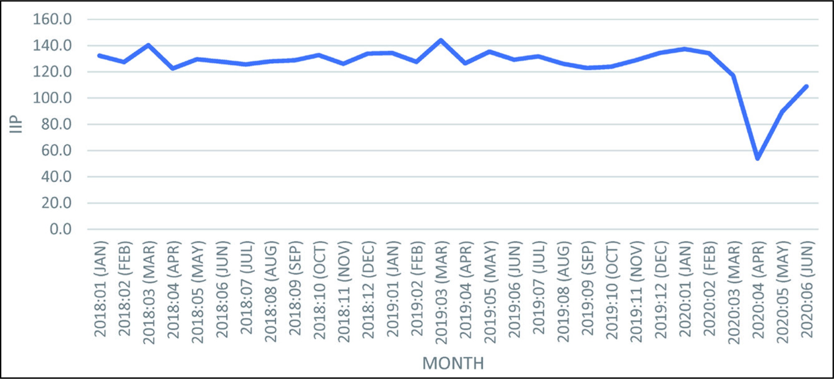
The Index of Industrial Production (IIP), which was at 134.2 in February 2020, fell to117.2 in March 2020 after an 8-day complete lockdown. In April it fell to 54 after which it started improving from 89.5 in May to 108.9 in June. It is important note that even if the IIP depicts a V-shaped recovery, many indirect effects of the COVID-19 shock may, eventually exacerbate the long-term impacts, giving rise to a K-shaped recovery.
The present study takes up the decomposition of the COVID-19-induced shock in the output and inflation space, using a Bayesian vector autoregressive model, to look at the demand and supply components at the aggregate and disaggregate levels. The article does not attempt to give any policy prescriptions to remedy the impact of shocks at any level.
The empirical results highlight that the peak of the shock to output for most of the industries considered occurred in April 2020; and that the shock to inflation it was felt in May 2020. The magnitude of the shock varied across industries and it was the negative supply shock that was the major cause of the decline in output. The demand shock was positive for some industries, but its magnitude was negligible and completely overpowered by the negative supply shock. The response of price inflation to the shock was muted, even though some goods became unavailable (Jaravel & O’Connell, 2020). The rest of the article is organised as follows: In Section 2, the literature on the impact and decomposition of the COVID-19 shock have been reviewed. The empirical methodology for this study is covered in Section 3. The results of the empirical analysis and the government’s policy response for the industry are discussed in Section 4, and Section 5 concludes.
The scale and nature of the COVID-19 shock has been unlike anything that has been faced by nations in the recent past (Tenreyro, 2020). The present study delves into the analysis and decomposition of the economic shock kindled by the COVID-19 pandemic.
Studies on Shocks Generated by the COVID-19 Pandemic
The international literature on COVID-19-manifested economic shocks can be broadly classified into studies focussing on supply shocks due to the COVID-19 pandemic (Bekaert et al., 2020; del Rio-Chanona et al., 2020; Fornaro & Wolf, 2020; Hiroyasu & Yasuyuki, 2020); studies focussing on demand shocks due to COVID-19 pandemic; and studies relating to the rare dynamics of both supply and demand shocks (Brinca et al., 2020; Caballero & Simsek, 2020; Guerrieri et al., 2020). These can further be classified as studies conducted at an aggregate level and those pertaining to the disaggregate or firm-level analysis (Brinca et al., 2020; Caballero & Simsek, 2020; Guerrieri et al., 2020). Some studies attempt to identify the demand and supply effects on prices and output either at the aggregate or the disaggregate level (Balleer et al., 2020; Bekaert et al., 2020), while others focussed on labour markets (Brinca et al., 2020).
While acknowledging that the Indian economy was already slowing down in the pre-pandemic period, most economists have been seriously concerned about the additional jolt suffered from the pandemic (Dev & Sengupta, 2020). However, studies analysing the demand and supply impact of COVID-19 have been descriptive and theoretical (Nath, 2020; Samaddar et al., 2020). Macroeconomic uncertainty associated with the COVID-19 shock was analysed by Das (2020). Estupinan et al. (2020), attempted to estimate first-order supply shocks through labour supply reductions associated with the economic pause due to the pandemic.
Some studies made a preliminary assessment of the sectoral impact of the COVID-19 shock using descriptive analysis (Rakshit & Basistha, 2020; Singh & Neog, 2020). Sahoo and Ashwini (2020) attempted to empirically forecast the impact of the COVID-19 shock on growth, manufacturing, trade and the MSME sector under three case scenarios. Deshmukh and Haleem (2020) prescribed the adoption of a mix of conventional manufacturing, special purpose machines (automated) and industry, to make the manufacturing sector resilient to such shocks. Seetharaman (2020) proposed a shift in the business models of labour-intensive manufacturing firms to digital replacements for their processes, and delivery of products or services with minimal physical contact.
Review of the Methodologies Used to Decompose the Shocks
Structural and calibrated models were used by some studies to identify the demand and supply shocks (Baqaee & Farhi, 2020; Fornaro & Wolf, 2020; Guerrieri et al., 2020). Empirical techniques such as the non-Gaussian features of macro-economic forecasts, Bayesian VAR models using sign restrictions and informative priors for identification of the shocks, were used for this (Balleer et al., 2020; Bekaert et al., 2020; Brinca et al., 2020). In a Bayesian estimation the most important challenge lies in specifying a prior distribution which, after applying the Bayes theorem, gives the posterior distribution of the parameters of interest. The choice of a prior is an extremely sensitive issue (Ocampo & Rodríguez, 2012), and as a result, for a very long time, the Bayesian VAR models were estimated using the non-informative priors specified by Jeffreys (1961). Subsequently, the Minnesota prior of Litterman became extremely popular in Bayesian VAR models. Kilian and Murphy (2012), while estimating demand and supply shocks to oil prices, made prior specification by combining sign restrictions with additional information on the bounds for supply elasticity, that is, they used a more informative prior. Baumeister and Hamilton (2015, 2019) revisited the oil demand and supply shock of the Kilian (2009) and Kilian and Murphy (2012) approach, and attempted to further improve prior information by proposing specific values for the parameters of the structural coefficient matrix derived from previous studies. Brinca et al. (2020) applied the Baumeister and Hamilton (2015, 2019) methodology to decompose the shock from COVID-19 to labour markets in the U.S.
From the review of international studies on the impact of the COVID-19 pandemic on economies, it is clear that for framing targeted policies it is important to first understand the nature of the COVID-19 shock and decompose it into its components (i.e., the demand component of the shock and the supply component). To the best of the author’s understanding no studies have so far attempted to empirically decompose the COVID-19 shocks on output and prices in India into the demand and supply components, either at the macro level or at the disaggregate level. The present study tries to fill this gap by empirically decomposing the economic shock caused due to COVID-19 into demand shocks and supply shocks using the Baumeister and Hamilton (2015, 2019) Bayesian VAR techniques for 20 industries from the manufacturing sector and also at the aggregate level.
Methodology
Variables and Data Sources
Since the data on GDP (output) for India is available quarterly and not monthly, the general IIP has been used as a proxy for aggregate output. The consumer price index combined (CPIC) has been used to estimate aggregate inflation, which is the official measure of inflation in India. The IIP of industries with NIC 2008 classification codes 10 to 31 (except 19) have been used. (These industries have been used because of the availability of their price and output data.)
Empirical Methodology
Vector autoregressive models (VARs) are the most popular tools for estimating macro econometric models. The structural parameters and shocks can be derived from the reduced-form VAR only if some identifying restrictions are applied to the structural parameters. The present article follows the Baumeister and Hamilton (2015, 2019) methodology, which improves on the Uhlig (2005) method of applying sign restrictions and more informative priors in a Bayesian format to identify the structural shocks.
Data For the Variables Used

Data For the Variables Used
Consider the following dynamic structural model:
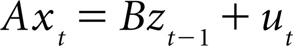
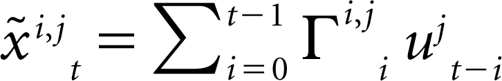
Where xt is a 2x1 vector of observed variables (output gap and inflation in the present case); A is a 2x2 matrix summarising the contemporaneous structural relations of the variables in xt; zt–1 is the kx1 vector (with k = mn+1), containing a constant and m lags of xt, such that zt–1 = (xt–1’, xt–2 ’… xt–m’, 1) and ut is a n x1 vector of structural disturbances. The variance of the matrix ut is assumed to be diagonal and denoted as D.
In its expanded form, if m = 1, equation (1) can be written as
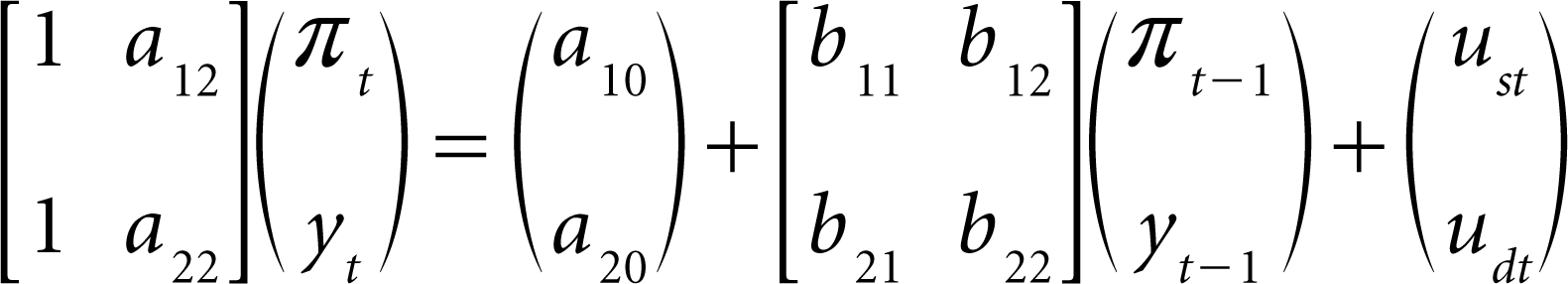
Where, a12 and a22 are the structural parameters of the equation for inflation and can be termed the aggregate elasticity of supply and aggregate elasticity of demand of inflation, respectively. Similar equations can also be derived for output. For estimation, equation (1) must be converted into a reduced-form equation by multiplying it by the inverse of matrix A, so that the contemporaneous impact of the elements of xt are done away with. However, for identification of the structural parameters from the reduced-form equations, restriction must be applied to the matrix A. The present study follows Baumeister and Hamilton (2019), which augments the sign restriction of Uhlig (2005), with more informative priors for identification of the structural parameters. The empirical estimation using Bayesian techniques requires the specification of priors of:
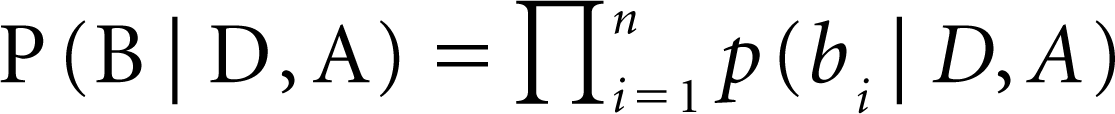
The prior information of the parameters in the current context p(A,D,B) gives the joint distribution of A, D and B, which is the product of the respective distribution. The posterior distribution (equation 5) derived after applying Bayes’ theorem to the joint prior distribution, summarises the researcher’s uncertainty about parameters conditional on having observed the sample YT.

Baumeister and Hamilton (2015, 2019) provide the algorithm which can be used to generate N different draws from the joint posterior distribution given in equation (5).
‘Historical decomposition allows us to make a statement on what has actually happened to the series in the sample period, in terms of the recovered values for the structural shocks’ (Ocampo & Rodríguez, 2012). Thus, it is possible for us to examine the relative effects of each shock on the variables in the VAR system because historical decompositions give the history of the shock on the variables. The residuals et derived from the reduced-form equation can be used to derive the structural shocks as follows:
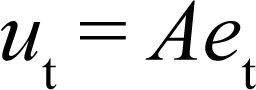
The vector moving average representation of the VAR model can be written as
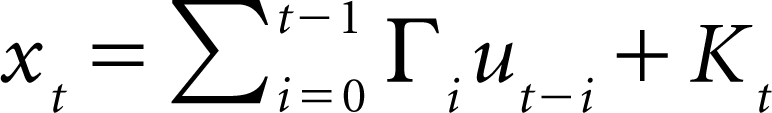
In equation (1b) the variables in xt depend upon the effects of all shocks that are realised previous to the sample, which are captured by the initial values (denoted by Kt) of the variables in the VAR system. As t increases, Kt tends to the mean value of the elements of the VAR model. The historical decompositions are made over the auxiliary variable
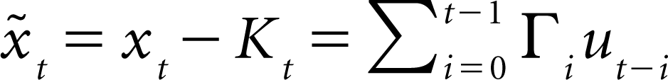
such that the historical decomposition of the ith variable to the jth shock is given by:
Baumeister and Hamilton (2015, 2019) provide the algorithm to estimate the historical decompositions and their 95 per cent credible intervals, which have been incorporated in the BHSBVAR package of Richardson (2020).
Sign Restrictions and Prior Specifications
The prior for the structural parameters of matrix A2, variance covariance matrix D of the structural parameters and the lagged parameters of the VAR system are specified as follows:
Prior for the Elements of Matrix A
To specify the prior for a given parameter, researchers normally bank on past studies. Structural parameters find a proxy in the slope of the aggregate demand and aggregate supply curves estimated at the aggregate level for the country. We follow Goyal and Kumar (2018), who provide a range of slope parameters for the aggregate demand and supply curves, depending on the habit persistence parameter, 3 in a DSGE framework. These parameters differ significantly for India, compared to other nations, such that at a given level of habit persistence, the steady-state-level of the slope of the aggregate demand curve is as high as –98.57, and the slope of the aggregate supply curve is 1.19. Thus, the sign of the elasticity of aggregate demand in the current study is assumed to be negative, and that of aggregate supply is assumed to be positive. It is assumed that the elasticity of aggregate demand (a22) has a t distribution, with a location parameter equal to –23.1 and scale parameter equal to 0.6 at 3 degrees of freedom, so that we can assume a 90 per cent probability on a22 ϵ [–23, –23.5]. Similarly, the aggregate supply elasticity (a12), also has a t distribution with a location parameter equal to 1.5 and scale parameter equal to 0.6 (following Baumeister & Hamilton, 2015), at 3 degrees of freedom, so that we can place a 90 per cent probability on a12 ϵ [1.19, 2]. The range of elasticity begins at 1.19 (following Goyal & Kumar, 2018), however the upper value was chosen keeping in mind the wide variation in the elasticity of supply derived by studies which estimate the aggregate supply curve of India (Salunkhe & Patnaik, 2019).
At the disaggregate level, to the best of the author’s knowledge there are no studies on India which can help set the location parameter of the priors of the elasticities of supply and demand. As a result, the median values of the aggregate elasticities of demand and supply derived from the Bayesian estimation of the same for aggregate inflation and output (in the present study) were used as location parameters at the disaggregate level. While the location parameter of the aggregate elasticity of demand fitted the sectoral data approximately, the elasticity of supply varied across sectors. Subsequently, the location parameter for the elasticity of supply at the sectoral level was determined using the median value of the annual elasticity of supply of that sector for the sample period, such that it varied within the range, a12 ϵ [3, 30]. The distribution and scale parameters of a22 and a12 were assumed to be the same as at the aggregate level, across all the sectors.
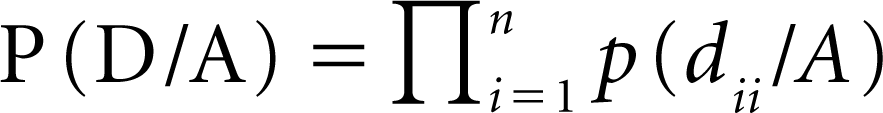
Conditional Prior p(D/A) and p(B/D, A)
Following Baumeister and Hamilton (2019) we assume that the reciprocals of the elements of the diagonal matrix D follow a gamma distribution with shape parameter κi and scale parameter τi. Following Brinca et al. (2020), we set κi equal to 2 and the scale parameter τi in such a manner that the prior mean κi/τi matches the precision of structural shocks after orthogonalization of the univariate autoregressions with the desired number of lags under A. Which means that, τi = κi
Elasticities of Demand and Supply (Aggregate and Sectoral)
Having estimated the Bayesian VAR model using the Baumeister and Hamilton (2019) methodology, we report the median values of the elasticities of demand and supply, and the plot of the historical decomposition of demand and supply shocks to which aggregate output and aggregate inflation were subject in the 12 months, that is, May 2019 to June 2020.
The posterior distributions of the structural parameters of all the estimated VAR models have been reported in Appendix 1. In most cases the posterior distribution (which is shown by the blue plots) is in sync with the prior distribution. This means that the prior distributions were informative and fitted the data well. The median values of the elasticities of aggregate demand and supply have been plotted in Figure 2.
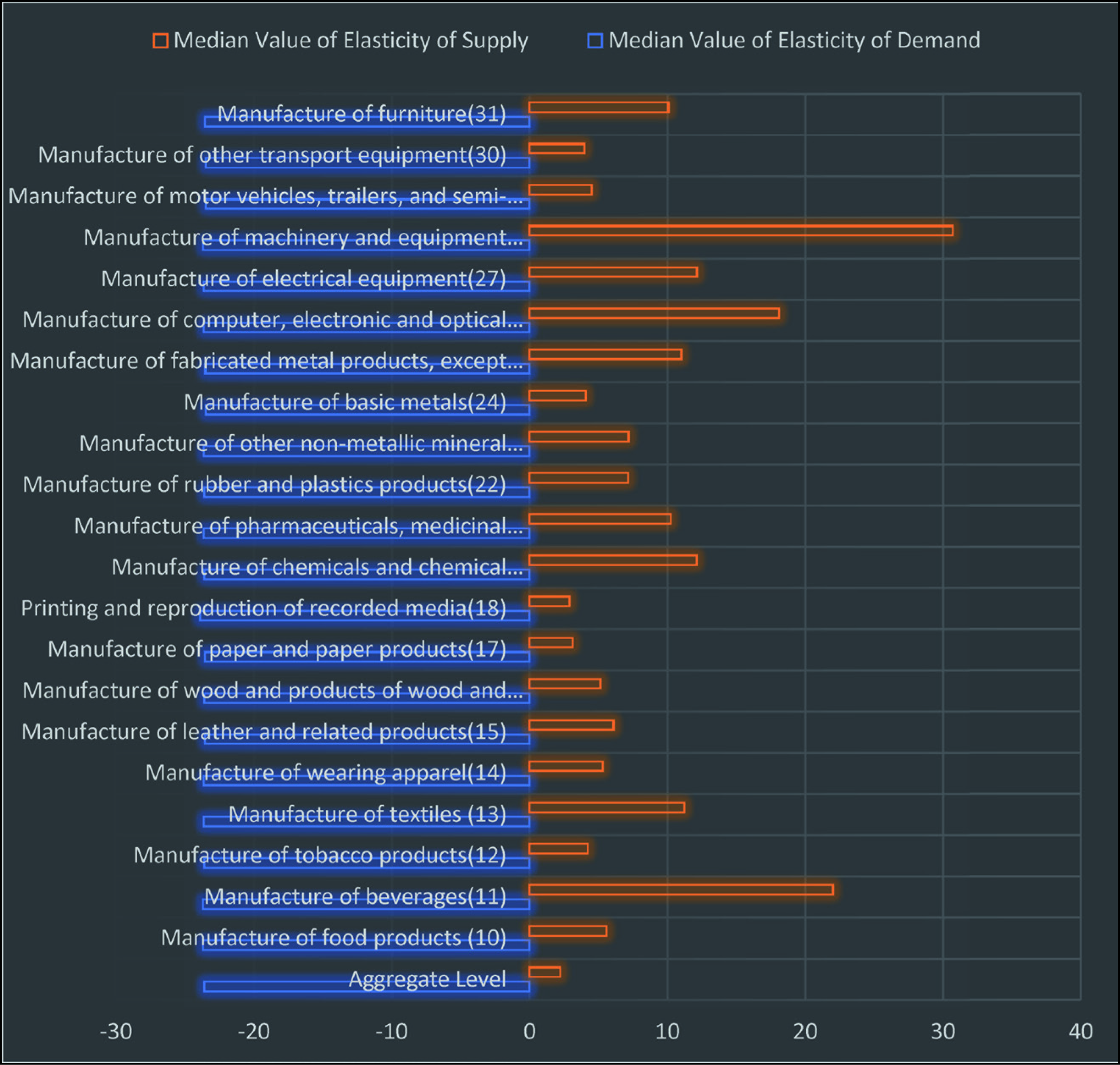
The median value of the elasticity of aggregate demand is –23.58 and that of aggregate supply is 2.22. From these results it can be inferred that the aggregate demand curve is downward sloping and the aggregate supply curve is upward sloping. Also, the aggregate demand curve is more elastic than the aggregate supply curve. It is important to note that these estimated elasticities though not equal are close to the results of Goyal and Kumar (2018). At the sectoral level, the elasticity of sectoral demand is around the elasticity of aggregate demand, however the elasticity of sectoral supply fluctuates greatly across sectors. The range of the elasticity of supply across the 20 industries is 2–30, with the industry engaged in the manufacture of machinery and equipment (28) having the highest elasticity of supply.
Historical Decomposition of Shocks to Aggregate Output and Prices (IIP General and CPI-C)
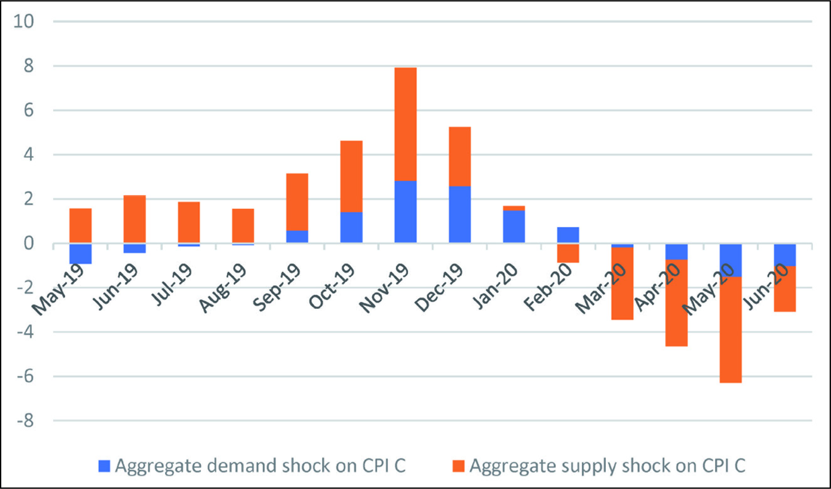
The historical decomposition of the shocks to the IIP and CPI-C inflation for the period of May 2019 to June 2020 have been depicted in Figures 3 and 4, and the historical decompositions of the same for the entire sample period can be seen in Appendix 2. In all the figures depicting the historical decompositions, the orange bars represent supply shocks and the blue bars the demand shocks. The sum of these bars implies the percentage change in the growth rate of output or inflation from its historical average; the size of the orange bar relative to the blue bar shows how important the supply shocks are relative to the demand shocks for output/inflation (Brinca et al., 2020).
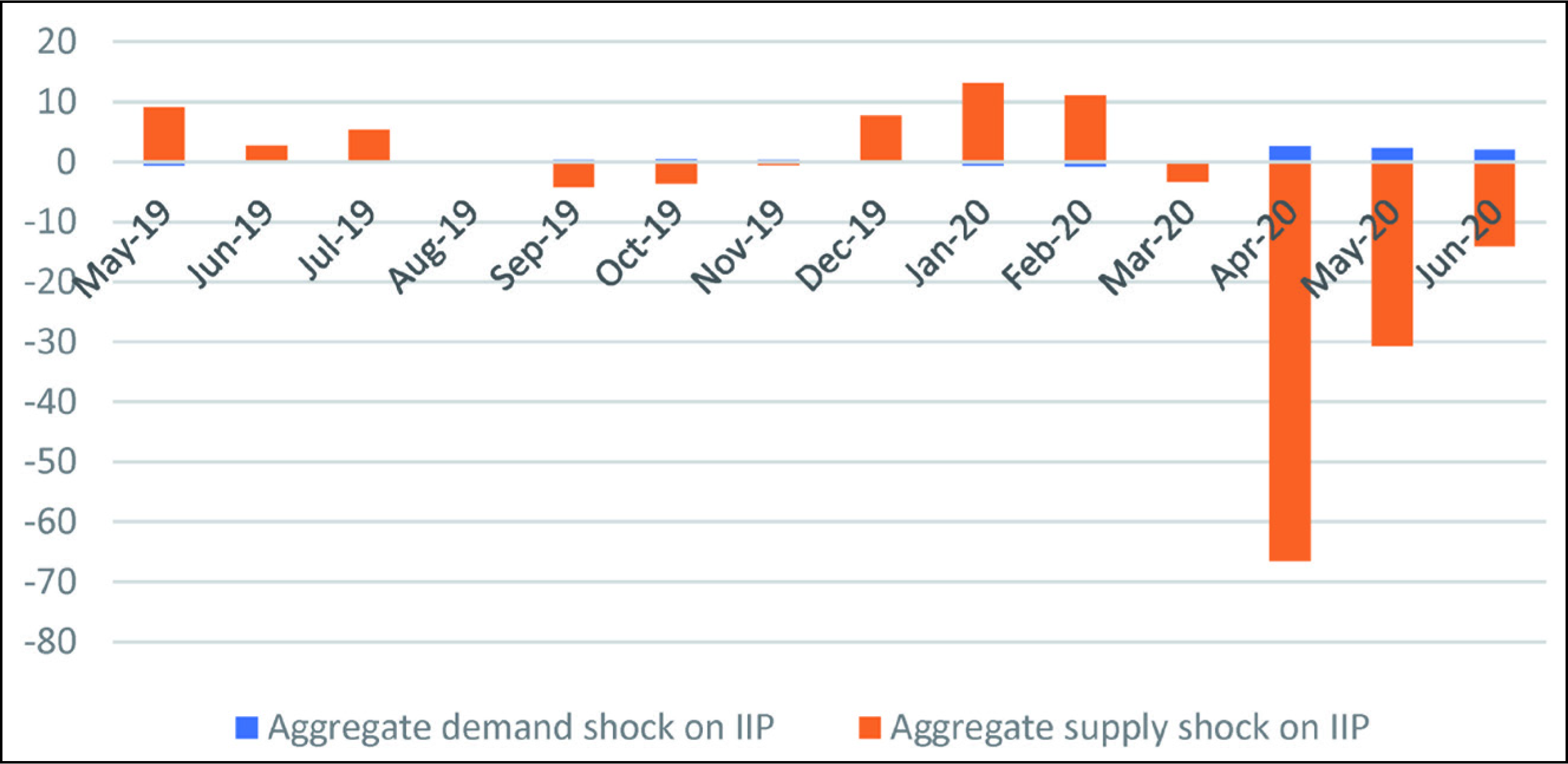
It can be inferred (from Figure 3) that prior to the COVID-19 shock period, demand and supply shocks to IIP oscillated within a narrow band of –4 to 12 per cent and, barring the months of September and October 2019, these shocks were mostly positive. However, from March 2020 onward, the supply shocks became negative and in April 2020 the maximum impact occurred when the supply shock caused a 66.4 per cent fall in the growth rate of IIP compared to its long-term average value. In May and June 2020, though the negative supply shock continued to influence the IIP, its magnitude was lower than in the previous months (–30.6 per cent in May 2020 and –14.29 per cent in June 2020).
The magnitude of negative supply shocks started falling in May and June 2020, but it was still extremely high compared to the average supply shock during the entire time sample under consideration. The demand shock to IIP was positive in all three months, however, the magnitude of the positive demand shock was extremely small compared to the negative supply shock (2.5 per cent in April, 2.3 per cent in May and 2.1 per cent in June 2020); and the negative supply shock over-shadowed the positive demand shock. It is also evident that the peak of the negative shock to IIP was felt in the month of April 2020 and gradually started receding, though it continued to be negative.
CPI-C inflation, however, responded differently to the COVID-19 shock, both in terms of magnitude as well as nature of the shock. The peak of the shock was felt in May 2020, after which its magnitude started declining. The magnitude of the negative supply shock in April and May 2020 was –3.9 per cent and –4.78 per cent, respectively, and of the negative demand shock in April and May 2020 was –0.74 per cent and –1.52 per cent, respectively. It is thus clear that the magnitude of the negative supply shock was higher for the IIP compared to CPI-C inflation; and that the demand shock was negative in the case of CPI-C inflation and positive for the IIP during the same period.
The historical decomposition of shocks to the 20 industries has been summarised in Tables 2 and 3. In Table 2, the last column gives the total number of people employed in these industries, indicating the volume of people impacted in each industry.
Industry-Wise Historical Decomposition of Supply Shock to WPI and IIP (March 2020 to June 2020)
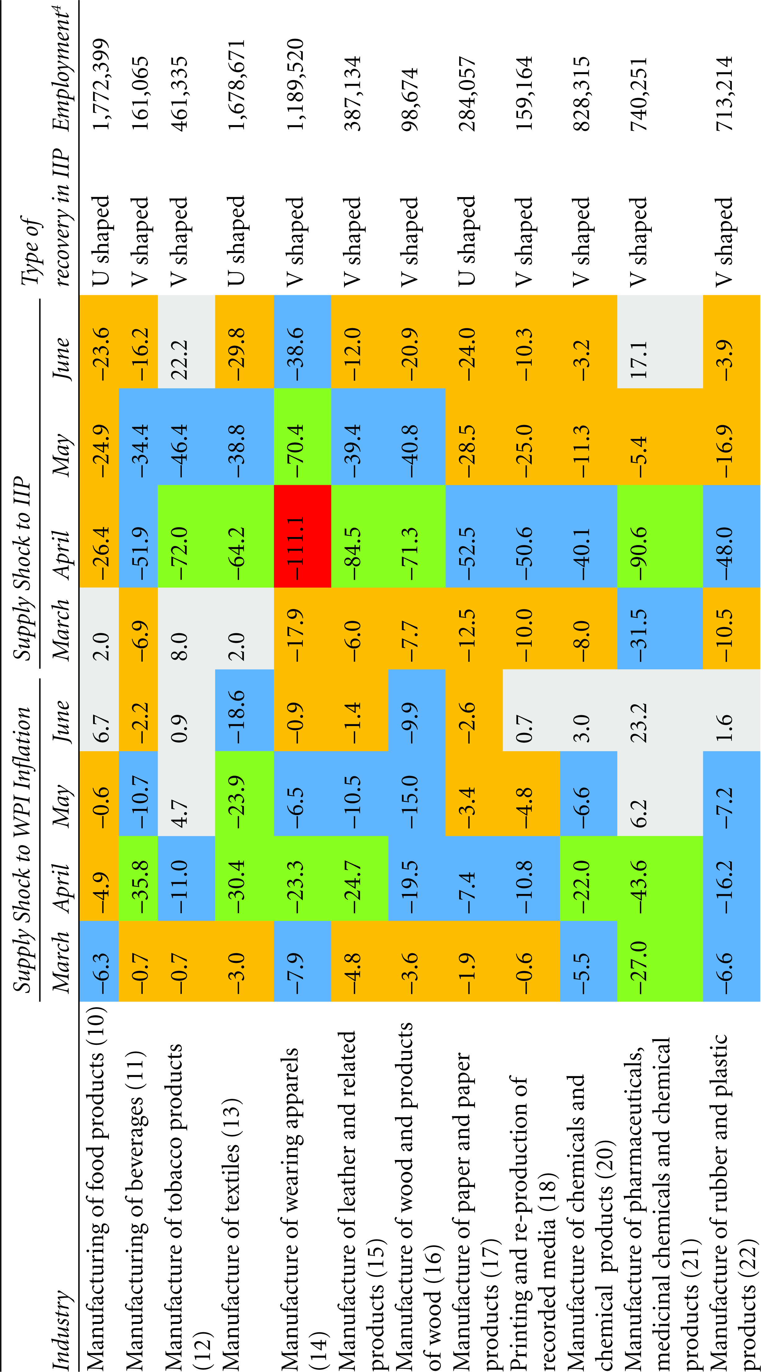
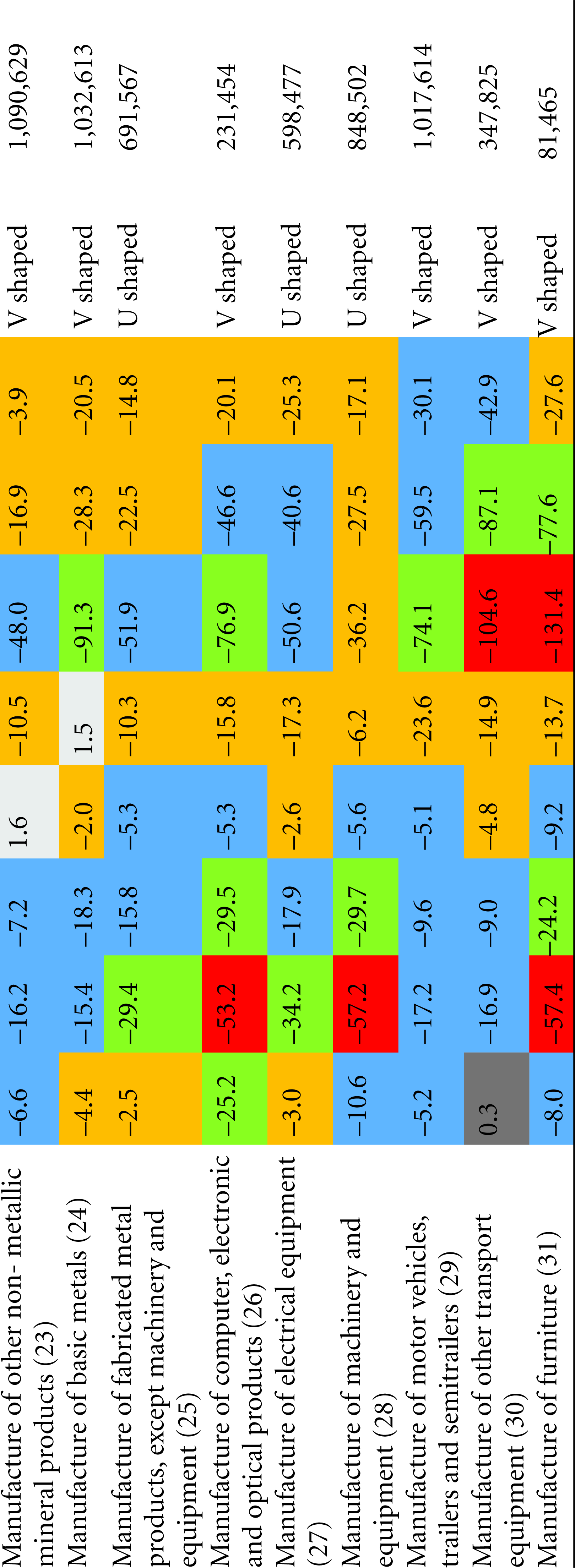
Industry-Wise Historical Decomposition of Supply Shock to WPI and IIP (March 2020 to June 2020)
Grey: positive supply shock; Red: most severe shock—a negative supply shock above –100 per cent to the IIP and over –50 per cent to the WPI; Green: severe shock—a negative supply shock of between –60 and –100 per cent to the IIP, and between –20 to –50 per cent to the WPI; Blue: moderate shock—a negative supply shock between –30 and –60 per cent to the IIP and between –5 and –20 per cent to the WPI; and Yellow: mild shock—a negative supply shock between 0 and –30 per cent to the IIP and between 0 and –5 per cent to the WPI.
The following observations emerge:
The IIP was dealt the most severe supply shocks (colour code red) in April 2020 in the following industries: manufacture of furniture (30); manufacture of other transport equipment (31); and manufacture of apparels (14). The WPI in the following industries experienced the most severe supply shocks: manufacture of computers, electronic and optical products (26); manufacture of machinery and equipment (28); and manufacture of furniture (31). Severe supply shocks (green) were experienced by: the IIP of industries engaged in manufacture of tobacco products (12); manufacture of textile (13); manufacture of leather and related products (15); manufacture of wood and wood products (16); manufacture of pharmaceutical, medicinal, chemical and botanical products (21); manufacture of basic metals (24); manufacture of computer, electronic and optical products (26); and manufacture of motor vehicles, trailers and semi-trailers (29); and the WPI of industries manufacturing beverages (11); manufacturing textile (13); manufacturing wearing apparel (14); manufacturing leather and related products (15); manufacturing chemicals and chemical products (20); manufacturing pharmaceuticals (21); manufacturing fabricated metal products (25); and manufacturing electrical equipment (27). A moderate supply shock (colour code blue) was felt by the IIP of industries engaged in the manufacture of beverages (11); manufacture of paper and paper products (17); printing and reproduction of recorded media (18); manufacture of rubber and plastic products (22); manufacture of other non-metallic mineral products (23); manufacture of fabricated metal products except machinery and equipment (25); manufacture of electrical equipment (27); and the WPI of industries manufacturing food products (10); manufacturing tobacco products (12); manufacturing paper and its products (17); printing and reproduction of recorded media (18); manufacturing rubber and plastic products (22); manufacturing other non-metallic mineral products (23); manufacturing basic metals (24); manufacturing motor vehicle, trailers and semi-trailers (29); and manufacturing other transport equipment (30). The peak of the supply shock to the IIP of all industries under study was felt in the month of April 2020 and after which the magnitude of the negative supply shock started falling. In the month of June 2020 two industries namely, manufacture of tobacco products (12) and manufacture of pharmaceutical, medicinal chemical and botanical products (21) registered positive supply shocks.
Industry-Wise Historical Decomposition of Demand Shock to WPI inflation and IIP (March 2020 to June 2020)
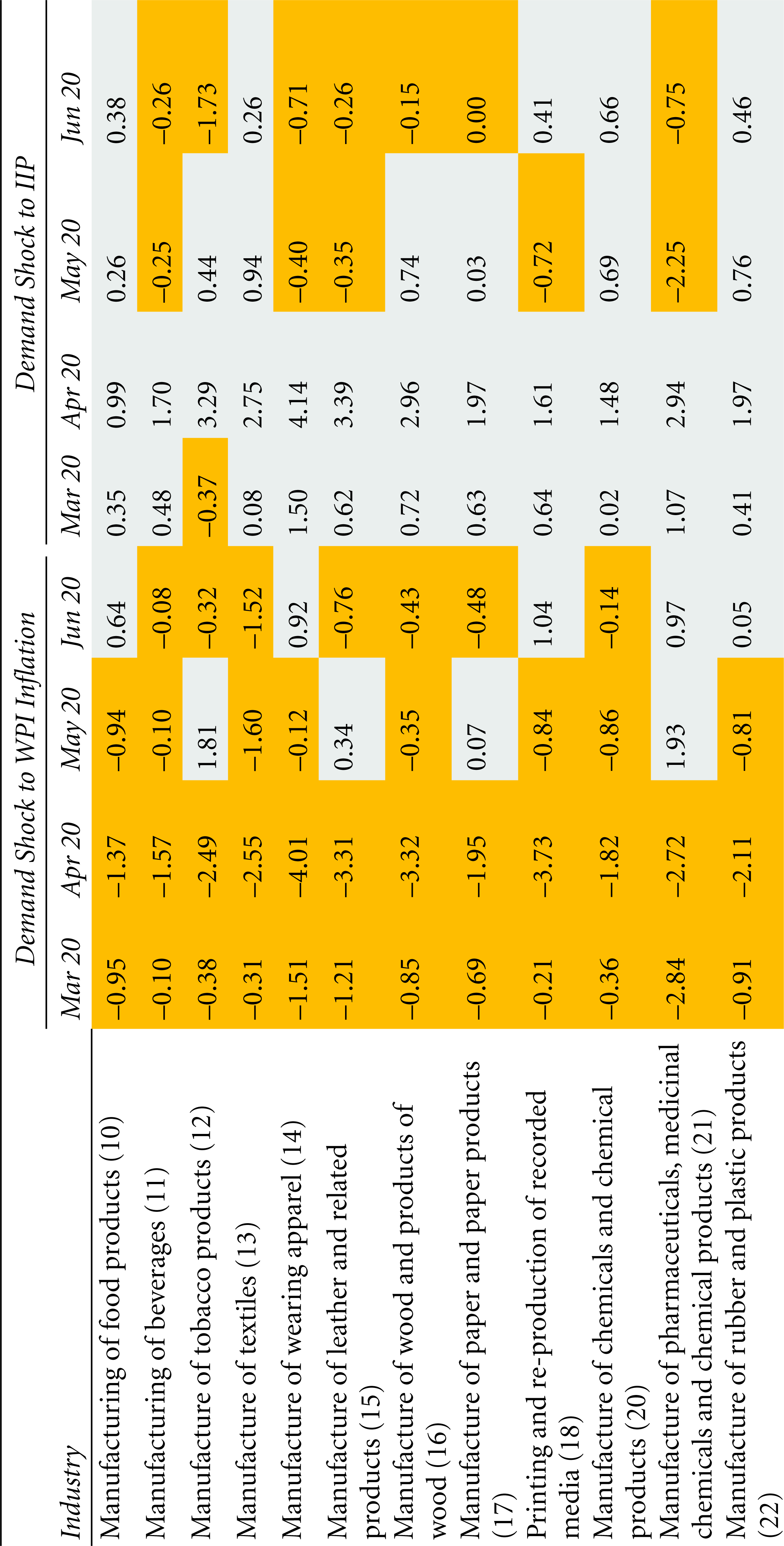
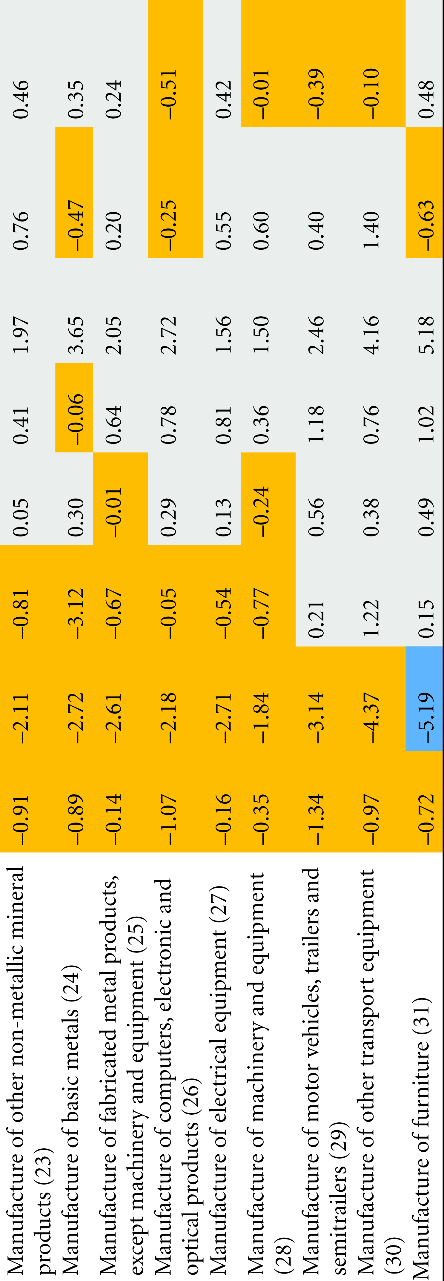
The demand shock to the IIP was mostly positive and marginal, except for a few industries, and was eventually subdued by the negative supply shock. The magnitude of the negative supply shock to WPI inflation was less than the magnitude of the negative supply shock to the IIP. The peak of the shock was felt by the IIP in May 2020, and it remained largely negative over April to June 2020. The WPI of most industries under consideration was subject to a negative demand shock in April and May 2020. However, in June 2020 the WPI of some industries like manufacture of food products (10); manufacture of apparel (14); painting and recorded media (18); manufacture of pharmaceuticals (21), and so on, were subject to a marginal positive demand shock. The recovery of most of the industries appear to be a V shaped. Bulk of the industries which suffered most severe to moderate supply shock are either labour intensive or depend on exported inputs (e.g., The Indian Pharmaceutical industry, manufacture of automobiles, etc., which started facing negative supply shock from the month of March 2020, due to lockdown in China in February 2020 and the resultant shortage of exported inputs)
As the impact of the COVID-19 shock unfolded the central government of India and the RBI announced monetary, fiscal and sector-specific policy measures under an umbrella scheme, the Atmanirbhar Bharat Abhiyan (ABA), which accounted for 10 per cent of the country’s GDP. The three-pronged ABA (which was a blend of demand and supply management and structural reforms) was announced in three phases, 1, 2 and 3. Some of the policy measures targeting the industrial/manufacturing sector are:
The Micro, Small and Medium Enterprises (MSMEs), which contribute 40–45 per cent of the manufacturing output in the country. In the ABA 1 the government introduced a Rs 200 million package called the Emergency Credit Line Guarantee Scheme 1 (ECLGS-1), to address the working capital needs, operational liabilities and restart business of the MSMES impacted due the COVID-19 crisis. The scheme also supported the lending institutions by giving 100 per cent guarantee for losses suffered by them due to non-repayment of funds by MSMEs and other small businesses. Thus, the scheme was fool proof as regards reaching out to the distressed MSMEs, and also making them resilient to such shocks in future.
In the ECLGS 2 scheme which was announced in November 2020, the existing corpus of ECLGS 1.0 was extended to provide 100 per cent guaranteed collateral free additional credit to entities in 26 stressed sectors (identified by the Kamath Committee, of RBI (2020)) as on 29.2.2020. Out of these 26 sectors more than 10 sectors (Textile, Chemicals, Sugar, Automobile manufacturing, plastic manufacturing, building materials, auto components, pharmaceutical manufacturing, consumer durables, etc.) belonged to the manufacturing sector. It can be seen from Table 2 that these were the sectors that were worst affected by the COVID-19 shock.
In order to expand the ambit of the ECLGs the definition of what constitutes an MSME enterprise has also been expanded. Loans to these enterprises will be granted for four years and the principal repayment will start after a 12 month moratorium.
The Production Linked Incentive (PLI) scheme which was announced in April 2020 for Large scale electronic manufacturing firms, and later expanded to 10 more sectors (which comprises of many industries covered in Table 2) aims to make the manufacturing sector self-reliant, by protecting identified products areas, discouraging imports, and promoting exports by the beneficiaries of the scheme. This scheme thus attempts to reduce the reliance of the manufacturing sector on import and therefore immunizes it from the international supply chains.
Conclusion
From the result of empirical analysis, it can be concluded that the immediate impact of the economic pause and breakdown of supply chains (domestic as well as international) as a result of COVID-19 was massive supply shocks to the output and price inflation of India in April 2020, at the macro and industry levels. Subsequently, some industries and the macro economy started being subjected to negative demand shocks, in addition to the negative supply shock which was relatively milder in May and June 2020. Demand shocks to output were positive in some industries like the manufacture of food products (10), textiles (13), chemicals and chemical products (20), and electrical equipment (27). The magnitude of the demand and supply shocks varied across industries, and supply was inelastic in many industries. Though the IIP of many industries started depicting a V-shaped recovery from the supply shocks by June 2020, policy intervention became necessary, not only to mitigate the impact of the lockdown but also to immunise industries from such shocks in future. The government attempted to deal with the short-term credit needs of the stressed industries and to make them self-reliant and resilient to such shocks through its ABA policy. The efficacy of the ABA policy in addressing the economic crisis will unfold only over a period of time. The present study covered only the peak period of the first wave of the COVID19 pandemic. The economic impact of the second wave of the pandemic, when lockdowns were localised and minimum disruptions were caused to the regular functioning of these industries, can be explored through further research.
Footnotes
Declaration of Conflicting Interests
The author declared no potential conflicts of interest with respect to the research, authorship and/or publication of this article.
Funding
The author received no financial support for the research, authorship and/or publication of this article.
Appendix 1
Appendix 2