
Abstract
Background
Living conditions are becoming challenging day by day. Mental stress on individuals is increasing due to multiple reasons. As mental stress is a major cause of mental illness, it must be detected at the earliest to prevent serious conditions such as depression and anxiety.
Purpose: The focus of this study is to detect the exact location of the source which causes such damage. In this article, we analyse the mental conditions of subjects under a workload of performing mental arithmetic calculations for various frequency bands and plot the topography to understand the areas of active potentials.
Methods: We propose a Novel Cluster Ensemble Verifier (CLEVER) algorithm, which combines two different techniques: clustering and source localisation. The proposed algorithm is highly efficient in identifying the exact location of the source. It is seen that the topographic plots of the independent component analysis (ICA), which has the maximum percentage of relative variance, correlates to the cluster generated. We are able to give the percentage-wise contribution of every component which is responsible for brain source activation with less time complexity.
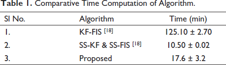
Results: Out of 72 subjects, in 67 subjects, 299 out of 433 components originate from the occipital and parietal areas of the brain with a maximum power of 43.5 µv2. As an example, the relative variance of one component is found to be contributing up to 74.03% to source activations. Clusters show similarity across the subjects in the parietal and occipital areas of the brain. The dataset used for experimentation is EEGMAT from Physionet’s repository. The computation time for the algorithms is 17.6 ± 3.2 minutes.
Conclusion
Findings show that during mental arithmetic calculations, both occipital and parietal areas of the brain are involved. As the data is acquired by orally mentioning the mathematical problem, subjects tend to visualise the numbers while finding the solution, which is reflected in the occipital area of the brain. CLEVER algorithm verifies the origin of the activity in the occipital and parietal areas of the brain.
Introduction
EEG is the safest and most non-invasive technique to acquire brain signals to understand the neural activity. Various applications in medical electronics have been using this technique since decades to study the brain, for example, to study epilepsy, 1 which is an uncontrolled disturbance in the brain activity which might lead to changes in the behaviour and movements of the affected person. Emotion recognition is done using EEG signals in patients suffering from Parkinson’s disease. 2 Schizophrenia, which is a serious brain disorder, is analysed using brain imaging techniques. 3 EEG is used in psychological studies to understand human consciousness, mental workload and mental health. 4 This is important for people performing very tedious tasks like flying an aeroplane, which requires great attention. Recently, it has also gained importance in studying human emotions. 5 Human emotion recognition is very important nowadays to understand a person’s mental state and diagnosis of depression. EEG signals are also used in the field of neuromarketing to understand the consumer behaviour; ground-breaking research is being carried out in this field. 6 To maximise the profit of an organisation, one can also find the optimal price of a product or service using this technique. For people with disabilities like lock-in syndrome, EEG-based motor imagery—brain–computer interface—is an area of research to communicate with the external world without requiring movement. 7 Various feature extraction methods are discussed which can be used for classification of the EEG signals. 8 Many recent research papers have focused on deep neural networks with advances in fast computing for classifying the mental workload condition.9, 10
The organisation of this article is as follows. The second section discusses related work. The third section describes the proposed methodology used for analysing and validating the algorithm. It gives a basic workflow of the process carried out. The fourth section provides results and discussions. The fifth section is the conclusion.
Related Work
EEG signals reflect the neural activities on the EEG recording of a person. It is important to identify the brain sources that give rise to these activities. In the past, many researchers have contributed to investigating and analysing these source locations. Grech et al. 11 presented a detailed review on the ‘inverse problem in EEG source analysis’, which is an ill-posed problem, where we identify the location of the brain from where the neural activity originated, given the information about EEG recordings taken on the scalp. 12
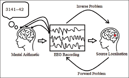
In this article, we focus on understanding the mental workload condition generated by two mental states: mental arithmetic calculation and the mental rest state of a person, using source localisation. Multiple steps are performed to estimate the source activity from the EEG signals. 13 In the literature, various methods have been addressed for the inverse problem, but there is a need to address the correlation between the scalp potentials and source of activity. Hence, in this article we focus on cluster verification to justify that the clusters formed are due to source activity and not any artefacts. Analysis of the mental workload conditions is done by checking the power spectrum and topographic plots for all the signals; then we opt for independent component analysis (ICA), project these components to check the amount of involvement they have in the neural activity and finally cluster all components to get a generalised outcome. Use of fast ICA is seen in the work by Suresha and Parthasarathy, 14 which is used for diagnosis of Alzheimer’s disease. One of the gaps in the literature is to have a model with low computational complexity with the use of EEG signals rather than fMRIs. Also, computational complexity is of utmost importance while applying algorithms to the given dataset. Substantial decrease in time complexity has been observed. A state-of-the-art paper which focuses on brain source localisation can be seen in the work by Bore et al., 15 where authors have used the least absolute penalised solution LAPPS method for sparse source localisation in the presence of Gaussian noise for realistic head models with less computational complexity. Ding and He’s 16 FINE algorithm is used for source localisation in closely spaced sources under low SNR conditions. They have achieved better results compared to the present methods such as MUSIC and RAP-MUSIC. Analysis of EEG signals is done using EEGLAB. 17 The computation time is mentioned in the work by Pirondini et al. 18 for KF-FIS and for SS-KF and SS-FIS. Our algorithm significantly decreases time computations compared to KF-FIS, but little higher as compared to SS-KF and SS-FIS which is seen in Table 1. We also present the results of dipole source localisation in human brain anatomy based on the EEG recording obtained when the person is performing mental arithmetic calculations. Figure 1 shows the basic idea of mental arithmetic state in which the subject performs mental subtraction given the minuend and subtrahend during which the EEG is recorded. The source from the EEG signals is found after removing the artefacts. The solution of the mentioned inverse problem gives the source location of the mental activity.
Comparative Time Computation of Algorithm.
Methods
The dataset was downloaded from physionet.org. 19 There are a total of 36 subjects, and each subject has two files, which have the suffix ‘_1’ for EEG recording before the mental arithmetic calculation and the suffix ‘_2’ for EEG recording while performing the mental arithmetic calculation. All the files are available in an EDF (European data format) for processing.
Source Localisation for Mental Arithmetic State.
The mental arithmetic task includes serial subtraction of two numbers, which includes a four-digit subtrahend and a two-digit minuend. Figure 2 shows the channel allocation with the standard 10/20 system using the 23 channel ‘Neurocom’ EEG system. Electrodes are positioned at parietal, occipital, temporal, central, anterior frontal and frontal lobes of the brain. The EEG signal is sampled at 500 Hz for each channel. We use 19 electrodes for analysis purpose: Fp1, Fp2 in the anterior frontal region; Fz, F3, F4, F7, F8 in the frontal region; Cz, C3, C4 in the central region; Pz, P3, P4 in the parietal region; T3, T4, T5, T6 in the temporal region and O1, O2 in the occipital region. We use MATLAB version R2022b and EEGLAB version 2022.1. The hardware used is 11th Gen Intel(R) Core(TM) i5-1135G7 @ 2.40GHz 2.42 GHz, RAM is 8 GB and system type is a 64-bit operating system, ×64-based processor.
10/20 Channel Locations for 19 Electrodes.
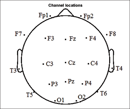
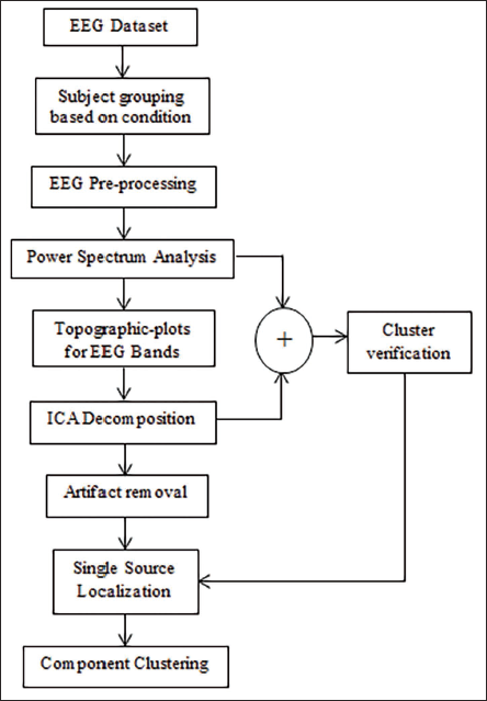
Figure 3 shows the basic flow diagram for ‘CLEVER’, which is used for the analysis of EEG signals for mental arithmetic task. We first analyse the power spectrum for all the signals and find the one having the maximum difference between the two mental states, and then, we plot the topographic plots for the EEG signals at different frequencies such as alpha, beta, gamma, delta and theta. ICA decomposition is done in the second part of the analysis, which helps remove the artefacts from the eyes or the muscle that has been mixed with the EEG signals captured by the electrode. Finally, we do source localisation and cluster these components to understand the mental arithmetic activity generation inside the brain regions.
Proposed Workflow for Analysis of EEG for Mental Arithmetic.
EEG Pre-processing
The EEG signals are pre-processed using a high-pass filter and a low-pass filter with a cutoff frequency of 0.5 and 45 Hz, respectively. A majority of the information is available in these frequency ranges, which are divided in frequency ranges of delta (0.5—4 Hz), theta (4–8 Hz), alpha (8—12 Hz), beta (12—30 Hz) and gamma (30–45 Hz). Power line interference is removed by using a notch filter of 50 Hz frequency.
Power Spectrum Analysis
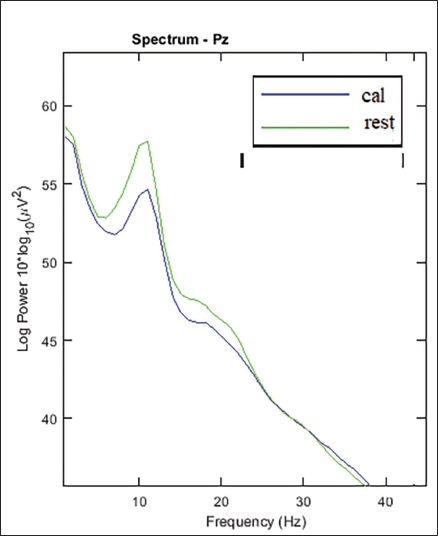
Power spectrum gives the power of different frequency components present in the EEG signals. This analysis is done considering all 36 subjects and for all 19 electrodes. 50% window overlap is considered for calculating the power spectra. Figure 4 shows the power spectrum of the Pz electrode in the parietal area. Considering we have n number of independent files of the EEG data, the average spectral estimate across all the files is given in Equation (1).
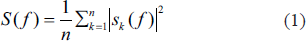
Power Spectrum for the Pz Electrode of the Parietal Lobe.
Topographic Plot for EEG Bands
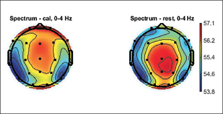
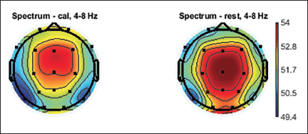
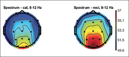
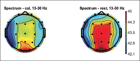
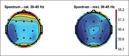
Topographic plots are 2D images of the head looking down from the top. Values from the different electrodes at different frequency bands are interpolated to obtain these graphs. Topographic plots of various frequency ranges are plotted to understand which frequency band shows the signature of the mental workload and rest state. EEG signals are divided into major frequency sub-bands such as delta, theta, alpha, beta and gamma. Figures 5–9 show these plots.
Topographic Plot of Delta Band, 0–4 Hz.
Topographic Plot of Theta band, 4–8 Hz.
Topographic Plot of Alpha Band, 8–12 Hz.
Topographic Plot of Beta Band, 13–30 Hz.
Topographic Plot of Lower Gamma Band, 30–45 Hz.
ICA Decomposition
ICA is done to separate the components which are linearly mixed. The electrodes over the scalp capture not only the electrical activity below its surface but also the activity in the other areas. Hence, this may lead to capture of the artefacts from the eye movement, muscle activity etc. So, ICA helps in removing these artefact components and leaves us with only pure brain-generated signals. This will also help us in source localisation and representing the activity under the brain by means of a dipole. Equation (2) gives ICA source activity.

U = ICA source activity
W = ICA unmixing matrix
X = EEG data (channel × time)
This can be written as

The columns of the inverse weight matrix in Equation (3) give the topographic plots of the independent components. The algorithm used for the decomposition is called INFOMAX. This is one of the algorithms from the blind source separation family which works on information theory. It tries to maximise the entropy of the source and minimise their mutual information. This algorithm tries to make the sources as independent as possible. Consider the joint entropy of the two sources as in Equation (4).
20

The algorithm tries to maximise 
Once we get all the independent components, we manually scan them for artefacts and reject them for further analysis. In all, we have 1,368 components from 72 subjects and 19 electrodes. After artefact rejection, we are left with 1,031 components.
Artefact Removal
The data acquired during the experimentation is corrupted with noise and other artefacts like eye blinks or muscle movements. We manually check for all the components across all the signals and carefully get rid of these artefacts by rejecting them from the study. Thus, clean data is available for further processing.
Source Localisation
Source localisation is an ill-posed inverse problem where we try to find the source given the potential measure on the scalp. Once artefact-free data is available with us, we use these ICA components to fit the dipoles to get similar projections on the scalp maps as with the ICA. We do this as IC maps seem to be dipolar though this does not have a unique solution if more than one source is active. For every scalp map we try to fit a single dipole which fits the best. Equivalent dipole methods are used to fit the best dipole. Equation (6) gives the scalp potentials, and Equation (7) is used for finding the source.

X = scalp recorded potential
L = transfer matrix or head volume conductor model
S = current density vector
n = noise acquired during measurement
The inverse problem is to find S given X:

Realistic BEM head model has been used here for the dipole projections. Though complex, this model represents head in a better way than a simple spherical model with four layers.
Following is the algorithm to find the source of the neural activity:
Component Clustering
To find the source of activity generation in the brain, we do clustering for all the subjects and generalise the results. K means algorithm is used for clustering. We consider 15% residual variance and then recompute the clusters. Residual variance is the measure of the match between the actual data and the standard dipole projections. If the fit is good between the two, the residual variance is very low, and if the fit is bad, it means the residual variance is very high. Equation (8) shows residual variance.

Cluster Verification
We propose the ‘CLEVER’ algorithm, which helps with the verification of the sources and hence verifies the results obtained from the clustering done across the subjects. The electrodes which show maximum power are taken for analysis, that is, the electrodes in the parietal and occipital areas. We then do the ICA decomposition for the subject. We analyse the contribution of the components in each of the electrodes. This contribution is defined as relative percentage variance. More percentage variance shows more contribution of the component in the electrode over the time duration. These results ultimately verify the location of the sources for individual subjects and clusters across the subjects.
Pseudocode
Pseudocode for power analysis is as follows:
For subjects = 1 to n
For electrodes = 1 to m
If electrode(power) > threshold
Return electrode
End if
End for
End for
Pseudocode for components with best fit
For subjects = 1 to n
Remove artefact by filtering
Perform ICA
Calculate residual scalp map variance of best fitting
If residual variance < 15%
Accept component
Else
Reject component
End if
End for
Pseudocode for clustering
Number of dipoles = 1 to n
Initialise number of cluster centre = 1 to k
For all (n−k) dipoles
Find minimum distance
End for
For all k
Calculate distance of dipole from all k
Assign dipole to cluster with min distance
End for
For all k means
Calculate the updated mean value
Continue till no updates in mean
End for
Output k clusters
Results
The analysis based on the mental state of being stressed (calculation state) and the rest state has been recorded in Table 2. It shows the peak power value for every electrode in the alpha band for the mental state of the subject.
Peak Power of Electrodes for Alpha Band.
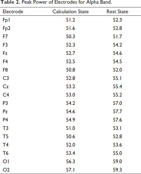
Figure 4 shows the power spectrum of Pz electrodes in the parietal areas of the brain. The maximum power can be seen in the alpha band. It is seen that there is decrease in alpha band during the mental arithmetic calculation state of the subject compared to the rest state. The parietal lobe electrode shows a comparatively greater decrease in alpha value than other lobes of the brain; especially, the Pz electrode shows the maximum difference of 3.1 between the two mental states. It can also be seen that there is occipital lobe involvement.
Average topographic plots of the sub-bands of all 36 subjects are shown in Figures 5–9.
Figure 10 shows the example of ICA for one subject. It is seen that the components get labelled by the features they hold; for example, some components are due to brain activity while some are due to eye and muscle movements. The second component in Figure 10 relates to the eye activity to understand this in detail; we check the component properties.
Independent Component Analysis of One Subject.
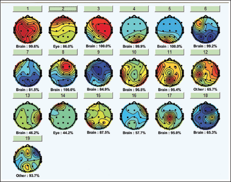
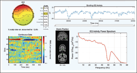
Figure 11 shows the detailed component properties of the second independent component.
Independent Component Number 2 Properties.
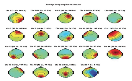
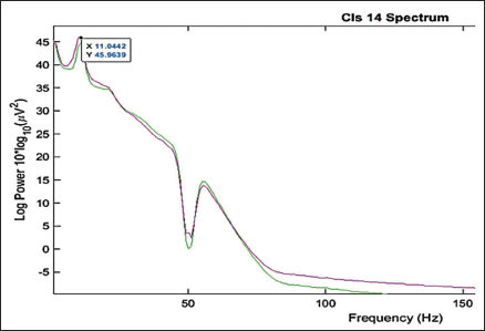
Clustering helps identify similar components across the subject and then locate the global component to view the activity source location. Figure 12 shows the average scalp maps for all the clusters. Cluster 1 is the parent cluster; hence, the scalp maps start from cluster 2 and above. Figure 13 shows the peak power of the alpha band for cluster 14. Figure 14 shows all the clusters with IC components in blue and their centroid in red. Cluster 14 shows the activity near the parietal and occipital areas of the brain. Other clusters which show a high value of the alpha power are clusters 16 and 18; these clusters in Figure 14 also show the activity near the parietal and occipital areas. Next, we plot all the IC components in cluster 14 on a 3D map to understand the exact location of the mental activity; this is shown in Figure 15.
Average Scalp Maps for All the Clusters.
Power Spectrum of Cluster 14.
All Clusters with IC Components.
Cluster 14 in 3D.
Considering 15% residual variance on 1,368 components, we recomputed the clusters given by Artoni et al. 21 This means the number of components which match the single dipole projection with less than 15% of residual variance will be selected for clustering. The total number of independent components after re-computing the residual variance is 518. The total number of the cluster now is 9, considering the first cluster as the parent cluster. Figure 16 shows the average scalp maps of the clusters. Figure 17 shows the power spectrum for cluster 6.
Average Scalp Maps for All the Clusters.
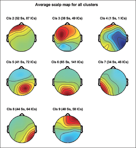
Power Spectrum of Cluster 6.
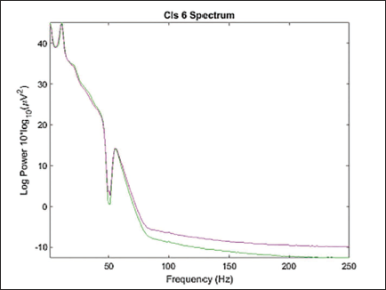
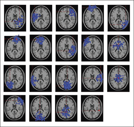
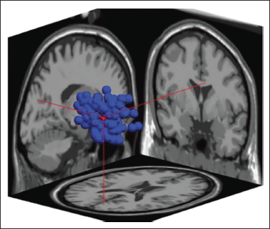
Figure 18 shows the dipoles for all the clusters in blue. Red shows the centroid for the clusters. Figure 19 shows the independent components in 3D for cluster 6. The sagittal view shows the centroid projection on the occipital area.
All Clusters with IC Components.
Cluster 6 in 3D.
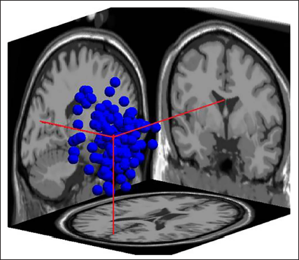
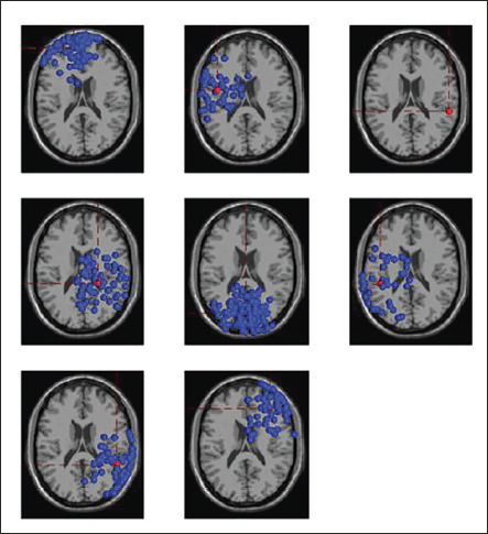
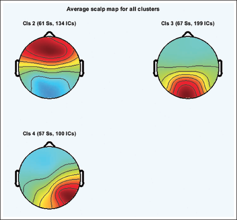
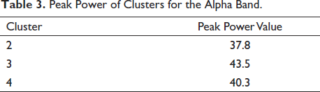
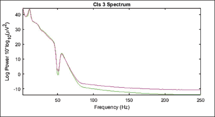
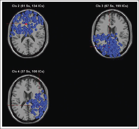
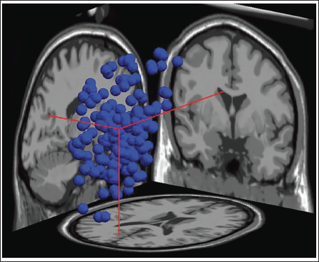
Figure 20 shows the scalp topography of the clusters. Table 3 shows the peak power of all the clusters. Figure 21 shows the spectrum for cluster 3. Figure 22 shows the clusters with the independent components in blue and the centroid in red. Figure 23 shows cluster 3 in the 3D view, and it is seen that the centroid points in the occipital area of the brain.
Average Scalp Maps for All the Clusters.
Peak Power of Clusters for the Alpha Band.
Power Spectrum of Cluster 3.
All Clusters with IC Components.
Cluster 3 in 3D.
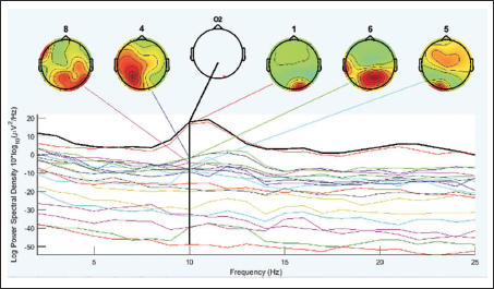
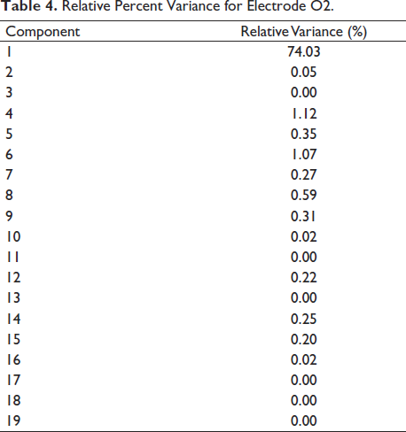
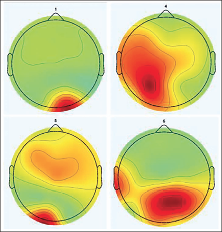
For cluster verification, Figure 24 shows the contribution of components in the electrode. We take a single subject file and analyse the percentage of relative variance for each electrode Table 4 shows the relative variance in percentage. It is seen that component 1 contributes about 74%, which is the highest of all. If we look at component 1 in Figure 24, it clearly shows the activation in the occipital areas of the brain. Figure 25 shows independent component contribution.
Component Contribution for O2 Electrode.
Relative Percent Variance for Electrode O2.
Discussion
It is clearly seen from Figure 7 (which is the topographic plot for the alpha band in the range of 8– 12 Hz) that the parietal and occipital lobes show the involvement during the mental arithmetic calculation. The blinks of the eyes are very clearly seen from the time versus data graph in Figure 11, which shows high and low RMS values of the component while the opening and closing of the eyes. Similarly, we can see the time series graph which shows the blinks. The same is reflected in the dipoles, which show the generation of the activity near the eyes. The power spectrum of the IC also does not show any specific activity near the alpha band, which clearly indicates this IC is not related to the brain signal, but it is an eye blink and should be rejected from the study.
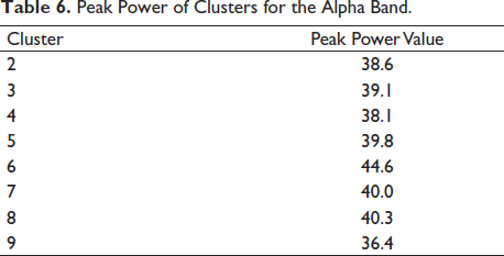
It is seen that cluster 14 holds maximum independent components in Figure 12. We look further to compute the cluster measure and find the maximum power of the clusters. Table 5 shows the cluster number and its respective maximum power for the alpha band. Cluster 14 shows maximum power. It can be clearly seen from Figure 16 that the cluster 6 contains the maximum independent components (141 from) the maximum number of subjects, that is, 65. Cluster 6 in Figure 16 shows the activity in the occipital areas. We find the maximum power of the component spectrum; this maximum power is observed in the alpha band. Table 6 shows the power spectrum of the clusters.
Peak Power of Clusters for the Alpha Band.
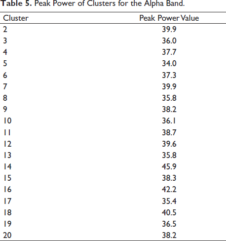
Peak Power of Clusters for the Alpha Band.
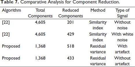
Finally, we remove the artefacts and also compute 15% residual variance on the entire data, which leaves us with 433 components in total from 1,368 components. This is similar to the study by Mannepalli and Routray, where the authors 22 have reduced the solution space to find the most certain sources. In their experimentation test case 1, out of 4,605 sources, the solution space is reduced to 201 certain sources which are active, and with an added 17 dB SNR white noise, the solution space is reduced to 429 most certain sources, which can be seen in Table 7. It is seen that cluster 3 of Figure 20 shows the majority of the components (199), more than 50% pointing in the occipital area.
Comparative Analysis for Component Reduction.
We now analyse all the five electrodes—P3, P4, Pz, O1 and O2—for a single subject. Table 8 gives the component contribution for the electrodes, and in Figure 25, we plot those components individually. It can be clearly seen that the activity of the independent components highlights the fact that the mental arithmetic activity shows high magnitudes in the parietal and occipital areas of the brain. The computational complexity of this algorithm is better than the existing ones as we use the BEM model. To obtain the dipole location, we need to multiply with the inverse transfer matrix and need to calculate only the number of rows, which is nothing but the number of electrodes. This reduces the computational complexity of the algorithms and makes it more efficient. If we consider FEM and FDM methods, direct inversion of the sparse matrix is not possible due to the dimension of the matrix. Large number of unknowns are generated, which cannot be solved directly by computers. In spite of getting good results, there are certain limitation which need to be worked upon. The computational complexity is less but should be further reduced. As the dataset increases, the complexity flares up as well. Second, for more accurate identification of data sources, a large number of electrodes should be considered to improve the resolution of the active sources. The current dataset uses 19 electrodes for the identification of the source activity.
Relative Percent Variance for Electrode O2.
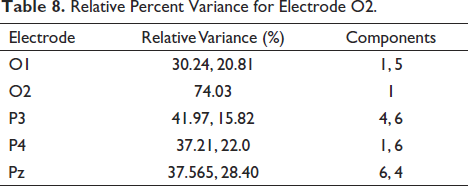
Independent Components 1, 4, 5 and 6.
Conclusion
It is seen that the mental arithmetic activity occurs in areas of parietal and occipital regions of the brain in our analysis. The CLEVER algorithm accurately identifies the components which are responsible for the source of the activity. Here, we see that the clusters formed near the parietal and occipital areas of the brain correlated to the components that have maximum relative variance. The dataset that we use is of mental arithmetic calculations, which is mainly in the parietal area of the brain. This goes along the line of fact where studies have shown that the damage to the parietal area causes problems in solving mathematical problems, difficulty in reading, writing and understanding symbols. Second, occipital areas are associated with visual perceptions. The dataset used here has clearly mentioned that the mathematical problems were orally given to the subject, and they were asked to count without speaking or moving fingers. This points us in the direction that the subjects have used their visual abilities to visualise the numbers and then perform the mathematical calculations. Considering that many people suffer mental stress and this number is growing every single day, our method will provide a cost-effective solution with the use of commercial EEG headset. These headsets have a minimum setup time and are efficient enough for stress diagnoses. With this setup, it will become possible to reach masses in an economical way and quickly. Fast diagnosis will lead to fast treatment. In future, we would like to create a machine learning model which can identify the source of the activity by just using the independent components and also classify these two mental states of workload and rest using machine learning algorithms. This will help in early identification of stress and treatment of mental ailments.
Footnotes
Acknowledgement
Authors gratefully acknowledge the creators of EEGMAT dataset and for making it publicly available.
Authors’ Contribution
All authors contributed to the study’s conception, design and analysis.
Declaration of Conflicting Interests
The authors declared no potential conflicts of interest with respect to the research, authorship and/or publication of this article.
Funding
The authors received no financial support for the research, authorship and/or publication of this article.
ICMJE Statement
This article complies with the International Committee of Medical Journal Editors (ICMJE) uniform requirements for the manuscript.
Statement of Ethics
Not applicable.