Sage Journals: Discover world-class research

Abstract

This article examines the role of domestic and global factors in driving foreign direct investment (FDI) inflows to Asian emerging economies. Conventional panel estimations do not adequately account for the interdependence among countries caused by common global shocks and spatial effects. This article, employing a novel technique, augments the panel cointegration estimations with a proxy for unobserved common factors extracted from the augmented mean group regression. Our estimations control for nonstationarity, endogeneity, cross-sectional dependence, and heterogeneity. Based on the data of six Asian emerging economies from 2000Q1 to 2019Q4, we find a significant impact of both push (global) and pull (domestic) factors in attracting FDI. Our policy implication suggests the sequential opening of the capital account with capital controls and macroprudential regulations in place.

JEL Codes: F21, F30, F41

Keywords

International capital flows FDI cross-sectional dependence emerging markets group-mean FMOLS

1. Introduction

The deregulation of financial markets has led to increased financial integration and volatile international capital flows, posing significant macroeconomic implications for the recipient economy. Emerging and developing economies (EMDEs) saw a surge in net capital inflows after the global financial crisis (GFC) of 2008 due to excess global liquidity, but experienced a significant drop in recent years due to a slowdown in growth and increasing global risk aversion, highlighting the need to study the drivers of these capital flows for designing appropriate policy responses.

Among the different types of capital flows, foreign direct investment (FDI) is a long-term investment and is relatively more stable than short-term investments like foreign portfolio investments (FPI). FDI involves a resident of one economy having control over a company in another economy. Emerging markets have become increasingly important as a destination for FDI from advanced economies (AEs), altering the global landscape of FDI inflows and outflows over the past two decades.

The relevance of studying capital flows to EMDEs also comes from the differing nature of the flows in these economies as compared to those in AEs. It is discussed in the literature that the effect of capital account liberalization increases with the initial level of development in the country but can be counterproductive at low levels of development, thereby making the emerging markets different from the AEs (Edwards, 2001).

The factors affecting capital flows are broadly categorized into pull and push factors. Domestic factors (pull) such as growth differentials from AEs, institutional quality, and financial sector development can attract FDI (Dua & Garg, 2015; Kurul & Yalta, 2017; Wang & Li, 2018). Conversely, global factors (push) include global liquidity abundance and weak growth prospects in mature economies that domestic policy may not be able to influence (Belke & Volz, 2018; Fratzscher, 2012; Nguyen & Lee, 2021). In such cases, domestic policies may affect investment outflows to other countries.

This study provides a deeper insight into the drivers of FDI by taking both domestic and global factors into account. In light of the developments in the global financial markets, there are significant interdependence and spillover effects among the EMDEs, which should be adequately accounted for to avoid misleading inferences. Few papers in the literature on capital flow drivers examine this issue (Belke & Volz, 2018; Kok & Ersoy, 2009; Swamy & Narayanmurthy, 2018), but none of the papers explicitly model cross-sectional dependence (CSD). Therefore, to fill this gap in the existing literature, this study employs robust econometric techniques to explicitly model and control for CSD in examining the determinants of FDI inflows to Asian EMDEs, which are the recipients of the majority of FDI inflows into emerging markets. A focused study on Asian EMDEs is required since these economies are of systemic relevance for the global economy and have significant regional and global implications. The FDI inflows to China, India, Indonesia, Malaysia, the Philippines, and Thailand are examined using the quarterly data from 2000 to 2019.

This study makes several contributions to the literature on capital flows. First, we employ a novel estimation method that controls for CSD, a commonly ignored phenomenon in panel data studies. The results of the study indicate that once the CSD is controlled for in the estimation model, the domestic and global variables are significant in explaining FDI inflows. Second, we use global risk and uncertainty variables to control for the global financial cycle (GFCy) instead of using dummies for specific events. Third, we use quarterly gross FDI flows instead of net flows to capture volatility in inflows and the increasing significance of domestic investors. Fourth, the model examines both domestic and global factors in explaining FDI inflows, based on theoretical and empirical literature. Finally, the study examines the drivers of FDI inflows in Asian EMDEs, contributing to a specific regional analysis for designing capital flow policies.

The article is divided into the following sections: Section 2 discusses the theoretical and empirical literature on the determinants of capital flows and FDI in particular. Section 3 presents the empirical model and the macrotheoretic linkages among the variables, and Section 4 explains the data used along with a detailed discussion of the econometric methodology. Section 5 presents the results of the estimation. Section 6 discusses the results and concludes the article.

2. Literature Review

2.1. Theoretical Considerations

The early phase of theories of FDI referred to the development of investment theories under the classical and neoclassical frameworks. The international differential interest rate theory, capital theory, and portfolio theory (Markovitz, 1959; Tobin, 1958) were the mainstream parts of this phase. The approach postulated that capital flows from countries with a low rate of return to those with a higher rate of return, which eventually leads to an equality of ex-ante real rates of return.

However, the interest rate differential failed to explain the controls that the investors held over institutions in the case of FDI. Hymer (1960) incorporated structural market imperfections into understanding the drivers of FDI. The monopolistic advantages of why a firm invests abroad were the focus of the work of Kindleberger (1969) and Caves (1971). The qualitative methods of determining the flow of FDI were captured in the Product Life Cycle Theory (Vernon, 1992) and the Behavioral Theory by Aharoni (2015). Buckley and Casson (1976) were the first to formalize the various streams of thought into a theory of a multinational enterprise (MNE), namely, the Internationalization Theory of MNE. This is the core theory of FDI, focusing on a firm as a unit of analysis.

The dimension of geography was added to the imperfect market-based theories explaining firm behaviour in the seminal work by Dunning (1980). Ownership, location, and internationalization benefits to MNEs were identified as the major drivers of FDI, and several empirical studies based their analysis on this paradigm, known as the Eclectic Paradigm Approach, proposed by Dunning (1980). This paradigm discusses both the micro and macro determinants of FDI. The factors underlying the ownership and internalization benefits are firm-specific, whereas the location benefits are discussed under macroeconomic considerations.

The theories of international capital flows focus on host country pull factors but also study external push factors. Fernandez-Arias (1996) argues that external factors, such as international interest rates, are a significant determinant of capital flows and presents an analytical model of international portfolio investment based on non-arbitrage and host economy creditworthiness. Structural external factors, such as falling communication costs and the growing importance of institutional investors, played a role in driving private capital flows to emerging economies despite increased world interest rates and the Mexican crisis in 1994.

2.2. Empirical Literature Review

The empirical literature on the drivers of capital flows is extensive and spans across papers analysing gross inflows and net inflows, analysing surges and stops in the flow of capital, examining the drivers of each component of capital inflows separately, and also understanding the capital flow dynamics around and post-GFC. An extensive survey of the literature is available in Hannan (2018) and Koepke (2019).

2.2.1. Pull Factors

With regard to pull factors, higher domestic output and better growth prospects are significant drivers of FDI (Asongu et al., 2018; Belke & Volz, 2018; Dua & Garg, 2015), along with higher domestic productivity (De Vita & Kyaw, 2008). The results regarding better infrastructure attracting capital are mixed (Kumari & Sharma, 2017). Creditworthiness and macroeconomic stability in the host economy are also found to be significant drivers of FDI (Belke & Volz, 2018; Dua & Garg, 2015), with low public debt and high foreign exchange reserves mitigating the negative effects of the global capital flow cycle on many EMDEs.

Exchange rate depreciation (Dua & Garg, 2015) and stability (Belke & Volz, 2018) are found to provide a positive impetus to FDI inflows in the EMDEs, whereas Gastanaga et al. (1998) find that exchange rate distortions in the host country do not exert a detrimental influence on FDI inflows. The role of financial markets measured by stock market capitalization (Mercado & Park, 2011) and stock market development (Wang & Li, 2018) is found to be significant for developing and developed countries, respectively.

Trade openness is found to have a positive and significant effect on FDI inflows in various studies (Asongu et al., 2018; Kumari & Sharma, 2017), while Dua and Garg (2015) and Gastanaga et al. (1998) find evidence of a negative relationship between trade openness and FDI inflows in the economy. Such contrasting results can be attributed to the tariff-jumping motive of FDI inflows, as suggested in the studies.

Kurul and Yalta (2017) and Asongu et al. (2018) find insignificant results for natural resource abundance as a driver for FDI, while Eissa and Elgammal (2020) find positive results for oil exporting countries. The significance of domestic institutions in attracting FDI inflows is found to be robust with control of corruption (Gastanaga et al., 1998; Kurul & Yalta 2017) and governance quality (Wang & Li, 2018), explaining the capital movements in emerging markets. On the contrary, Hannan (2017) does not find a significant impact of institutions on capital flows.

The significant role of financial sector development is discussed by Nguyen and Lee (2021) and Islam et al. (2020), but the former suggests that even in the presence of developed financial markets, domestic uncertainty can discourage FDI flows. Financial openness, often accounted for in the literature in terms of capital controls and macroprudential regulations, forms yet another important driver of FDI inflows. Montiel and Reinhart (1999) find evidence that capital controls imposed by an economy alter the composition of flows (increasing FDI flows and lowering portfolio and short-term flows) and not the magnitude of flows. On the other hand, Forbes and Warnock (2012) find no evidence that capital controls can insulate an economy against capital flow waves.

2.2.2. Push Factors

Empirical research has focused on push factors, such as global liquidity, risk aversion, commodity prices, policy uncertainty, and oil prices, in influencing FDI inflows. Calvo et al. (1993) highlighted the role of push factors in attracting capital to Latin America in the 1990s. Studies by Belke and Volz (2018) and Nguyen and Lee (2021) found that global policy uncertainty has a negative impact on FDI inflows, while Sinha and Ghosh (2021) noted a more pronounced long-term effect on FDI inflows to India. Global credit intermediation is mainly from the financial centres of the world (G4: USA, Euro Area, UK, Japan), and funding conditions are affected globally by the ease of credit in G4 (Cerutti et al., 2014).

Studies have examined the impact of the GFC on international capital flows. Fratzscher (2012) found push factors drove capital flows during the crisis for EMDEs, while pull factors were significant during the recovery. Forbes and Warnock (2021) concluded that post-GFC surge episodes of international capital were less correlated with changes in global risk and driven by different factors. Similarly, Cerutti et al. (2019) used Chicago Board Options Exchange (CBOE) Volatility Index (VIX) and common dynamic factors to measure the GFCy and found that common global shocks do not explain most variation in capital flows.

In line with the theory, studies have found that lower interest rates in AEs are associated with higher capital flows to EMDEs (Dua & Garg, 2015; Montiel & Reinhart, 1999). However, De Vita and Kyaw (2008) find that the effect of foreign interest rates tends to diminish with the longer horizon of the investment, like FDI. The growth differential between the EMDEs and AEs has also emerged as an explanatory variable for FDI flows (De Vita & Kyaw, 2008), but the evidence has been mixed across studies.

3. Empirical Model and Macrotheoretic Linkages

3.1. Model Specification

The empirical model for estimating the drivers of FDI inflows is based on the theoretical and empirical literature and is presented in Equation (1):

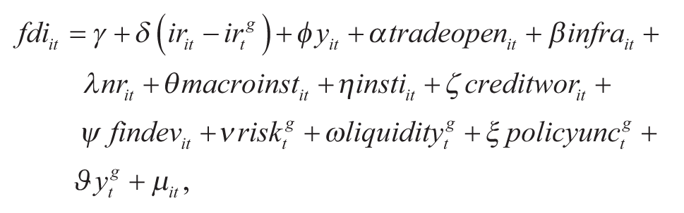
\begin{array}{l} f d i_{i t} = γ + δ (i r_{i t} - i r_{t}^{g}) + ϕ y_{i t} + α t r a d e o p e n_{i t} + β i n f r a_{i t} + \\ λ n r_{i t} + θ m a c r o i n s t_{i t} + η i n s t i_{i t} + ζ c r e d i t w o r_{i t} + \\ ψ f i n d e v_{i t} + ν r i s k_{t}^{g} + ω l i q u i d i t y_{t}^{g} + ξ p o l i c y u n c_{t}^{g} + \\ ϑ y_{t}^{g} + μ_{i t}, \end{array}

(1)

where fdi refers to the FDI inflows, ir is host country’s interest rate, ir^g is global interest rate, y is host country’s market size, tradeopen denotes trade openness, infra denotes infrastructure, nr refers to natural resources, macroinat refers to macroeconomic instability, insti denotes institutional quality, creditwor refers to creditworthiness, findev denotes financial sector development, risk^g is global risk, liquidity^g refers to global liquidity, policyunc^g denotes global uncertainty, and y^g refers to foreign output.

The expected signs are as follows: δ > 0; ϕ > 0; α > or < 0; β > 0; λ > 0; θ < 0; η < 0; ζ > 0; ψ > 0; ν < 0; ω > 0; ξ < 0; and ϑ > or < 0.

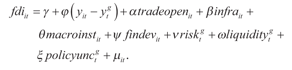
Various interest rate measures were explored for analysis, like the central bank’s policy rate, the 3-month treasury bill rate, the 10-year government securities yield, and the interest rate differential of the mentioned rates with the US economy. But due to missing data and little variation in the policy rate over time, the interest rate was dropped from the final econometric model. Natural resources and institutional quality were also dropped due to the unavailability of quarterly data. To capture the effect of the domestic economy’s growth on FDI inflows, variables related to domestic and US growth rates were combined as a growth rate differential. The relationship between FDI inflows and foreign exchange reserves, which could be capturing the effect of balance of payments identity (Bems et al., 2016) instead of a causal relationship, was dropped from the model.

The final model for econometric estimation is as given in Equation (2).

\begin{array}{l} f d i_{i t} = γ + φ (y_{i t} - y_{t}^{g}) + α t r a d e o p e n_{i t} + β i n f r a_{i t} + \\ θ m a c r o i n s t_{i t} + ψ f i n d e v_{i t} + ν r i s k_{t}^{g} + ω l i q u i d i t y_{t}^{g} + \\ ξ p o l i c y u n c_{t}^{g} + μ_{i t} . \end{array}

(2)

3.2. Macrotheoretic Linkages

This section explains the macrotheoretic linkages between variables in Equation (2). The growth rate differential is used as a measure of expected returns from investments in the host and advanced economies as well as a proxy for market size. A rising growth differential implies increasing growth in the emerging economy or slowing growth in the advanced economy, which could have mixed effects on capital inflows. More money could flow into emerging markets due to better growth prospects or be squeezed due to falling growth in the investor economy.

Trade openness can have mixed effects on FDI as well. Increased trade integration can boost demand for international capital in the domestic economy, while low levels of trade due to tariffs can incentivize investors to enter through FDI. The latter is known as the tariff-jumping nature of FDI. Infrastructure is essential for creating investment opportunities and facilitating FDI inflows.

The macroeconomic instability in an economy elevates its vulnerability to external shocks and makes it more susceptible to crisis. On the other hand, an economy with macroeconomic stability can withstand shocks, thereby making it an attractive destination for domestic and foreign investments. The financial development of an economy spurs FDI inflows as better financial institutions and markets provide better financial services (Nguyen & Lee, 2021).

The notion of “global liquidity” is important for capturing the funding conditions in AEs, as the majority of FDI inflows in emerging markets in the last two decades originated from AEs (Carril-Caccia & Pavlova, 2018). High global liquidity is expected to favourably affect FDI inflows in emerging markets. Global economic policy uncertainty and risk are expected to have a dampening effect on FDI inflows.

4. Data and Methodology

4.1. Data and Variables

The EMDEs have made remarkable progress in the past decades in attracting capital from AEs and strengthening their macroeconomic policies to achieve stable economic growth. Moreover, the share of EMDEs surpassed that of AEs post-2007 in world GDP and has been increasing since then (see Figure 1(a)). Therefore, the present study examines the EMDEs exclusively. Among the global regions, Asia accounts for nearly 39% of the world’s GDP and has been the top contributor to the total global GDP increment in 2021 (World Economic Outlook Report, 2022). Asian economies have shown resilience in the face of global headwinds like the GFC of 2008, high global risk aversion driving capital flight, and the most recent COVID-19 pandemic with moderate growth rates, supportive monetary policy, capital flow controls to counter volatility, and financial stability. In addition, the share of Asian EMDEs is the highest in the total GDP for EMDEs as compared to other counterparts (see Figure 1(b)), reaching 57% in 2021 from 38% in 2000. According to the World Investment Report (2022), developing Asia receives 40% of the world’s foreign investment inflows. Thus, Asian EMDEs provide a suitable sample to study the drivers of foreign investment in emerging markets.

Figure 1.

Source: Authors’ calculations using World Economic Outlook Report (2022).

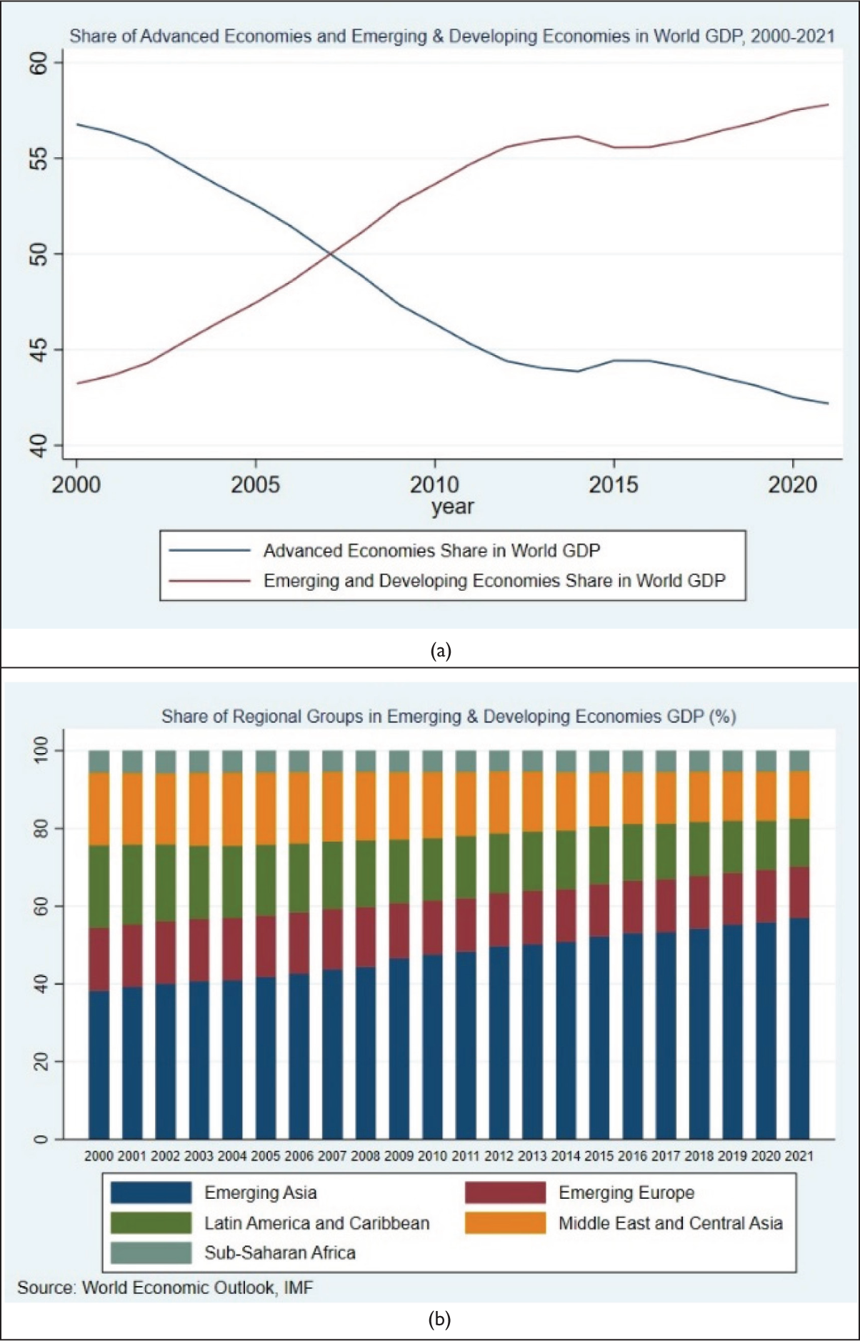
The present study uses data for China, India, Indonesia, Malaysia, the Philippines and Thailand for the period 2000Q1–2019Q4. This set of countries accounts for more than 95% of the GDP of the Asian EMDEs in the period of analysis and is, therefore, representative of the region. Bems et al. (2016) note that though China has the major share of capital flows to the region, the capital flows as a share of its GDP are similar to those of other emerging economies in the region. The period selection is motivated by the data coverage of some of the explanatory variables and also to circumvent the structural break issues in capital flows during the 1980s and 1990s.

Data on FDI inflows in this study are from the IMF BOPS dataset based on the BPM6. The variable used is the “net incurrence of liabilities in direct investment” under the financial account or gross inflows, which includes investment and lending between foreign parents and resident affiliates. This differs from inward FDI investment, which only considers foreign parents’ investment in resident affiliates. FDI inflows are presented as a percentage of GDP to enable comparisons across emerging economies.

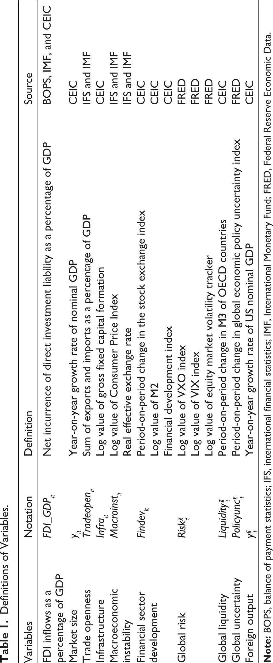
The measures employed in the article for the variables included in Equation (2) are as follows: The growth rate differential variable is measured as a difference between the year-on-year growth rate of the nominal GDP of the host economy and the USA. The GDP growth rate is a proxy for market size and the difference in expected returns due to differing growth prospects.¹ The variable trade openness is measured by the sum of exports and imports as a share of GDP for the emerging economy. Trade openness can have two effects: increased vulnerability to global shocks through contagious financial crises transmitted by trade linkages or increased resilience through trade globalization. The data on gross fixed capital formation (GFCF) are used to measure the infrastructure variable. The macroeconomic instability is captured using the data on the Consumer Price Index (CPI) of the emerging economy, while the real effective exchange rate is used for robustness checks. The variable related to financial sector development is measured using the period-on-period change in the stock market index of the economy. Two additional measures of financial development, the M2 in the economy or the financial development index, are used for robustness checks of the results.

Global variables in the study capture factors like risk, policy uncertainty, and market liquidity that affect capital inflow in emerging economies. Global risk can be measured by indices capturing expected price fluctuations in the market like VIX and CBOE S&P 100 Volatility Index (VXO), which reflect investors’ sentiment and are leading indicators, not indicating immediate market movements. Equity market volatility (EMV) can also be used to measure global risk and moves with VIX. In the estimation, we use the VXO index as a measure of global risk, while VIX and EMV are used for robustness checks. The present study uses the growth of M3 in the OECD countries to measure global liquidity. The variable global uncertainty is measured by the economic policy uncertainty index developed by Baker et al. (2016), which measures policy-related economic uncertainty using newspaper coverage frequency. The definitions of various measures used in estimation are presented in Table 1.

Table 1.

Definitions of Variables.

Variables	Notation	Definition	Source
FDI inflows as a percentage of GDP	FDI_GDP_it	Net incurrence of direct investment liability as a percentage of GDP	BOPS, IMF, and CEIC
Market size	y_it	Year-on-year growth rate of nominal GDP	CEIC
Trade openness	Tradeopen_it	Sum of exports and imports as a percentage of GDP	IFS and IMF
Infrastructure	Infra_it	Log value of gross fixed capital formation	CEIC
Macroeconomic instability	Macroinst_it	Log value of Consumer Price Index	IFS and IMF
Macroeconomic instability	Macroinst_it	Real effective exchange rate	IFS and IMF
Financial sector development	Findev_it	Period-on-period change in the stock exchange index	CEIC
		Log value of M2	CEIC
		Financial development index	CEIC
Global risk	Risk^g_t	Log value of VXO index	FRED
		Log value of VIX index	FRED
		Log value of equity market volatility tracker	FRED
Global liquidity	Liquidity^g_t	Period-on-period change in M3 of OECD countries	CEIC
Global uncertainty	Policyunc^g_t	Period-on-period change in global economic policy uncertainty index	FRED
Foreign output	y^g_t	Year-on-year growth rate of US nominal GDP	CEIC

Note: BOPS, balance of payment statistics; IFS, international financial statistics; IMF, International Monetary Fund; FRED, Federal Reserve Economic Data.

4.2. Econometric Methodology

This section discusses the econometric techniques used in the article to analyse the determinants of FDI for the selected economies. The data collected for the study are aggregate-level macrodata, and static panel methods like fixed effects and random effects are not appropriate in this case as they fail to control for endogeneity and temporal dependencies that may persist in these models. The standard panel fixed-effect model is based on the assumptions of unobserved individual time-invariant effects, slope homogeneity, and independent errors with mean zero and constant variance.² Dynamic panel methods like Holtz-Eakin et al. (1988) and Arellano and Bond (1991) are also not suitable in this context as they require the dynamics to be strictly homogeneous across the different members of the panel. Therefore, the study employs the time series panel techniques of cointegration, which control for endogeneity, cross-sectional heterogeneity, and nonstationarity.

4.2.1. Unit Root Testing

A battery of unit root tests exists for panel data to discern the presence of unit roots in the series. First-generation panel unit root tests, including Im et al.’s (2003) IPS test, Maddala and Wu’s (1999) Fisher-type tests, and Hadri’s (2000) test, are used in the analysis, which do not consider CSD. Second-generation test such as Pesaran (2007) test is also conducted, as it controls for CSD by augmenting the standard Dickey–Fuller and augmented Dickey–Fuller regressions for each cross-section with cross-sectional averages of lagged levels and the first differences of the individual series. The null hypothesis of a unit root is tested against the alternative hypothesis of at least some individual series having unit roots.

4.2.2. Testing for Cointegration

If the linear combination of integrated variables is stationary, then the variables are said to be cointegrated, and it is possible to model the long-run and short-run dynamics simultaneously. There are broadly two types of panel cointegration tests, namely, residual-based methods and error-correction tests. The residual-based methods include Kao (1999), Pedroni (1999, 2004), and Westerlund (2005), which apply a unit root test to the panel regression residuals to determine cointegration. However, one of the disadvantages of residual-based methods is that the long-run parameters for the variables are required to be equal to the short-run parameters for the variables in their differences. This is called common-factor restriction and leads to a significant loss of power (Banerjee et al., 1998). Error-correction model-based tests, such as Westerlund (2007), do not impose this restriction and test for non-cointegration by examining the error correction term in the panel error correction model.

4.2.3. Estimating the Cointegration Vector

For the panels in which the presence of the cointegrating relationship is ascertained using the tests discussed above, the next step is to estimate the cointegrating vector and construct consistent tests of the hypothesis pertaining to the relationship. Though ordinary least squares (OLS) estimates are superconsistent under cointegration, they can contain second-order bias in the presence of endogeneity (Pedroni, 2001), and the associated standard errors are not estimated consistently. The fully modified OLS (FMOLS; Pedroni, 2001) and dynamic ordinary least squares (DOLS; Kao & Chiang, 2001) can correct this problem by producing consistent standard error estimates for testing hypotheses about the cointegrating relationships.

Both methods are single-equation techniques and correct for second-order bias arising due to the endogeneity of regressors by using the dynamics of the regressors as an internal instrument (Pedroni, 2019). FMOLS follows a nonparametric approach to deal with corrections for serial correlation, while DOLS is a parametric technique where leads and lags of differenced regressors are used. Both of these techniques are used in the present study to estimate the cointegrating vector using the group mean approach.

4.2.4. Granger Causality and CSD

The consistent estimation in cointegrated nonstationary panels using FMOLS or DOLS techniques does not establish the direction of causality. The article uses the technique introduced by Dumitrescu and Hurlin (2012), which proposes a simple Granger noncausality test for heterogeneous panel data models. CSD is broadly defined as a contemporaneous correlation among individual members of the panel, left after conditioning on the individual characteristics (Moscone & Tosetti, 2009). Ignoring CSD errors could raise serious concerns about the estimation and result in misleading inferences. The approach used in this article to test for CSD is the one suggested in Pesaran (2007) for panel unit root testing, where the regression equation is augmented with cross-sectional averages.

4.2.5. Estimation with CSD

The article uses a group-mean augmented mean group (AMG) estimator to estimate the panel model, controlling for nonstationarity, cross-sectional heterogeneity, and CSD. This approach is developed in the context of macro production function estimation, where any unobservable common factor represents the total factor productivity (Teal & Eberhardt, 2010).

The procedure is implemented in three steps. The first step is to estimate a pooled regression model by first difference OLS, augmented with year dummies, and the coefficient vector of the (differenced) year dummies is collected, which represents the cross-group average of the evolution of unobserved common factor over time. This is called a common dynamic process (CDP). The process is extracted from the first difference regression, as nonstationary variables and unobservables can bias the estimate in pooled level regression. The pooled regression in the first difference is

Δ y_{i t} = β^{'} Δ x_{i t} + \sum_{t = 2}^{T} γ_{t} Δ D_{t} + e_{i t} ​,

(3)

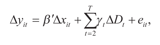
which contains T – 1 year dummies in first differences and from where year dummy coefficients are collected as $\hat{γ_{t}} = \hat{μ_{t}^{*}}$ .

In the second step, the CDP is used to augment the group-specific regression model either by adding it explicitly to the model (as in Equation 4) or by subtracting it from a dependent variable, which implies that it is imposed on each group member with a unit coefficient. The AMG estimator does not treat the unobserved common factors as nuisances and assumes they form CDP, which can be estimated. Eberhardt and Bond (2009) refer to CDP as representing “…the levels-equivalent mean evolvement of unobserved common factors across all countries…”.

y_{i t} = α_{i} + {β^{'}}_{i} x_{i t} + γ_{i} t + λ_{i} \hat{μ_{t}^{*}} + e_{i t} .

(4)

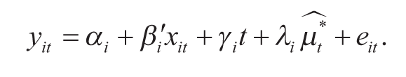
A group-mean average is estimated in the third step by following Pesaran and Smith (1995) as $\hat{β_{A M G}} = N^{- 1} \sum_{i = 1}^{N} \hat{β_{i}} .$

5. Results

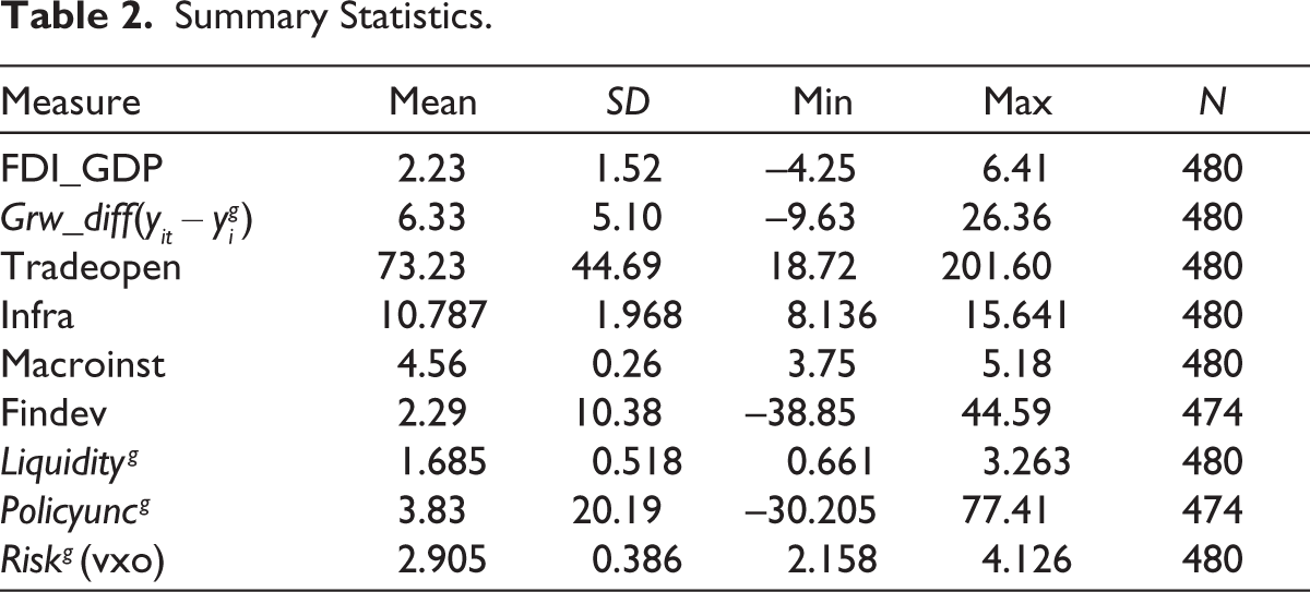
The econometric model in Equation (2) has been estimated in this section using the econometric methodology discussed in the previous section. Table 2 reports the summary statistics of the variables used in the study. The growth rate of the EMDEs has been consistently higher than that of the US throughout the analysis, with a widening differential in the recovery period after the GFC due to faster recovery by EMDEs but narrowing in subsequent years due to falling growth rates in EMDEs.

Table 2.

Summary Statistics.

Measure	Mean	SD	Min	Max	N
FDI_GDP	2.23	1.52	–4.25	6.41	480
Grw_diff(y_{it –} y^g_i)	6.33	5.10	–9.63	26.36	480
Tradeopen	73.23	44.69	18.72	201.60	480
Infra	10.787	1.968	8.136	15.641	480
Macroinst	4.56	0.26	3.75	5.18	480
Findev	2.29	10.38	–38.85	44.59	474
Liquidity^g	1.685	0.518	0.661	3.263	480
Policyunc^g	3.83	20.19	–30.205	77.41	474
Risk^g (vxo)	2.905	0.386	2.158	4.126	480

The panel unit root testing of the domestic (pull) variables found all variables to be integrated in order one. For the global variables, time series unit root testing is done as these variables are cross-sectionally invariant and all the variables are stationary in the first difference. If the majority of the tests for a variable indicate the existence of a unit root, the series is considered to be stationary.³

5.1. Cointegration and Granger Causality Tests

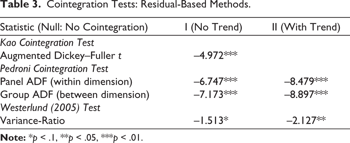
The tests for the presence of cointegration are of two types: residual-based methods and tests based on the error-correction model. Under residual-based methods, the Kao (1999) test, Pedroni (1999, 2004) test, and Westerlund (2005) tests are conducted with and without trend, and the results are presented in the Table 3. The results strongly support the presence of cointegration among the variables. The result based on Westerlund’s (2007) error-correction model also supports the evidence for cointegration.⁴

Table 3.

Cointegration Tests: Residual-Based Methods.

Statistic (Null: No Cointegration)	I (No Trend)	II (With Trend)
Kao Cointegration Test
Augmented Dickey–Fuller t	–4.972***
Pedroni Cointegration Test
Panel ADF (within dimension)	–6.747***	–8.479***
Group ADF (between dimension)	–7.173***	–8.897***
Westerlund (2005) Test
Variance-Ratio	–1.513*	–2.127**

Note: *p < .1, **p < .05, ***p < .01.

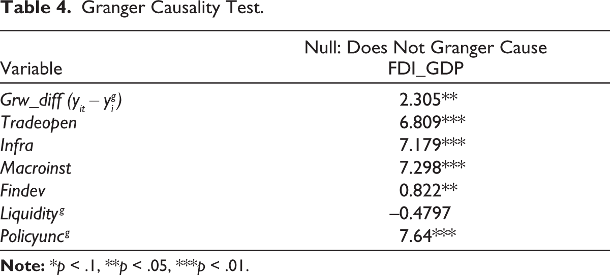
The Granger causality test results are presented in Table 4. Apart from the global liquidity variable, all the other variables Granger-cause the FDI inflows. This result thus justifies the inclusion of these variables in the estimation model as they can improve the predictive performance of the model.

Table 4.

Granger Causality Test.

Variable	Null: Does Not Granger Cause FDI_GDP
Grw_diff (y_{it –} y^g_i)	2.305**
Tradeopen	6.809***
Infra	7.179***
Macroinst	7.298***
Findev	0.822**
Liquidity^g	–0.4797
Policyunc^g	7.64***

Note: *p < .1, **p < .05, ***p < .01.

5.2. Estimation with CSD

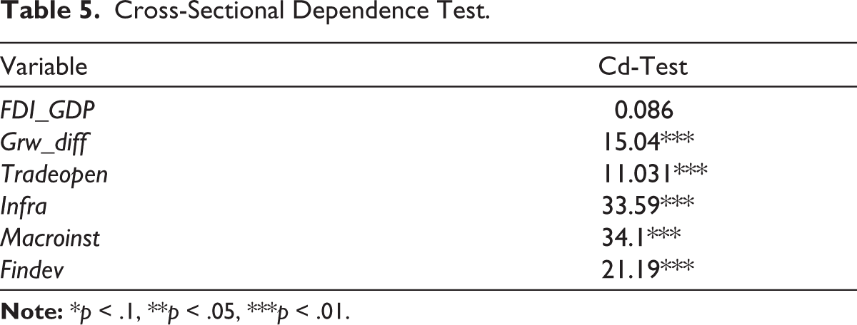
The presence of CSD is checked in the variables to ascertain the technique to be used for estimation, and the results of the same are presented in Table 5. The results for CSD reject the hypothesis of cross-sectional independence except for the FDI inflows variable. This implies that there is a possibility of omitted common effects, spatial effects, and common shocks in the data with spillover effects on the countries.

Table 5.

Cross-Sectional Dependence Test.

Variable	Cd-Test
FDI_GDP	0.086
Grw_diff	15.04***
Tradeopen	11.031***
Infra	33.59***
Macroinst	34.1***
Findev	21.19***

Note: *p < .1, **p < .05, ***p < .01.

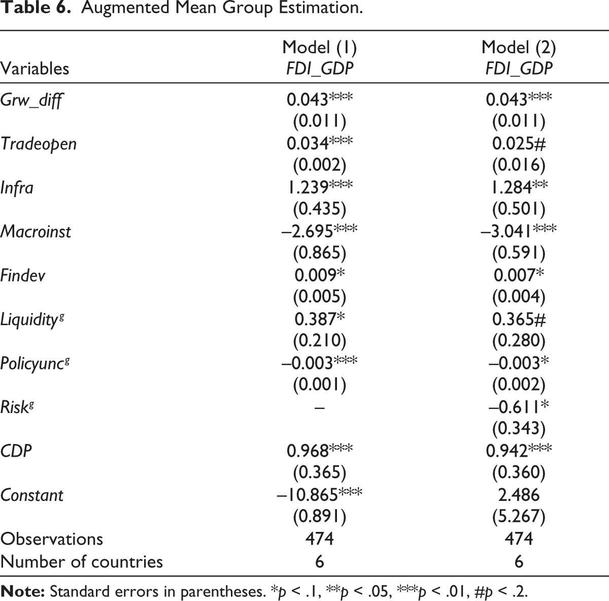
To estimate the model in Equation (2) in the presence of CSD, AMG estimation is done. The AMG estimator deals with nonstationarity, cross-sectional heterogeneity, and CSD.

The regression results are presented in Table 6 for two models. In model (1), the domestic (pull) variables as well as global (push) variables are included, keeping in line with the initial theoretical models of the determinants of FDI, and it is found that growth rate differential, trade openness, infrastructure, macroeconomic instability, and financial development are significant variables in explaining the inflows of FDI and have the expected signs in the estimation. A 1% increase in the growth differential between the emerging economy and the USA increases the FDI inflows by about 0.04% of GDP, while a 1% increase in trade openness increases the FDI inflows by 0.03% of GDP. An increase in macroeconomic instability, measured by the log of CPI, decreases the FDI inflows, while the infrastructure variable has a significant positive impact on FDI inflows. The results of this model provide support for the significance of global variables along with domestic variables. A 1% increase in the growth rate of global liquidity increases FDI inflows by 0.38% of GDP, while economic policy uncertainty is found to have a negative impact.

In addition to the variables in model (1), model (2) includes the global risk variable to control for the GFCy, defined by Cerutti et al. (2019) as “…(high) commonality in financial conditions, manifest in capital flows, driven by observable global determinants…”. The global risk variable negatively affects FDI inflows to Asian EMDEs. Controlling for the GFCy does not alter the significance of push and pull factors. The variable titled CDP in the regression results is the CDP, which is the coefficient vector of year dummies in the first difference regression under the AMG estimation technique. The CDP is explicitly added to the model to control for CSD. However, the AMG estimation results fail to control for endogeneity in the model.

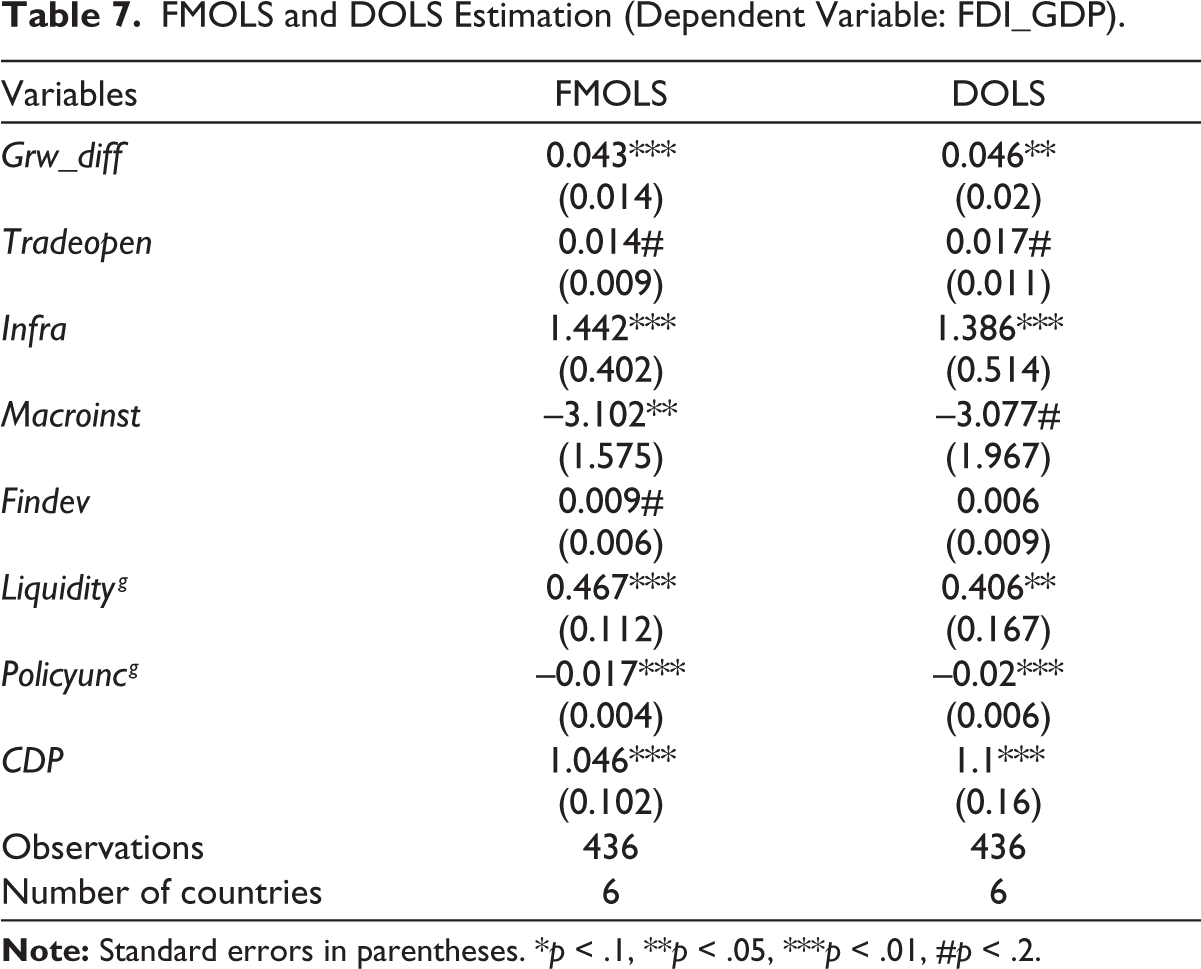
To control for endogeneity along with CSD, we extract the CDP from the AMG estimation of model (1) from Table 6 and use it as an additional regressor of model (1) in FMOLS and DOLS estimations in Table 7.⁵ Using this approach to estimation, we can estimate the long-run cointegrating relationship between FDI and its determinants. The final estimation output controls for CSD in the FMOLS and DOLS estimations, along with endogeneity, cross-sectional heterogeneity, and nonstationarity.

The regression results using FMOLS and DOLS are presented in Table 7. These results improve upon the AMG estimation in Table 6 by controlling for endogeneity among the variables. The growth rate differential between the host economy and the USA, the physical infrastructure, and macroeconomic stability emerge as significant variables in attracting FDI to Asian emerging economies, along with global liquidity. However, global economic policy uncertainty continues to affect FDI inflows negatively. The results are tested under various robustness checks.⁶

Table 6.

Augmented Mean Group Estimation.

Variables	Model (1) FDI_GDP	Model (2) FDI_GDP
Grw_diff	0.043*** (0.011)	0.043*** (0.011)
Tradeopen	0.034*** (0.002)	0.025# (0.016)
Infra	1.239*** (0.435)	1.284** (0.501)
Macroinst	–2.695*** (0.865)	–3.041*** (0.591)
Findev	0.009* (0.005)	0.007* (0.004)
Liquidity^g	0.387* (0.210)	0.365# (0.280)
Policyunc^g	–0.003*** (0.001)	–0.003* (0.002)
Risk^g	–	–0.611* (0.343)
CDP	0.968*** (0.365)	0.942*** (0.360)
Constant	–10.865*** (0.891)	2.486 (5.267)
Observations	474	474
Number of countries	6	6

Note: Standard errors in parentheses. *p < .1, **p < .05, ***p < .01, #p < .2.

Table 7.

FMOLS and DOLS Estimation (Dependent Variable: FDI_GDP).

Variables	FMOLS	DOLS
Grw_diff	0.043*** (0.014)	0.046** (0.02)
Tradeopen	0.014# (0.009)	0.017# (0.011)
Infra	1.442*** (0.402)	1.386*** (0.514)
Macroinst	–3.102** (1.575)	–3.077# (1.967)
Findev	0.009# (0.006)	0.006 (0.009)
Liquidity^g	0.467*** (0.112)	0.406** (0.167)
Policyunc^g	–0.017*** (0.004)	–0.02*** (0.006)
CDP	1.046*** (0.102)	1.1*** (0.16)
Observations	436	436
Number of countries	6	6

Note: Standard errors in parentheses. *p < .1, **p < .05, ***p < .01, #p < .2.

6. Discussion and Conclusion

In this article, we focus on controlling for CSD while studying the determinants of FDI inflows to Asian EMDEs. FDI in these economies is market-seeking and influenced by the growth rate differential between the host and AEs. A higher growth rate of nominal GDP in the emerging economy attracts FDI from AEs, and decreasing growth prospects in the advanced economy may increase the differential, making investment in the emerging economy more attractive.

Trade openness is important in attracting FDI inflows, but we do not find evidence of the tariff-jumping nature of FDI in Asian EMDEs. The physical infrastructure facilitates smooth and successful business operations, thereby attracting FDI. Price stability, indicating the government’s credibility in controlling inflation, is a measure of macroeconomic stability in the study. Low and stable inflation attracts FDI by ensuring efficient allocation of resources and providing better long-term investment opportunities. However, short-term financial conditions have an insignificant effect on FDI, which may be more relevant for attracting short-term capital such as FPI (Belke & Volz, 2018).

The study found that global variables, including global liquidity, economic policy uncertainty, and global risk, are significant in explaining FDI inflows to emerging economies, with global liquidity having a positive effect while economic policy uncertainty has a negative effect. The results are robust to changes in the measurement of variables pertaining to global risk, financial development, and macroeconomic instability. The data analysis of FDI determinants for Asian EMDEs supports the theoretical model (Dunning, 1980) of locational factors and also supports the significance of global factors in attracting FDI.

International capital flows provide much-needed financing capital to emerging markets to enhance their productive capabilities over the course of development. The investment in infrastructure building, manufacturing sector growth, and other long-term projects entails huge investments, both domestically and from abroad. A study on the drivers of FDI inflows is essential for emerging markets to design policies regarding and response mechanisms to capital flows. The results of the study indicate that domestic (pull) factors are equally important as global (push) factors in attracting FDI. The policies focused on enhancing growth prospects in the economy, the state’s investment in physical infrastructure, and ensuring macroeconomic stability make an economy attractive for FDI. An economy needs to focus on enhancing trade integration, lowering tariff and nontariff barriers, and refraining from recurrent changes in trade policy to attract FDI.

We find that external (global) factors are at least as important as pull factors in explaining the movement of FDI to emerging markets, unlike the various studies finding contrary evidence (Belke & Volz, 2018; F¨orster et al., 2014). To insulate the economy from adverse global factors and reduce vulnerability to shocks, capital flow measures like capital controls and macroprudential policies should be put in place by emerging markets. It also entails opening up capital accounts gradually and sequentially to circumvent the negative consequences of financial globalization and have the growth-enhancing effect of FDI.

The limitation of the study is the unavailability of data for some determinants of FDI inflows at a quarterly frequency, like the institutional quality and natural resource abundance. As part of future research on the subject, the role of domestic macroeconomic factors in affecting the sensitivity of capital flows to external factors could be studied. Moreover, the determinants of the common factors causing CSD in emerging markets could be examined. To understand the role of global factors in cross-border FDI movement, the effect on FDI outflows could be examined as well.

Footnotes

Declaration of Conflicting Interests

The authors declared no potential conflicts of interest with respect to the research, authorship, and/or publication of this article.

Funding

The authors received no financial support for the research, authorship, and/or publication of this article.

Notes

References

Aharoni

(2015). The foreign investment decision process. Routledge.

Arellano

, & Bond

(1991). Some tests of specification for panel data: Monte Carlo evidence and an application to employment equations. The Review of Economic Studies, 58(2), 277–297.

Asongu

, Akpan

U. S.

, & Isihak

S. R.

(2018). Determinants of foreign direct investment in fast-growing economies: Evidence from the BRICS and MINT countries. Financial Innovation, 4(1), 1–17.

Baker

S. R.

, Bloom

, & Davis

S. J.

(2016). Measuring economic policy uncertainty. The Quarterly Journal of Economics, 131(4), 1593–1636.

Banerjee

, Dolado

, & Mestre

(1998). Error–correction mechanism tests for cointegration in a single–equation framework. Journal of Time Series Analysis, 19(3), 267–283.

Belke

, & Volz

(2018). Capital flows to emerging market and developing economies. Global liquidity and uncertainty versus country–specific pull factors (Working Paper No. 23/2018). German Development Institute.

Bems

, Catao

, Koczan

, Lian

, Poplawski-Ribeiro

, Jiang

, Liu

, & Yang

(2016). Understanding the slowdown in capital flows to emerging markets. In World economic outlook (pp. 63–99). IMF.

Buckley

P. J.

, & Casson

(Eds), (1976). A long-run theory of the multinational enterprise. In The future of the multinational enterprise (pp. 32–65). Springer.

Calvo

G. A.

, Leiderman

, & Reinhart

C. M.

(1993). Capital inflows and real exchange rate appreciation in Latin America: The role of external factors. Staff Papers, 40(1), 108–151.

10.

Carril-Caccia

, & Pavlova

(2018). Foreign direct investment and its drivers: A global and EU perspective. Economic Bulletin Articles, 4, 60–78.

11.

Caves

R. E.

(1971). International corporations: The industrial economics of foreign investment. Economica, 38(149), 1–27.

12.

Cerutti

, Claessens

, & Rose

A. K.

(2019). How important is the global financial cycle? Evidence from capital flows. IMF Economic Review, 67(1), 24–60.

13.

Cerutti

M. E.

, Claessens

M. S.

, & Ratnovski

M. L.

(2014). Global liquidity and drivers of cross-border bank flows. International Monetary Fund.

14.

De Vita

, & Kyaw

K. S.

(2008). Determinants of capital flows to developing countries: A structural VAR analysis. Journal of Economic Studies, 35(4), 304–322.

15.

Driscoll

J. C.

, & Kraay

A. C.

(1998). Consistent covariance matrix estimation with spatially dependent panel data. Review of Economics and Statistics, 80(4), 549–560.

16.

Dua

, & Garg

(2015). Macroeconomic determinants of foreign direct investment: Evidence from India. The Journal of Developing Areas, 49(1), 133–155.

17.

Dumitrescu

E.-I.

, & Hurlin

(2012). Testing for granger non-causality in heterogeneous panels. Economic Modelling, 29(4), 1450–1460.

18.

Dunning

J. H.

(1980). Toward an eclectic theory of international production: Some empirical tests. Journal of International Business Studies, 11, 9–31.

19.

Eberhardt

, & Bond

(2009). Cross-section dependence in nonstationary panel models: A novel estimator (MPRA Paper 17692). University Library of Munich.

20.

Edwards

(2001). Capital mobility and economic performance: Are emerging economies different? (Working Paper No. 8076). National Bureau of Economic Research.

21.

Eissa

M. A.

, & Elgammal

M. M.

(2020). Foreign direct investment determinants in oil exporting countries: Revisiting the role of natural resources. Journal of Emerging Market Finance, 19(1), 33–65.

22.

Fernandez-Arias

(1996). The new wave of private capital inflows: Push or pull? Journal of Development Economics, 48(2), 389–418.

23.

Forbes

K. J.

, & Warnock

F. E.

(2012). Capital flow waves: Surges, stops, flight, and retrenchment. Journal of International Economics, 88(2), 235–251.

24.

Forbes

K. J.

, & Warnock

F. E.

(2021). Capital flow waves or ripples? Extreme capital flow movements since the crisis. Journal of International Money and Finance, 116, 102394.

25.

F¨orster

, Jorra

, & Tillmann

(2014). The dynamics of international capital flows: Results from a dynamic hierarchical factor model. Journal of International Money and Finance, 48, 101–124.

26.

Fratzscher

(2012). Capital flows, push versus pull factors and the global financial crisis. Journal of International Economics, 88(2), 341–356.

27.

Gastanaga

V. M.

, Nugent

J. B.

, & Pashamova

(1998). Host country reforms and FDI inflows: How much difference do they make? World Development, 26(7), 1299–1314.

28.

Hadri

(2000). Testing for stationarity in heterogeneous panel data. The Econometrics Journal, 3(2), 148–161.

29.

Hannan

S. A.

(2017). The drivers of capital flows in emerging markets post global financial crisis. Journal of International Commerce, Economics and Policy, 8(02), 1750009.

30.

Hannan

S. A.

(2018). Revisiting the determinants of capital flows to emerging markets: A survey of the evolving literature (Working Paper No. 18/214). International Monetary Fund.

31.

Holtz-Eakin

, Newey

, & Rosen

H. S.

(1988). Estimating vector autoregressions with panel data. Econometrica, 56(6), 1371–1395.

32.

Hymer

S. H.

(1960). The international operations of national firms, a study of direct foreign investment (PhD thesis). Massachusetts Institute of Technology.

33.

K. S.

, Pesaran

M. H.

, & Shin

(2003). Testing for unit roots in heterogeneous panels. Journal of Econometrics, 115(1), 53–74.

34.

Islam

M. A.

, Khan

M. A.

, Popp

, Sroka

, & Ol´ah

(2020). Financial development and foreign direct investment the moderating role of quality institutions. Sustainability, 12(9), 3556.

35.

Kao

(1999). Spurious regression and residual-based tests for cointegration in panel data. Journal of Econometrics, 90(1), 1–44.

36.

Kao

, & Chiang

M.-H.

(2001). On the estimation and inference of a cointegrated regression in panel data. In Baltagi

B. H.

(Ed.), Nonstationary panels, panel cointegration, and dynamic panels. Emerald Group Publishing Limited.

37.

Kindleberger

C. P.

(Ed.). (1969). The theory of direct investment. In American business abroad (pp. 2–36). Yale University Press.

38.

Koepke

(2019). What drives capital flows to emerging markets? A survey of the empirical literature. Journal of Economic Surveys, 33(2), 516–540.

39.

Kok

, & Acikgoz Ersoy

(2009). Analyses of FDI determinants in developing countries. International Journal of Social Economics, 36(1/2), 105–123.

40.

Kumari

, & Sharma

A. K.

(2017). Determinants of foreign direct investment in developing countries: A panel data study. International Journal of Emerging Markets, 12(4), 658–682.

41.

Kurul

, & Yalta

A. Y.

(2017). Relationship between institutional factors and FDI flows in developing countries: New evidence from dynamic panel estimation. Economies, 5(2), 17.

42.

Maddala

G. S.

, & Wu

(1999). A comparative study of unit root tests with panel data and a new simple test. Oxford Bulletin of Economics and Statistics, 61(S1), 631–652.

43.

Markovitz

H. M.

(1959). Portfolio selection: Efficient diversification of investments. John Wiley.

44.

Mercado Jr

R. V.

, & Park

C.-Y.

(2011). What drives different types of capital flows and their volatilities in developing Asia? International Economic Journal, 25(4), 655–680.

45.

Montiel

, & Reinhart

C. M.

(1999). Do capital controls and macroeconomic policies influence the volume and composition of capital flows? Evidence from the 1990s. Journal of International Money and Finance, 18(4), 619–635.

46.

Moscone

, & Tosetti

(2009). A review and comparison of tests of cross-section independence in panels. Journal of Economic Surveys, 23(3), 528–561.

47.

Nguyen

C. P.

, & Lee

G. S.

(2021). Uncertainty, financial development, and FDI inflows: Global evidence. Economic Modelling, 99, 105473.

48.

Pedroni

(1999). Critical values for cointegration tests in heterogeneous panels with multiple regressors. Oxford Bulletin of Economics and Statistics, 61(S1), 653–670.

49.

Pedroni

(2001). Fully modified OLS for heterogeneous cointegrated panels. In Nonstationary panels, panel cointegration, and dynamic panels. Emerald Group Publishing Limited.

50.

Pedroni

(2004). Panel cointegration: Asymptotic and finite sample properties of pooled time series tests with an application to the PPP hypothesis. Econometric Theory, 20(3), 597–625.

51.

Pedroni

(2019). Panel cointegration techniques and open challenges. In Tsionas

(Ed.), Panel data econometrics (pp. 251–287). Elsevier.

52.

Pesaran

M. H.

(2007). A simple panel unit root test in the presence of cross-section dependence. Journal of Applied Econometrics, 22(2), 265–312.

53.

Pesaran

M. H.

, & Smith

(1995). Estimating long-run relationships from dynamic heterogeneous panels. Journal of Econometrics, 68(1), 79–113.

54.

Sinha

, & Ghosh

(2021). Impact of economic policy uncertainty on FDI inflows: Evidence from India. In Recent developments in Asian economics international symposia in economic theory and econometrics. Emerald Publishing Limited.

55.

Swamy

, & Narayanamurthy

(2018). What drives the capital flows into BRICS economies? The World Economy, 41(2), 519–549.

56.

Teal

, & Eberhardt

(2010). Productivity analysis in global manufacturing production (Technical report). University of Oxford.

57.

Tobin

(1958). Liquidity preference as behavior towards risk. The Review of Economic Studies, 25(2), 65–86.

58.

Vernon

(1992). International investment and international trade in the product cycle. In Letiche

J. M.

(Ed.), International economic policies and their theoretical foundations (pp. 415–435). Elsevier.

59.

Wang

, & Li

(2018). Determinants of foreign direct and indirect investments from the institutional perspective: A comparative analysis between emerging and mature markets. International Journal of Emerging Markets, 13(5), 1330–1347.

60.

Westerlund

(2005). New simple tests for panel cointegration. Econometric Reviews, 24(3), 297–316.

61.

Westerlund

(2007). Testing for error correction in panel data. Oxford Bulletin of Economics and Statistics, 69(6), 709–748.

62.

World Economic Outlook Report (2022). Countering the cost-of-living crisis, October 22. International Monetary Fund.

63.

United Nations Conference on Trade and Development. (2022). World investment report. UNCTAD.

Drivers of Foreign Direct Investment Inflows to Emerging Asian Economies

Abstract

Keywords

1. Introduction

2. Literature Review

2.1. Theoretical Considerations

2.2. Empirical Literature Review

2.2.1. Pull Factors

2.2.2. Push Factors

3. Empirical Model and Macrotheoretic Linkages

3.1. Model Specification

3.2. Macrotheoretic Linkages

4. Data and Methodology

4.1. Data and Variables

4.2. Econometric Methodology

4.2.1. Unit Root Testing

4.2.2. Testing for Cointegration

4.2.3. Estimating the Cointegration Vector

4.2.4. Granger Causality and CSD

4.2.5. Estimation with CSD

5. Results

5.1. Cointegration and Granger Causality Tests

5.2. Estimation with CSD

6. Discussion and Conclusion

Footnotes

Declaration of Conflicting Interests

Funding

Notes

References