Sage Journals: Discover world-class research

Abstract

This study is an attempt to model the co-integrating relation between economic growth and environmental degradation for two countries namely India and China. Although CO₂ emissions has been the proxy for environmental degradation for most research papers, the study also includes a supplementary proxy environment variable viz forest area as a percentage of land area reflecting the depleting green cover. Thus, the study includes gross domestic product (GDP) per capita as the dependent variable and two regressors as carbon dioxide emissions per capita and forest area as a percentage of land area. The study also includes two additional regressors as trade as a percentage of GDP (proxy for trade openness) and domestic credit to the private sector (proxy for financial development), all converted to natural log terms, and the relation between the variables has been tested using autoregressive distributed lag bounds co-integration approach. The results of the study showed that long-run ‘F’ bounds co-integration test of autoregressive distributed lag was accepted for India but was rejected in case of China. For India, temporal causality was also seen to flow from forest area to per capita GDP with negative cause–effect relation, which was confirmed by Toda and Yamamoto (1995, Journal of Econometrics, 66(1–2), 225–250) causality results. Further with respect to India with a significant co-integration results, vector error correction model was worked out and the results showed that error correction (ECM) coefficient (which was found to be negative and significant) showed that the process of movement towards equilibrium was unexpectedly slow at a rate less than 0.01% per period. The main contribution of the study was to include a new proxy ‘forest area’ for environmental degradation and to empirically prove that with the decrease in forest cover there was a rise in economic growth.

Keywords

ARDL Co-Integration F Bounds Test Vector Error Correction Model Temporal Causality

Introduction

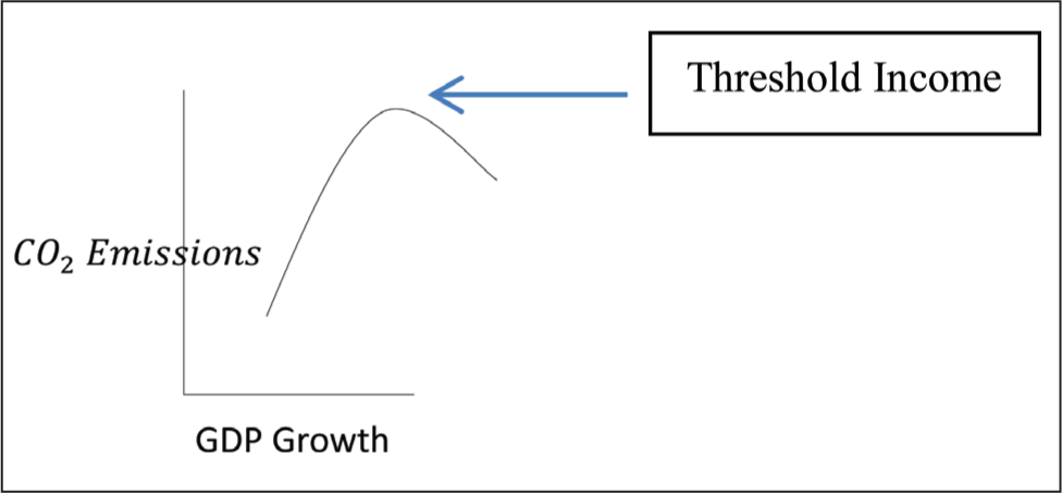
Linking environment with economic growth has today become one of the sought-after research areas in applied economic studies. Earlier studies carried out in 1970s and 1980s had shown how a country with the objective of economic growth tended to compromise on environmental protection. The relation between environment and growth got a big boost when the hypothesis of environmental Kuznets curve or ‘EKC’ was proposed by Grossman and Krueger (1991). These researchers found that economic growth need not be necessarily bad for the environment, as countries do have a tendency towards reduction of environmental degradation once a threshold level of income is reached, beyond which the environmental degradation starts the process of auto reversal. This would mean that the relation between economic growth and environment for a particular country can be either positive or negative, which mainly depends upon its growth path. This relation between environmental degradation and economic growth may switch from positive to negative as a country reaches a level of income/threshold income (Galeotti, 2007).

An ‘inverted U-shaped’ pattern is seen if we plot a time series of economic growth against environmental degradation of a typical developed economy. Such a plot is the ‘EKC’ for that economy (Figure 1).

Figure 1.

Source: The authors.

The EKC hypothesis has, since its development, gained tremendous popularity, so much so that most of the research studies post-development of ‘EKC’ have focused their attention on testing ‘EKC’ on any one or more markets, either using a time series or a panel model. A test of ‘EKC’ model must address two simple questions: first does the inverted U relation hold for the country under-consideration? And second, if the answer to first question is yes, then at what income level we can see the turning point with respect to environmental degradation? The econometric models of co-integration and/or causality are usually applied to detect the relation between the two. Some of the well-researched studies in this area include the study by Sbia et al. (2014), where they carried out research between carbon emissions and economic growth for United Arab Emirates using co-integration and bilateral causality and found strong inter-linkages between the two. Many other studies obtained similar results by applying different co-integration models on diverse markets like Ayobamiji and Kalmaz (2020) on Nigerian markets; Bozkurt and Akan (2014) on Turkey; Chebbi et al. (2011) on Tunisia; Nasir and Rehman (2011) on Pakistan; Hossain and Hasanuzzaman (2012) on Bangladesh; Sikdar and Mukhopadhyay (2018), Kanjilal and Ghosh (2013) on Indian markets; and by Shahani and Bansal (2020) and again by Shahani and Raghuvansi (2020) on India and China. Kanjilal and Ghosh (2013) further confirmed the existence of co-integration and EKC for India only after using a model with regime shift. Now if this is true, then according to Beckerman (1992), the best and surest way to achieve and improve the environment for most countries is to become rich.

On the other hand, there is another class of researchers who do not agree with EKC hypothesis and as a matter of fact tend to hold the opposite view, that is they are of the opinion that economic growth does not impact environmental degradation but it is the other way round, that is environmental degradation leads to economic growth; say deforestation results in more land being made available for agriculture and industries which pushes up the growth rate of the economy. Coondoo and Dinda (2002) concluded that every economy which was on its way to achieve economic growth with minimal impact on environment would be able to achieve its objective only when the economy is ready to sacrifice some part of its economic growth with the quantum of sacrifice being a function of complex relation between energy, environment and income. Again a lot of these research studies actually found this opposite relation that degradation of environment leads to economic growth to hold only after analysing the bidirectional causality between the environmental degradation and economic growth (Bekun et al., 2019; Sari & Soytas, 2009; Sbia et al., 2014; Sebri & Ben-Salha, 2014). Further, shape of the curve, that is the inverted ‘U’ shape relation has been challenged by researchers like Bratt (2012), where after analysing the World Commission on Environment and Development Report 1987 (Our common future) found that a simple ‘U’ shaped curve was more likely as against EKC’s inverse ‘U’ shaped. Similarly, Pal and Mitra (2017) found the relation to be an ‘N’ shaped curve. Finally, we have a third group of researchers who actually found no relation between economic growth and environment (Kohler, 2013; Mhenni, 2005). Here we cannot forget to mention Levinson (2002) who actually demonstrated that one does not require any sophisticated econometric tools but only a simple plot to establish a relation between economic growth and environment.

The review of literature points out that majority of the empirical studies do support the fact that economic growth does impact environment; however, these studies differ significantly when it comes to speed and intensity of exact relation between the variables. This actually impacts the depth of the final outcome of the relation and varies from economy to economy. In terms of variables which have been considered in various empirical studies, growth in income or growth in gross domestic product (GDP) is the proxy variable for economic growth, while for environment degradation, the popular proxy variable has been carbon dioxide (CO₂) or sulphur dioxide emission. Some studies also did consider fine smoke, suspended particulate matter (PM 2.5 or PM 10), nitrogen oxide, nitrogen dioxide, carbon monoxide etc. as their proxies (Akbostancı et al., 2009; Galeotti, 2007). A large number of studies have also included certain control variables in addition to the main variable. Trade openness, urbanization, financial development or financial deepening are some of the commonly used control variables.

Moving in the same direction, this study too has been designed to test the relation between environmental degradation and economic growth, and the sample includes two emerging markets of Asia viz India and China. However, the approach of the study is to test for the opposite viewpoint, that is, impact of environment degradation on economic growth. Some of research studies which also tested for the opposite relation include Bozkurt and Akan (2014), Tiwari (2011a, b) amongst others. The variables which we have included are CO₂ emissions, forest area and GDP per capita. As seen in previous paragraph, CO₂ emissions have been the variable representing environment degradation in most research studies; however, in our study we have also included a second supplementary environment variable viz ‘forest area’, that is, area under the forest cover and thereby makes our study somewhat different from other research studies. The variable ‘forest area’ requires a special mention, as very few studies have included this variable which in our opinion represents a better proxy for environment degradation. The need for inclusion of this variable has arisen as there has been a history of forest area being depleted in the last few decades to make room for agriculture, industry and shelter. The problem is more acute especially in developing economies including China and India. Further to avoid omission bias, the study also includes two more variables as external regressors (control variables), and these include ‘trade as a percentage of GDP’ (proxy for openness) and ‘domestic credit to the private sector’ (proxy for financial development). ‘Trade openness’ enables countries to benefit from transfer of ‘green technologies’ thereby reducing the energy consumption and improving the environment. The ‘domestic credit to private sector’ is a financial development variable and signifies financial resources provided to the private sector by financial institutions which ideally should have a positive impact on the economic growth and level of income.

The study has purposely chosen India and China, as both countries have shown their potential to achieve high economic growth; however, how much of this has been at the cost of environment degradation needs to be researched. For example, in 2018, out of global energy consumption, share of China was 23.6% and 5.8% for India. Further, during the same year these two countries had the highest growth rates of energy consumption; 5.6% (China) and 7.8% (India), this was much higher than average world growth rate of energy consumption which was only 2.9% per annum (Dudley, 2019). Moreover, whereas countries like Japan, France and Germany have managed to reduce absolute fuel consumption over the years, it has been just the opposite for both India and China, where absolute fuel consumption has actually risen during the recent years.

The model used to test the relation under this study is autoregressive distributed lag (ARDL) co-integration approach which was developed by Pesaran and Shin (1999) and modified by Pesaran et al. (2001). The ARDL approach shows, in a single equation, both long-term relation and dynamic interaction between the variables and has gained tremendous popularity amongst the researchers. The technique offers four major advantages over traditional approaches of co-integration: first, it is an ordinary least square based model which is applied after selecting the appropriate lags; second, unit root pre-testing of variables can easily be avoided as both level and first difference stationary variables can easily be incorporated in the model; third, the test can be applied to small samples with a great efficiency and is very useful when we are dealing with annualized data; fourth, by estimating short and long-run relationship simultaneously no long-run information is lost; and finally, the test also includes the benefits of a vector autoregressive (VAR) model, as it can be applied even if some of the regressors are endogenous (Sehrawat & Giri, 2015; Shahani et al., 2018; Srinivasan & Prakasam, 2014,)

The rest of the paper is structured as follows: the next section discusses the research objectives of the study in light of the main objective. The third section describes the data and a brief note on the variables used under the study. The subsequent section gives the methodology used along with hypothesis to be tested. The fifth section provides empirical results of the study and its interpretation. The sixth section gives the conclusion. The final section gives the policy recommendations and scope for further research followed by references and appendices.

Research Objectives

As already stated, the main objective of this paper is to study how the environmental degradation impacts the economic growth of India and China, and keeping this objective in mind, we develop the following research objectives of our study:

To establish single long-run and short-run equations for ARDL specification model between the variables: per capita GDP (as dependent) while CO₂ emissions, forest area, domestic credit to private sector and trade openness as independent variables for two emerging Asian Economies: India and China.

To test the long-term relation using partial ‘F’ bounds test.

To carry out supplementary tests for the ARDL model in terms of (1) serial correlation, (2) stability of the parameters and (3) variable stationarity.

To identify the error correcting mechanism which establishes a binding mechanism for long and short run amongst the co-integrated variables.

To establish the causal relation amongst the variables.

Description of Data and About the Variables

The study considers time series yearly log transformed data for two countries namely India and China, and the period of study is 25 years, that is 1990–2014. The period of study assumes importance as India’s growth rate started picking up post 1990s while China was already enjoying high growth rate during 1990s. Thus, with both the economies on high growth path, it was necessary to assess whether the high growth rates achieved had any relation with environmental degradation in these two economies viz India and China. Another point worth mentioning is that although both the countries had a successful growth rates during this period, the two countries differed in their approaches; whereas growth of China has been mainly driven by their manufacturing sector, India’s growth is mainly a service led growth.

As far as the variables are concerned, a total of five variables have been included in our study, these include per capita GDP at 2010 constant US$ prices, CO₂ emissions metric tonnes per capita, forest area as a percentage of land area, domestic credit to private sector as a percentage of GDP and finally, trade as percentage of GDP. The statistical description of the five variables is given in Table 1. The variables being of different scales have been scaled down to a common format and log transformed before putting them in relation. The data for all the above variables have been taken from website of World Bank (World Development Indicators; www.data.worldbank.org).

Table 1 compares the two countries viz India and China across variables on different parameters viz mean, standard deviation, skewness, kurtosis and normality of distribution for the study period 1990–2014. With respect to some of these variable parameters, India scores above China and these include mean of CO₂ emissions which is less for India than for China. Also, the average area under the forest cover seemed to be in favour of India for the study period. The variables where China scores over India are average GDP per capita, average domestic credit to private sector and trade to GDP.

Table 1.

Statistical Description of Data for Two Countries, India and China on Different Parameters

	CO₂ Emissions		Domestic Credit to Private Sector		Forest Area		GDP Per Capita		Trade to GDP
	India	China	India	China	India	China	India	China	India	China
Mean	1.142	1.797	35.263	108.76	22.742	19.351	973.463	2640.14	34.143	43.43
Standard deviation	0.101	0.495	11.741	16.552	0.659	1.705	328.645	1664.498	13.959	11.73
Skewness	0.152	1.054	0.351	0.0569	–0.358	0.061	0.5377	0.7168	0.2792	0.281
Kurtosis	1.466	2.857	1.413	1.952	2.002	1.737	2.0590	2.2288	1.5040	2.009
Jarque–Bera	2.548	4.655	3.136	1.1569	1.570	1.678	2.1270	2.7601	2.6562	1.352
Probability	0.280	0.098	0.208	0.5608	0.456	0.432	0.3452	0.2515	0.2649	0.509

Source: The authors.

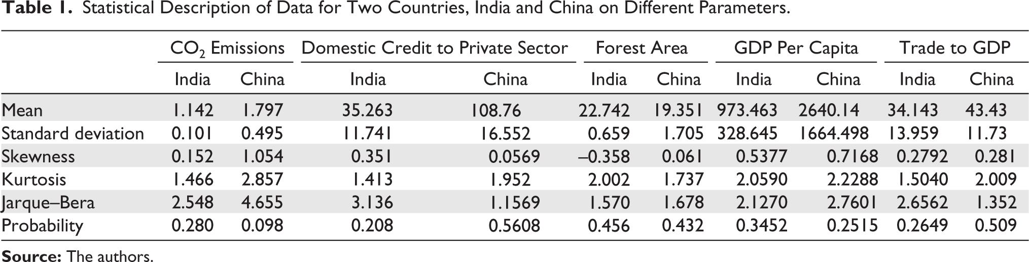
Speaking of variability, the variability in CO₂ emissions during the study period was higher for China than India. India also had lower variability in forest area under cover than China. If we talk of distribution of these variables and try to compare the same with that of a normal distribution, we find that all the distributions are very close to normal (as revealed by Jarque–Bera test statistics with null hypothesis being normal distribution).

Thus, the statistical description of data gives a broader picture of how the variables have behaved over the 25-year period and it is noticed that in terms of CO₂ emissions and forest cover, India seems to have an edge, while growth and trade statistics seemed to be in China’s favour.

Methodology Adopted

ARDL Pre-Requisites

Three pre-requisites for ARDL have been considered in our study and these include (1) variable stationarity, (2) serial correlation test and (3) test for stability of the model and parameters.

Variable Stationarity: ARDL Pre-Requisite I

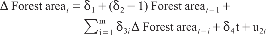
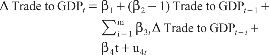
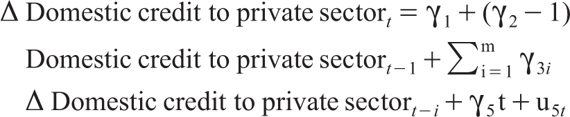
One important pre-requisite for the ARDL model is to check for stationarity of variables, and ARDL model requires that all the variables included in the model to be at stationarity either at level, that is either I(0) or I(1) and no variable should be stationary at I(2) or above. This can easily be known by applying Unit root augmented Dickey–Fuller (ADF) test of stationarity. Hence, we apply ADF test (including intercept and trend) and develop the following five equations for five variables (Equations 1–5).

\begin{matrix} Δ P e r c a p i t a G D P_{t} = θ_{1} + (θ_{2} - 1) P e r c a p i t a G D P_{t - 1} + \\ \sum_{i = 1}^{m} θ_{3 i} Δ P e r C a p i t a G D P_{t - i} + \\ θ_{4} t + u_{1 t} \end{matrix}

(1)

\begin{matrix} Δ F o r e s t a r e a_{t} = δ_{1} + (δ_{2} - 1) F o r e s t a r e a_{t - 1} + \\ \sum_{i = 1}^{m} δ_{3 i} Δ F o r e s t a r e a_{t - i} + δ_{4} t + u_{2 t} \end{matrix}

(2)

\begin{matrix} Δ C O_{2} e m i s s i o n s_{t} = α_{1} + (α_{2} - 1) C O_{2} e m i s s i o n s_{t - 1} + \\ \sum_{i = 1}^{m} α_{3 i} Δ C O_{2} e m i s s i o n s_{t - i} + \\ α_{4} t + u_{3 t} \end{matrix}

(3)

\begin{matrix} Δ T r a d e t o G D P_{t} = β_{1} + (β_{2} - 1) T r a d e t o G D P_{t - 1} + \\ \sum_{i = 1}^{m} β_{3 i} Δ T r a d e t o G D P_{t - i} + \\ β_{4} t + u_{4 t} \end{matrix}

(4)

\begin{matrix} Δ D o m e s t i c c r e d i t t o p r i v a t e \sec ​ t o r_{t} = γ_{1} + (γ_{2} - 1) \\ D o m e s t i c c r e d i t t o p r i v a t e \sec ​ t o r_{t - 1} + \sum_{i = 1}^{m} γ_{3 i} \\ Δ D o m e s t i c c r e d i t t o p r i v a t e \sec ​ t o r_{t - i} + γ_{5} t + u_{5 t} \end{matrix}

(5)

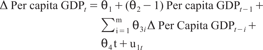
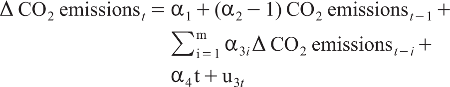
For the Equation (1), where we are testing stationarity for per capita GDP the first term, that is, ‘Δ Per Capita GDPt’ is change in per capita GDP in period t which is regressed against first lag of per capita GDP and lags of change in per capita GDP. The parameter (θ₂ – 1) is the coefficient which decides the stationarity for our variable. The Equation (1) also has two more terms: first term is ‘ $\sum_{i = 1}^{m} θ_{3 i}$ Δ per capita GDP_t-i’ which shows change in per capita GDP in period t-i and is called the augmented variable. Such a term has been added to our stationary Equation (1) to take care of serial correlation. The summation for this term reflects that entire term adds up ‘m’ times (m = number of lags) till the serial correlation is removed from our equation. Another term in our stationary Equation (1) is ‘θ₄t’ which is the trend variable and takes care of deterministic trend so as to focus only on stochastic trend and finally, we have u_1t as the random error term. Similarly, we carry out stationarity tests (Equations 2–5) for other four variables namely forest area, CO₂ emissions, trade to GDP and domestic credit to private sector.

The hypotheses to be tested for stationarity of our variable per capita GDP (Equation 1) have been developed as under:

H₀: θ₂ – 1 = 0 or θ₂ = 1, the per capita GDP is not stationary.

H_a: θ₂ – 1 < 0, per capita GDP is stationary, we apply one sided test to avoid explosive process.

The ADF unit root test of variable stationarity has been reviewed in a number of research studies and most of these studies have arrived at the conclusion that the test suffers from low power. Thus, if we reconsider Equation (1) and focus on the term ‘ $\sum_{i = 1}^{m} θ_{3 i}$ Δ per capita GDP_t-i’, the problem arises with the choice of lags (m). If we select a lower number of lags, clearly autocorrelation would creep in the equation, while if we consider ‘m’ as too large, the power of test will be compromised (Fedorová, 2016).

In order to overcome the limitation of low power of this test, there is a need for a supplementary test of stationarity, and the results of these two must be used together before arriving at the decision whether a variable is stationary or not. Therefore, we carry out a second test of stationarity and the test chosen is the Kwiatkowski–Phillips–Schmidt–Shin (KPSS; 1992) test.

KPSS test develops the time series equation as

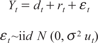
\begin{matrix} Y_{t} = d_{t} + r_{t} + ε_{t} \\ ε_{t} ~ i i d N (0, σ^{2} u_{t}) \end{matrix}

(6)

here ‘d_t’ is the deterministic trend and is given as d_t = $\sum_{i = 1}^{m} β_{i} t^{i}$ , where ‘m’ contains deterministic part of the model, ‘r_t’ is the usual random walk, that is r_t = r_t_-1 + u_t and the variance of random walk is given by $σ_{u}^{2}$ . The KPSS test is unique in the sense that it tests for stationarity with null hypothesis as I(0), while ADF and other tests test for null hypothesis as I(1) (Kwiatkowski et al., 1992)

Null hypothesis H₀: Random walk has ‘0’ variance, that is $σ_{u}^{2}$ =0

Alternative hypothesis H_a: Random walk has positive variance, that is 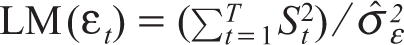$σ_{u}^{2}$ > 0

L M (ε_{t}) = (\sum_{t = 1}^{T} S_{t}^{2}) ​ {\hat{σ}}_{ε}^{2}

(7)

(Note: KPSS follows LM test of hypothesis)

where $S_{t} = \sum_{t = 1}^{T} {\hat{ε}}_{t}$ (t = 1, 2, 3,..T): the residuals are added (at each stage) to get partial sum of residuals (S_t); this is simply cumulative summing or summing up at each stage, for example S₅ would mean sum of first five residuals, S₆ as sum of first six residuals and so on. Now cumulation done at each stage is squared and the value obtained is divided by ${\hat{σ}}_{ε}^{2}$ where ${\hat{σ}}_{ε}^{2}$ is the estimate of the variance for the process ‘ε_t ’of Equation (6).

In simple words, null hypothesis under KPSS is presence of a trend while alternative hypothesis is a possibility of presence of a stochastic root and therefore, we must accept the null hypothesis of KPSS test (If LM(ε_t) has a computed value > critical value, accept the null.) to arrive at the stationarity of a variable.

Serial Correlation: ARDL Pre-Requisite II

Absence of serial correlation or no covariance between residuals and its lag is another pre-requisite of the ARDL model; [cov.( u_t, u_t_-1)] ≠ 0. The presence of serial correlation impacts the efficiency of the parameters and therefore, it must be ensured that the variables are free from serial correlation. To test the serial correlation amongst residuals we apply Breusch-Godfrey Lagrange Multiplier test of residuals and the equation applicable is given as under:

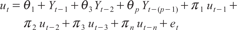
\begin{matrix} u_{t} = θ_{1} + Y_{t - 1} + θ_{3} Y_{t - 2} + θ_{p} Y_{t - (p - 1)} + π_{1} u_{t - 1} + \\ π_{2} u_{t - 2} + π_{3} u_{t - 3} + π_{n} u_{t - n} + e_{t} \end{matrix}

(8)

The variable under consideration: Y_t follows an AR process, ‘u_t’; the error term follows ‘n’ autocorrelation order (number of lags). The applicable test criteria are R² of Equation (8) follows a Chi-square distribution, and the null hypothesis of no serial correlation is accepted when R²(n-p) < χ²n (‘p’ = 1 + the number of lags of the AR equation).

CUSUM Plots: ARDL Pre-Requisite III

Cumulative sum of residuals (CUSUM) are normalized plots of the recursive residuals (which have been cumulated or added at every stage) and are plotted along with upper and lower critical bounds. Here the parameter (or model) is considered stable if the cumulative sum is within the two bounds. The formula for CUSUM is

C_{r} = \sum_{r = 1}^{n - 1} e_{r}

(9)

where e_r are the normalized residuals.

ARDL Model Specification

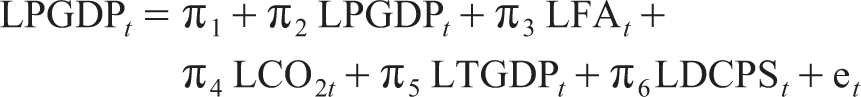
Once our variables satisfy all the model pre-requisites, the next step is to develop our ARDL representation model (originally developed by Pesaran and Shin (1999) and later modified by Pesaran et al. (2001)). In our case we have transformed all the variables into natural log and basic relationship that we would be testing shall be LPGDP = f(LFA, LCO₂, LTGDP, LDCPS) with the beta coefficients reflecting their respective elasticities. The following acronyms have been used: LPGDP is log of per capita GDP, LFA is log of forest area, LCO₂ is log of CO₂ emissions, LTGDP is the log of trade as a percentage of GDP and finally, LDCPS is log of domestic credit to private sector. The ARDL model representation is given as under:

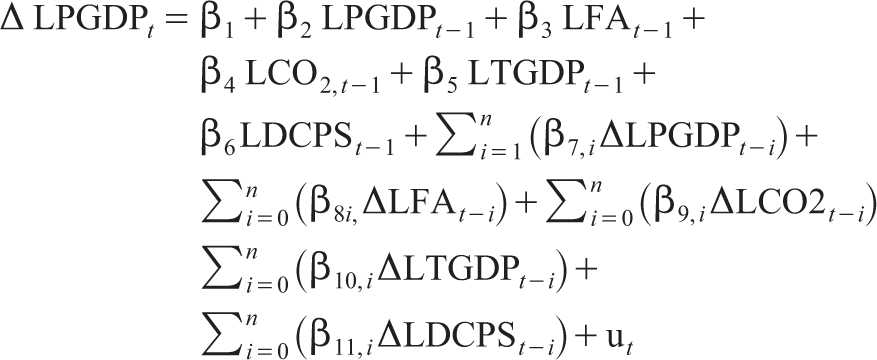
\begin{matrix} \begin{matrix} Δ L P G D P_{t} = β_{1} + β_{2} L P G D P_{t - 1} + β_{3} L F A_{t - 1} + \\ β_{4} L C O_{2, t - 1} + β_{5} L T G D P_{t - 1} + \\ β_{6} L D C P S_{t - 1} + \sum_{i = 1}^{n} (β_{7, i} Δ L P G D P_{t - i}) + \end{matrix} \\ \begin{matrix} \sum_{i = 0}^{n} (β_{8 i,} Δ L F A_{t - i}) + \sum_{i = 0}^{n} (β_{9, i} Δ L C O 2_{t - i}) \\ \sum_{i = 0}^{n} (β_{10, i} Δ L T G D P_{t - i}) + \\ \sum_{i = 0}^{n} (β_{11, i} Δ L D C P S_{t - i}) + u_{t} \end{matrix} \end{matrix}

(10)

where β₁ is the intercept, slope parameters β₂, β₃, β₄, β₅ and β₆ represent the long-run elasticities, while short-run elasticities are represented by β₇, β₈, β₉, β₁₀ and β₁₁ under the ARDL representation. The number of lags ‘n’ are decided by following Akaike information criterion (AIC) Criteria.

Partial ‘F’ Bounds test (Pesaran et al., 2001)

The long-run co-integration test applicable under ARDL representation is partial ‘F’ bounds test. The null hypothesis is no long-term co-integration amongst the variables. Under this test all the long-term coefficients (as elasticities) are jointly made equal to zero and the null hypothesis gets rejected if any of these coefficients is not equal to zero, that is

Null Ho₁: β₂ = β₃ = β₄ = β₅ = β₆ = 0 (from Equation 10 above)

The following shall be accept/reject criteria for our null hypothesis:

Accept the null, if ‘F’_computed < lower bound critical or (3.79)

Reject the null if ‘F’_computed > upper bound critical or (4.85)

No inference if F_computed is between the two bounds or (between 3.79 and 4.85)

Short Run Dynamics and Equilibrium Through ECM

The econometric theory tells us that if the co-integration between two variables is proved then there must be a long-term equilibrium relation between those variables, while in short run we may have a relation which can either be contemporaneous or even a delayed relation (causality). Also, there must be a corrective mechanism to link short-term and long-term behaviour of the two variables, which is called the error correction or the ECM. In our case the short-run variables under ARDL representation are clubbed with the ECM term which is the first lag of residuals obtained through a static model of long-run coefficients. The ECM term shall specify the speed of adjustment to equilibrium and the applicable model is shown as Equation (11).

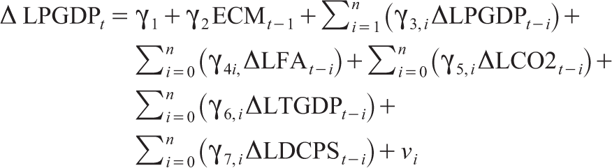
\begin{matrix} Δ L P G D P_{t} = γ_{1} + γ_{2} E C M_{t - 1} + \sum_{i = 1}^{n} (γ_{3, i} Δ L P G D P_{t - i}) + \\ \sum_{i = 0}^{n} (γ_{4 i,} Δ L F A_{t - i}) + \sum_{i = 0}^{n} (γ_{5, i} Δ L C O 2_{t - i}) + \\ \sum_{i = 0}^{n} (γ_{6, i} Δ L T G D P_{t - i}) + \\ \sum_{i = 0}^{n} (γ_{7, i} Δ L D C P S_{t - i}) + v_{i} \end{matrix}

(11)

where γ₃, γ₄, γ₅, γ₆ and γ₇ are the short-run parameters to be estimated and γ₂ is the parameter of lagged ECM term which is obtained by running the contemporaneous variable regression, obtaining the residuals and then taking first lag of residuals, that is Equation (12) given below.

\begin{matrix} L P G D P_{t} = π_{1} + π_{2} L P G D P_{t} + π_{3} L F A_{t} + \\ π_{4} L C O_{2 t} + π_{5} L T G D P_{t} + π_{6} L D C P S_{t} + e_{t} \end{matrix}

(12)

Toda and Yamamoto Causality

We also test for causality of our variables for both the countries, India and China. For China for which the co-integration could not be proved from the results of the study, still we would test for causality as short-run causality can still exist even with no long-run co-integration and the method we use to test causality is Toda and Yamamoto (1995) causality. The Toda–Yamamoto model has restricted and unrestricted models and the test statistic is a modified Wald test which is based upon augmented VAR.

For causality testing; Y₂ → Y₁ , we develop restricted and unrestricted equations as Equations (13) and (14) with AIC determining the optimal length of each variable. We denote ‘h’ and ‘k’ as optimal length of Y₁ and Y₂, respectively.

Restricted Model

Y_{1 i} = λ_{0} + \sum_{j = 1}^{Im a x} α_{j} Y_{2, (t - j)} + \sum_{i = 1}^{h + Im a x} β_{j} Y_{1, (t - j)} + u_{t}

(13)

The above restricted model (Equation 11) has a constant λ₀ and lags of both the variables: Y₁ and Y₂. The model uses ‘h’ which is the optimal length of variable Y₁. The maximum lags of two variables are determined as (1) lags for variable Y₂ = ‘Imax’ that is maximum order of integration of the two variables. (2) Lags for variable Y₁ ‘h+Imax’; ‘h’ is already known, it is the optimal number of lags as per AIC of Y₁. We also have u_t as the error term.

Unrestricted Model

Y_{1 i} = λ_{0} + \sum_{j = 1}^{k + Im a x} α_{j} Y_{2, (t - j)} + \sum_{i = 1}^{h + Im a x} β_{j} Y_{1, (t - i)} + v_{t}

(14)

Unrestricted model (Equation 14) is also based upon augmented lags, that is maximum number of lags of variable Y₁ is given by ‘h+ Imax’ (same as restricted model), while the lags of Y₂ shall be ‘k +Imax’, where ‘k’ is optimal lags for variable Y₂. We also have v_t as the error term.

Null hypothesis: Lagged values of Y₂ do not influence Y₁, that is α_j = 0 (α₁ = α₂ = α₃ …. = 0)

Alternative hypothesis: Lagged values of Y₂ do influence Y₁, that is α_j ≠ 0

Decision criteria: Based upon modified ‘F’ Wald statistics. Reject the null hypothesis if F_{M. Wald} > F_Table at 5%.

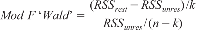
\mod F ‘ W a l d ’ = \frac{(R S S_{r e s t} - R S S_{u n r e s}) / k}{R S S_{u n r e s} / (n - k)}

where RSS is residual sum of the squares, ‘k’ is the degree of freedom of the numerator which is equal to number of parameters to be estimated, ‘n’ being number of observations.

Empirical Results of the Study

Under empirical results of our study, we first discuss the results of stationarity testing of our variables using ADF and KPSS test Statistics for both the countries included in our sample viz India and China. We first apply ADF unit root test and compute tau ‘t’ values and corresponding ‘p’ values for all the five variables both for India and China at level and first difference (Table 2). The results point out that all the variables in case of China are stationary at first difference, while in case of India all the variables except trade to GDP are I(1) stationary with trade to GDP being the only variable which is stationary at I(0) levels. Thus, with a mixture of I(0) and I(1) variables and none of our variables being I(2) or above, ARDL co-integration model was the ideal choice for testing long-run co-integration amongst the variables.

Table 2.

ADF (Unit Root) Test of All the Variables Under Study

Variable	India		China
Variable	‘p’ Value at Level	‘p’ Value at First Difference	‘p’ Value at Level	‘p’ Value at First Difference
Per capita GDP	0.9895	0.0123	0.6230	0.03635
Domestic credit to private sector	0.3225	0.0414	0.4480	0.0080
Forest area	0.2523	0.0409	0.4643	0.04989
Carbon dioxide emissions	0.9873	0.04777	0.3677	0.03723
Trade to GDP	0.0469	0.0033	0.6831	0.01092

Source: The authors.

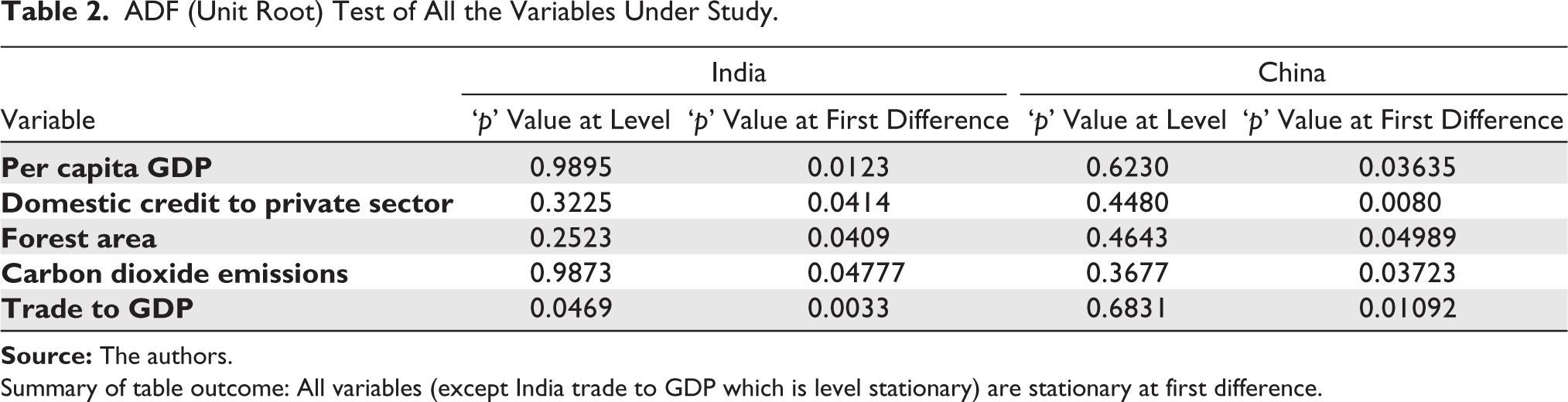
Summary of table outcome: All variables (except India trade to GDP which is level stationary) are stationary at first difference.

Tables 3a and 3b give the results of stationarity testing using KPSS. This test supplements the results of our unit root ADF test. The test results reveal that all the variables are accepting the null of trend stationarity (and absence of unit root) at first difference level. Therefore, considering both these tests ADF and KPSS, we can say with certainty that the requirement of ARDL with respect to stationarity is fulfilled and we can go ahead with development of ARDL co-integration model. However, before we run our ARDL model, we identified the best lag model using AIC criteria. The results showed that both for India as well as China, the AIC was lowest with ‘2’ lags which was identified as the best model and therefore, the ARDL models for both the countries have been built up using lag ‘2’.

Table 3a.

Testing of the Stationary (KPSS) for India

Null Hypothesis	KPSS (Level)	KPSS (1st Diff)	Null: Accept/Reject
Domestic credit to private savings is trend non-random	0.1419	0.1607	Accept both at level and first difference
Per capita GDP is trend non-random	0.1967	0.1017	Accept both at level and first difference
CO₂ levels is trend non-random	0.1767	0.1128	Accept both at level and first difference
Trade as percentage of GDP is trend non-random	0.1101	0.1129	Accept both at level and first difference
Forest area is trend non-random	0.1585	0.1444	Accept both at level and first difference

Source: The authors.

Note: Critical values for KPSS test: 5%, 0.463000 and 1%, 0.739000. KPSS, Kwiatkowski–Phillips–Schmidt–Shin test.

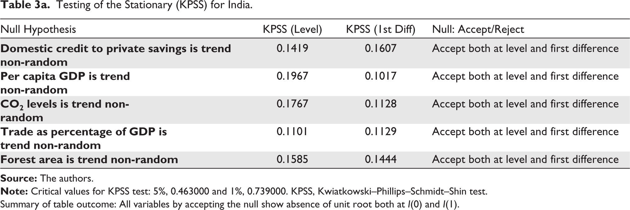
Summary of table outcome: All variables by accepting the null show absence of unit root both at I(0) and I(1).

Table 3b.

Testing of the Stationary (KPSS) for China

Null Hypothesis	KPSS (Level)	KPSS (1st Diff)	Null: Accept/Reject
Domestic credit to private savings is trend non-random	0.0744	0.0894	Accept both at level and first difference
Per capita GDP is trend non-random	0.1949	0.1130	Accept both at level and first difference
CO₂ Levels is trend non-random	0.1786	0.1071	Accept both at level and first difference
Trade as percentage of GDP is trend non-random	0.1155	0.0457	Accept both at level and first difference
Forest area is trend non-random	0.1109	0.1254	Accept both at level and first difference

Source: The authors.

Note: KPSS, Kwiatkowski–Phillips–Schmidt–Shin test.

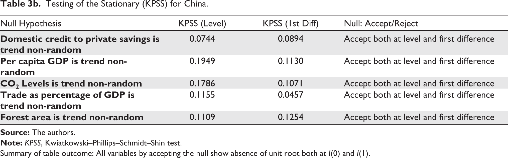
Summary of table outcome: All variables by accepting the null show absence of unit root both at I(0) and I(1).

Table 4 shows the results of our partial ‘F’ bounds co-integration test. The long-run co-integration was accepted for India as shown by the ‘F’ bounds test, where computed value of 8.63 is higher than the table value of 4.85 (upper bound critical) at 5% level of significance; however, the results failed to support any co-integrating relation in case of China as the computed value of 0.747 was lower than the lower bound critical table value of 3.79 at 5% level. Thus, co-integration between variables is established only for India and not for China.

Table 4.

ARDL Co-Integration Partial ‘F’ Test Results (Both the Countries Have Model With Lag 2 as Optimal)

	Relation	‘F’ Bounds Value Computed	Inference
India	LPGDP as a function of LFA, LCO₂, LTGDP and LDCPS	8.63	Null rejected, co-integration established
China	LPGDP as a function of LFA, LCO₂, LTGDP and LDCPS	0.747	Null accepted, co-integration not established

Source: The authors.

Notes: LDCPS, log of domestic credit to private sector; LCO₂, log of CO₂ emissions; LFA, log of forest area; LPGDP, log of per capita gross domestic product; LTGDP, log of trade as a percentage of GDP.

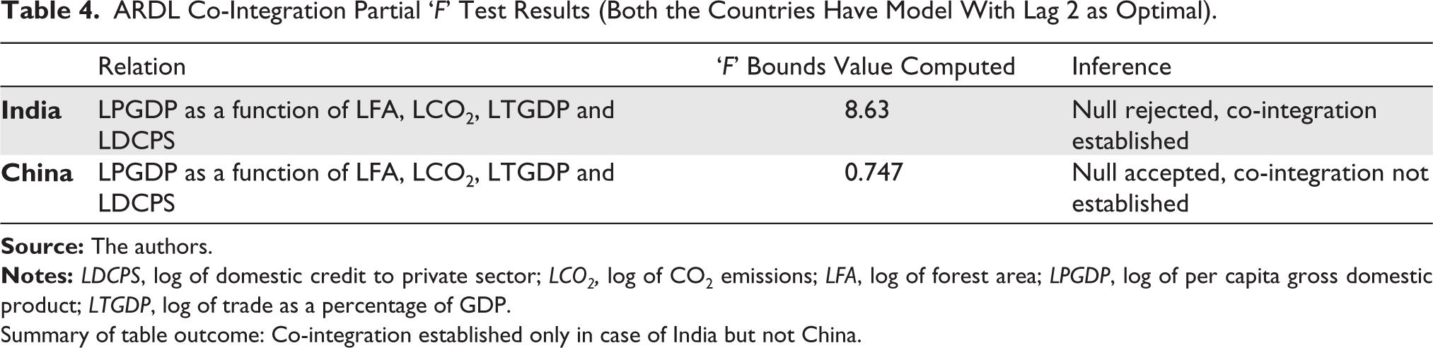
Summary of table outcome: Co-integration established only in case of India but not China.

Table 5 gives the results of our serial correlation test. The results clearly reveal that for both countries, India and China there is absence of serial correlation and the null hypothesis of no serial correlation is accepted in both the countries. The ‘p’ values of observed R² are 0.1939 (India) and 0.17936 (China), which are greater than 0.05 validating the acceptance of null hypothesis.

Table 5.

Results of the Serial Correlation Breusch-Godfrey Lagrange Multiplier Test

	India	China
Observed R-Square	4.24742	3.3181
‘ p ’ Value (Chi Square)	0.1939	0.17936

Source: The authors.

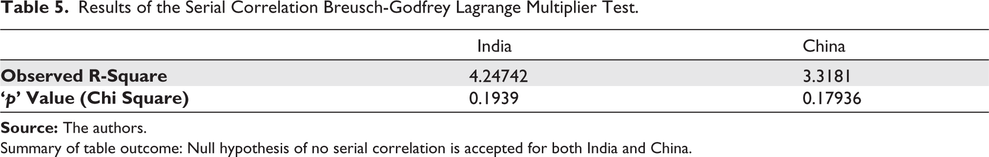
Summary of table outcome: Null hypothesis of no serial correlation is accepted for both India and China.

The next set of results relate to two plots (Figures 2a and b) which give the results of model stability using cumulative sum of residuals (CUSUM). The figures reveal that plots of both India and China are within the ± 5% limits showing stability of these models.

Figure 2(a).

Source: The authors.

Figure 2(b).

Source: The authors.

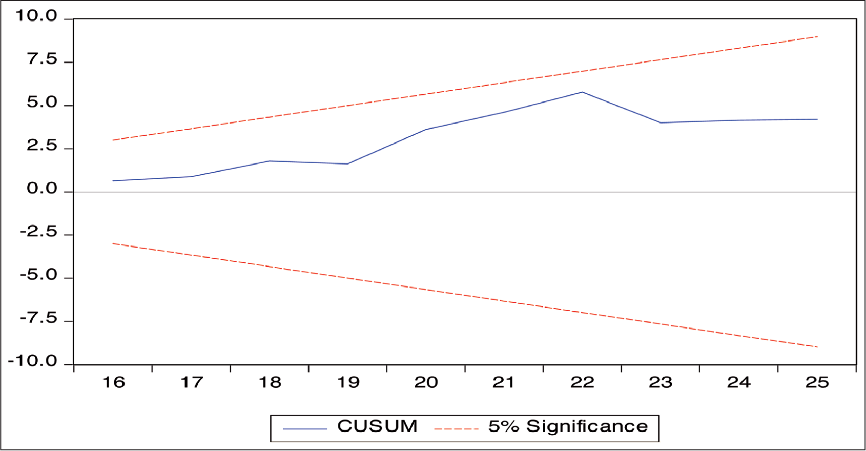
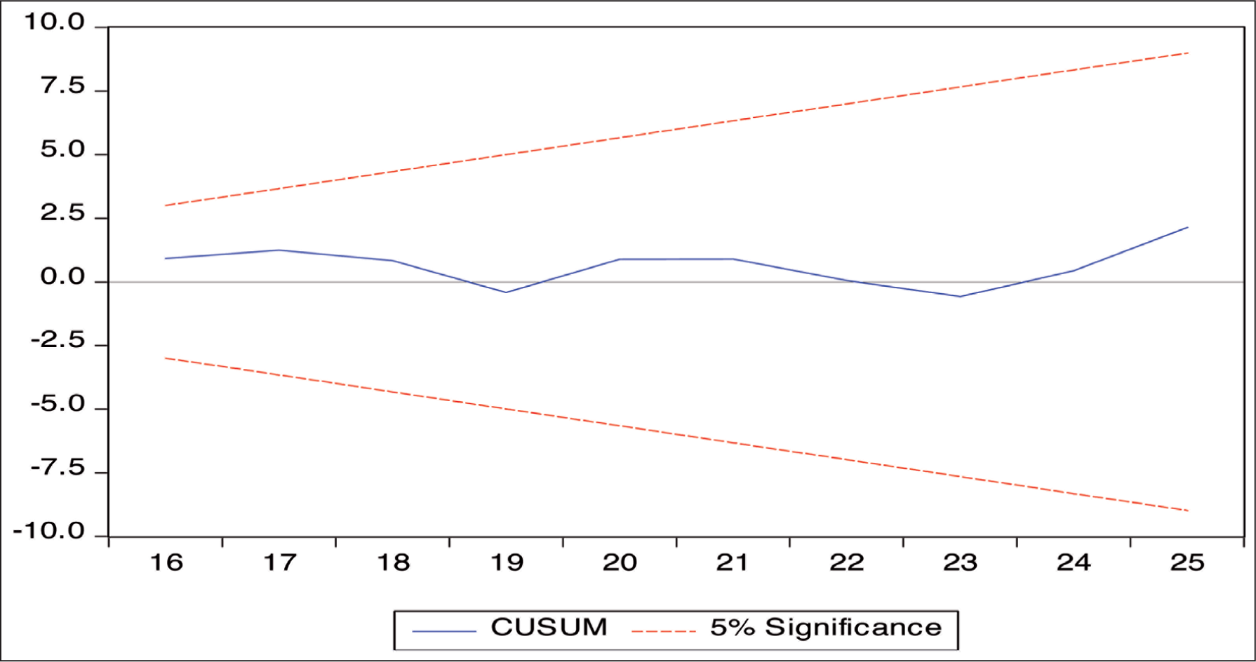
Table 6 gives the results of regression Equation (10) which depicts the short-term relation along with the binding factor between short and long run, that is error correction term viz ECM(−1) and implied temporal causality. It is to be noted that Table 6 includes ECM term only for India but not for China, as long-term co-integration was not proved for China in our study. For India, ECM term is negative and also significant at 5% (corresponding ‘p’ value is 0.00476), thereby reflecting the movement from short-run to long-run equilibrium in case of India. Thus, with co-integration already proved as given by ‘F’ Bound test for India, we conclude that there is going to be equilibrium between short and long run; however, rate of movement towards equilibrium has been found to be rather slow; less than 0.01% per period for India (as given by ECM coefficient which for India was −0.000195).

Table 6 also gives information on long-run causality (through ECM) and again the direction of causality seems to be moving from independent variable forest area to GDP, as the coefficient of lags of the variable forest area are significant and negative, which implies that in case of India variable forest area is impacting GDP in a negative manner thereby showing that with the decrease in forest cover there was a rise in economic growth, while no such long-run cause–effect relation was noticed for China. As far as short-run causality is concerned we carried out a Toda and Yamamoto (1995) causality test, which makes the variables stationary before carrying out causality tests and the results of the same are given in Table 7. The results reveal that in case of India there is short-run causality moving from forest area to GDP of India. These results must be seen together with results obtained in Table 6, and we therefore conclude that in case of forest area there is both short-run and long-run causality moving towards GDP. Further except the pair of forest area–GDP for India, no other causal relation was proved in the study (Table 7).

Table 6.

Regression Results for Short-Run Relation and Long-Run Causality for Our Optimal Model

Variable	India		China
Variable	Coefficient	Probability	Coefficient	Probability
ECM(−1)	−0.000195	0.00476
D(PGDP(−1))	−0.019391	0.9544	0.755440	0.0044
D(PGDP(−2))	−0.093088	0.7906	−0.186418	0.4089
D(FA)	−2.489428	0.0036	2.845832	0.3863
D(FA(−1))	−3.760888	0.0437	−0.745865	0.5991
D(FA(−2))	−8.639622	0.0979	2.418447	0.1047
D(Co2)	−5.397535	0.0058	−1.69065	0.0865
D(Co2(−1))	−0.220548	0.4479	0.034294	0.7396
D(Co2(−2))	0.307728	0.1202	−0.024495	0.8202
D(TRADE)	0.390800	0.2013	0.136827	0.6753
D(TRADE(−1))	0.113671	0.2183	−0.017306	0.6802
D(TRADE(−2))	0.093945	0.4453	0.010822	0.7883
D(D. CREDIT)	0.066355	0.8498	–0.041216	0.9130
D(D. CREDIT(−1))	−0.084001	0.4777	0.002992	0.9585
D(D. CREDIT(−2))	−0.006773	0.9620	−0.035425	0.4930

Source: The authors.

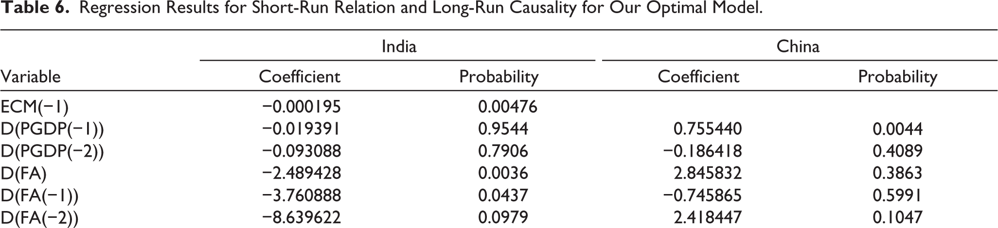
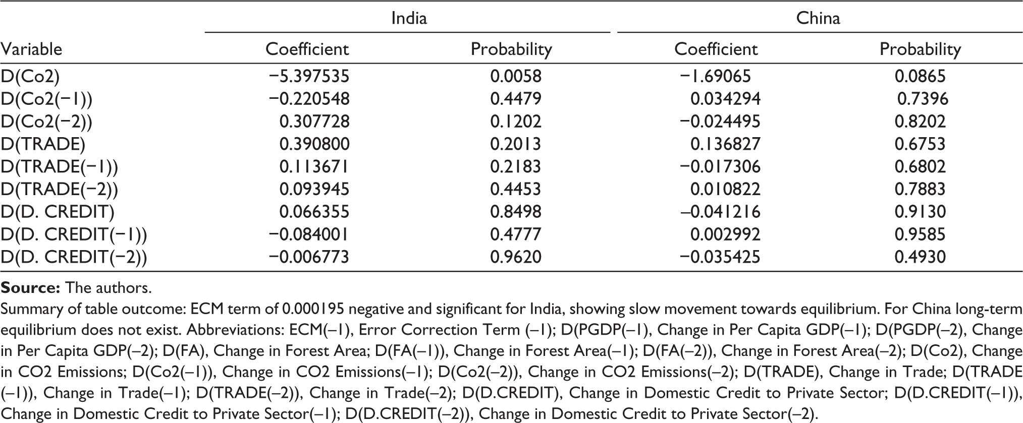
Summary of table outcome: ECM term of 0.000195 negative and significant for India, showing slow movement towards equilibrium. For China long-term equilibrium does not exist. Abbreviations: ECM(–1), Error Correction Term (–1); D(PGDP(–1), Change in Per Capita GDP(–1); D(PGDP(–2), Change in Per Capita GDP(–2); D(FA), Change in Forest Area; D(FA(–1)), Change in Forest Area(–1); D(FA(–2)), Change in Forest Area(–2); D(Co2), Change in CO2 Emissions; D(Co2(–1)), Change in CO2 Emissions(–1); D(Co2(–2)), Change in CO2 Emissions(–2); D(TRADE), Change in Trade; D(TRADE (–1)), Change in Trade(–1); D(TRADE(–2)), Change in Trade(–2); D(D.CREDIT), Change in Domestic Credit to Private Sector; D(D.CREDIT(–1)), Change in Domestic Credit to Private Sector(–1); D(D.CREDIT(–2)), Change in Domestic Credit to Private Sector(–2).

Table 7.

Toda–Yamamoto Causality Test Results (Applied With VAR Augmentation): Dependent Variable (Y1) GDP for India and China

Independent Variable (Y₂)	Obtained Chi Square Value	Probability	Causality
China
Domestic credit to private sector	1.744967	0.4179	No causality
Forest area	4.398084	0.1109	No causality
Carbon dioxide emissions	1.489778	0.4748	No causality
Trade to GDP	5.676291	0.1285	No causality
India
Domestic credit to private sector	7.897114	0.1620	No causality
Forest area	29.40338	0.000	Causality
Carbon dioxide emissions	0.481693	0.7860	No causality
Trade to GDP	0.953360	0.5169	No causality

Source: The authors.

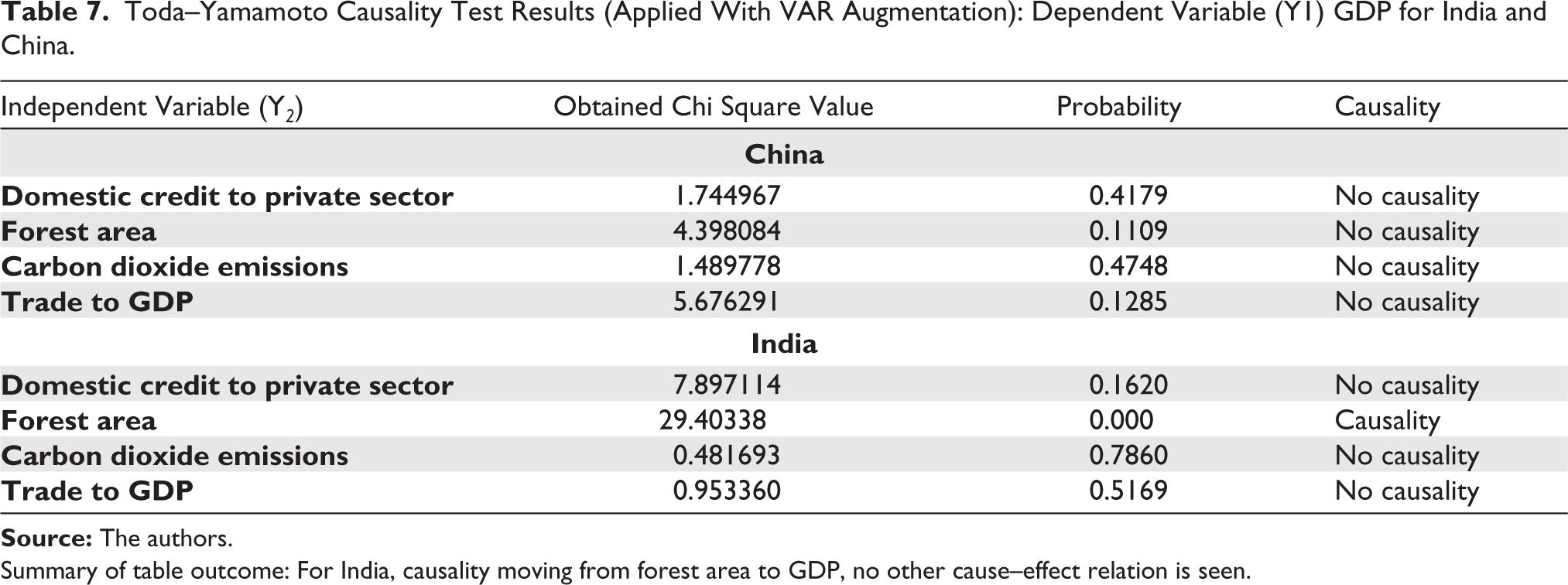
Summary of table outcome: For India, causality moving from forest area to GDP, no other cause–effect relation is seen.

Conclusion

To conclude, the current study was an attempt to empirically model and test the relation between economic growth and environmental degradation for India and China. The study began by discussing the existing prominent studies on the EKC model which could find a positive relation between economic growth and environmental degradation. The paper also discussed some of those studies which held the opposite view, that is environmental degradation impacting the growth process in a country and the same was also extended to this study by taking India and China as two countries. The unique aspect of this study which makes the study different from others was that it considered two proxies for environmental degradation: the CO2 emissions which has been the proxy for environmental degradation for most research papers and a supplementary proxy ‘area under the forest cover’. The econometric tool adopted in the study to check for the relation between environment and economic growth was ARDL bounds co-integration approach, and the model was chosen as it worked at both level and first difference variables. The results of the co-integration was established using partial bounds ‘F’ test. The results of short-run dynamics were clubbed with error correction representation and were shown separately under ARDL model. Before applying the ARDL model, the study also tested for the pre-requisites for this model, that is, tests were conducted for stationarity of variables, serial correlation and model stability.

The results of the study did reveal that long-run co-integration between economic growth and environmental degradation existed for India but was rejected in case of China. These results are consistent with results obtained in Shahani and Bansal (2020) and Shahani and Raghuvansi (2020) on same two countries viz India and China and again by Kanjilal and Ghosh (2013) on India. The non-existence of co-integration between growth and environment for China could be due to their strict policy on energy consumption which is the backbone of clean environment. China has managed to focus on growth while reducing the rate of growth of energy consumption to 5.6% (2018 figures) which is much lower than India’s growth rate of energy consumption 7.8% (2018 figures), although both countries are still much above than average world growth rate of energy consumption of 2.9% (Dudley, 2019). On the other hand, the existence of long-term co-integration in case of India resulted in further investigation into checking for short-run dynamics and temporal causality. For India, temporal causality was also seen to flow from forest area to per capita GDP with negative cause–effect relation, showing decrease in forest cover was associated with rise in economic growth. The lagged ECM coefficient between short and long run or the ECM was negative but significant for India showing that the process of movement towards equilibrium was stable; however, the process of movement was rather unexpectedly slow as the ECM(−1) had a slope coefficient of −-0.000195 which meant that the movement was at a rate less than 0.01% per period.

Policy Implications and Scope for Further Research

There can be few policy implications of the study, first since it is now clear that India’s environmental degradation (proxied by fall in forest cover) does impact country’s economic growth; with variable ‘forest area’ being negatively related to growth, there is a need to ponder about how to balance the two conflicting interests. Clearly, sustainable development is the answer to this problem, wherein the country tries to achieve development without compromising on environment, for example, investing in new technologies which are environment friendly, environmental impact assessment of all new projects, giving reasonable deadlines to existing projects to switch to cleaner technology and so on. Every effort must be made by the government to make all new technologies competitive by giving subsidies, tax holidays or allowing then incentive in the form of tradable carbon credits; the objective being to set an example for traditional technologies and show them the route to shift to environment friendly clean technology.

Further, although both India and China have had high rates of growth for energy consumption, the two economies cannot be compared on the same scale. This is so because whereas India has excelled in the services sector leaving behind the industrial sector, China has mainly thrived on the manufacturing sector. Now with energy requirement being much higher in the manufacturing sector than the services sector, China with a larger manufacturing base, China’s growth rate of energy consumption of 5.6% per annum does not appear to be too high while India’s growth rate of energy consumption of 7.8% per annum appears to be alarming. This also reveals that China’s effort in steadily shifting towards environmentally friendly manufacturing is paying off. As far India goes, the country requires a more serious attempt with respect to sustainable development and shifting to environment friendly technologies, and solution to India’s problem must be searched in those countries which have successfully managed in achieving sustainable development while working under similar circumstances.

The findings of the study also provides useful insight about the further research which could be taken up by the researchers. Researchers could explore why the main environmental variable, that is, CO₂ emissions were not found to be impacting the GDP growth rate of two countries, while the positive co-integration between these variables was found for India under the study. Does this mean that the variables Co₂ and GDP growth of India are co-integrated with no cause–effect relation or it means that the causality exists the other way round, that is, GDP impacting CO₂ which has also been proved in a number of studies. Another explanation for the same could be that there is only contemporaneous between the two variables.

On the other hand, results of the study showed that causality exists between the supplementary environmental variable ‘forest area cover’ and GDP growth of India. Now does this mean that ‘forest area cover” is a better indicator of environment degradation as a variable than Co₂ emissions. If this is true, then why so many research studies which have taken Co₂ emissions as the main proxy variable for environment degradation and have also found a significant relation with the country’s GDP. Does this amount to any omission which these studies have failed to detect? If this is so, that is there is an omission, it is quite likely that CO₂ emissions as the variable would mimic the role of omitted variable thus giving a favorable outcome as shown by most researchers. This needs to be explored by the researchers. There is a strong argument why researchers need to consider different proxies of environment degradation: ‘environment degradation’ is a complex phenomenon and cannot be measured easily and directly like growth or industrial production and therefore, there shall always be a diverse opinion regarding the right proxy for the same. The supplementary proxy taken by the present study ‘forest area cover’ has been arrived at after a lot of research and has indeed proved to be more closely associated with growth and this has been the most important contribution of this study.

Footnotes

Declaration of Conflicting Interests

The authors declared no potential conflicts of interest with respect to the research, authorship and/or publication of this article.

Funding

The authors received no financial support for the research, authorship and/or publication of this article.

References

Akbostancı

, Türüt-Aşık

, & Tunç

G. İ.

(2009). The relationship between income and environment in Turkey: Is there an environmental Kuznets curve? Energy Policy, 37(3), 861–867.

Ayobamiji

A. A.

, & Kalmaz

D. B.

(2020). Reinvestigating the determinants of environmental degradation in Nigeria. International Journal of Economic Policy in Emerging Economies, 13(1), 52–71.

Beckerman

(1992). Economic growth and the environment: Whose growth? Whose environment? World Development, 20(4), 481–496.

Bekun

F. V.

, Alola

A. A.

, & Sarkodie

S. A.

(2019). Toward a sustainable environment: Nexus between CO2 emissions, resource rent, renewable and nonrenewable energy in 16-EU countries. Science of the Total Environment, 657, 1023–1029.

Bozkurt

, & Akan

(2014). Economic growth, CO2 emissions and energy consumption: The Turkish case. International Journal of Energy Economics and Policy, 4(3), 484.

Bratt

(2012). Three totally different environmental/GDP curves. In Sustainable development-education, business and management-architecture and building construction-agriculture and food security. IntechOpen.

Chebbi

H. E.

, Olarreaga

, & Zitouna

(2011). Trade openness and CO 2 emissions in Tunisia. Middle East Development Journal, 3(01), 29–53.

Coondoo

, & Dinda

(2002). Causality between income and emission: A country group-specific econometric analysis. Ecological Economics, 40(3), 351–367.

Dudley

(2019). BP statistical review of world energy. London, UK. 8–9. https://www.bp.com/content/dam/bp/business-sites/en/global/corporate/pdfs/energy-economics/statistical-review/bp-stats-review-2019-full-report.pdf

10.

Fedorová

(2016). Selection of unit root test on the basis of length of the time series and value of AR(1) parameter. Statistika: Statistics and Economy Journal, 96(3), 3.

11.

Galeotti

(2007). Economic growth and the quality of the environment: Taking stock. Environment, Development and Sustainability, 9(4),427–454.

12.

Grossman

G. M.

, Krueger

A. B.

(1991). Environmental impacts of a North American free trade agreement [Number w3914]. National Bureau of Economic Research. https://www.nber.org

13.

Hossain

A. K.

, & Hasanuzzaman

(2012). The impact of energy consumption, urbanization, financial development, and trade openness on the environment in Bangladesh: An ARDL bound test approach. https://www.semanticscholar.org

14.

Kanjilal

, & Ghosh

(2013). Environmental Kuznet’s curve for India: Evidence from tests for cointegration with unknown structuralbreaks. Energy Policy, 56, 509–515.

15.

Kohler

(2013). CO2 emissions, energy consumption, income and foreign trade: A South African perspective. Energy Policy, 63, 1042–1050.

16.

Kwiatkowski

, Phillips

P. C.

, Schmidt

, & Shin

(1992). Testing the null hypothesis of stationarity against the alternative of a unit root. Journal of Econometrics, 54(1–3), 159–178.

17.

Levinson

(2002). The ups and downs of the environmental Kuznets curve. In List

& de Zeeuw

(Eds.), Recent advances in environmental economics. Edward Elgar.

18.

Mhenni

(2005). Economic development, adjustment and environmental quality: The case of Tunisia for a Contingent valuation study. Mediterranean Journal of Economics, Agriculture and Environment, 4(2), 36.

19.

Nasir

, & Rehman

F. U.

(2011). Environmental Kuznets curve for carbon emissions in Pakistan: An empirical investigation. Energy Policy, 39(3), 1857–1864.

20.

Pal

, & Mitra

S. K.

(2017). The environmental Kuznets curve for carbon dioxide in India and China: Growth and pollution at crossroad. Journal of Policy Modeling, 39(2), 371–385.

21.

Pesaran

M. H.

, & Shin

(1999). An autoregressive distributed lag approach to co-integration analysis. Cambridge University Press.

22.

Pesaran

M. H.

, Shin

, & Smith

R. J.

(2001). Bounds testing approaches to the analysis of level relationships. Journal of Applied Econometrics, 16(3), 289–326.

23.

Sari

, & Soytas

(2009). Are global warming and economic growth compatible? Evidence from five OPEC countries? Applied Energy, 86(10), 1887–1893.

24.

Sbia

, Shahbaz

, & Hamdi

(2014). A contribution of foreign direct investment, clean energy, trade openness, carbon emissions and economic growth to energy demand in UAE. Economic Modelling, 36, 191–197.

25.

Sebri

, & Ben-Salha

(2014). On the causal dynamics between economic growth, renewable energy consumption, CO2 emissions and trade openness: Fresh evidence from BRICS countries. Renewable and Sustainable Energy Reviews, 39,14–23.

26.

Sehrawat

, & Giri

A. K.

(2015). Financial development and economic growth: Empirical evidence from India. Studies in Economics and Finance, 32(3), 340–356.

27.

Shahani

, & Bansal

(2020). An econometric investigation of dynamic linkages between CO2 emissions, energy consumption, & economic growth: A case of India and China [MPRA paper 103591]. University Library of Munich, Germany. https://mpra.ub.uni-muenchen.de/103591/1/MPRA_paper_103591.pdf

28.

Shahani

, & Raghuvansi

(2020). Carbon dioxide emissions and economic growth: A bivariate co-integration analysis for two emerging markets of India and China. Vision, 24(1), 9–22.

29.

Shahani

, Sharma

, & Akriti

(2018). Role of financial development in economic growth of India: An empirical analysis, HSB Research Review, 13(1),1–7.

30.

Sikdar

, & Mukhopadhyay

(2018). The nexus between carbon emission, energy consumption, economic growth and changing economic structure in India: A multivariate cointegration approach. The Journal of Developing Areas, 52(4),67–83.

31.

Srinivasan

, & Prakasam

(2014). Gold price, stock price and exchange rate nexus: The case of India. IUP Journal of Financial Risk Management, 11(3), 1–12.

32.

Tiwari

A. K.

(2011a). A structural VAR analysis of renewable energy consumption, real GDP and CO2 emissions: Evidence from India. Economics Bulletin, 31(2), 1793–1806.

33.

Tiwari

A. K.

(2011b). Energy consumption, CO2 emissions and economic growth: Evidence from India. Journal of International Business and Economy, 12(1), 85–122.

34.

Toda

H. Y.

, & Yamamoto

(1995). Statistical inference in vector autoregressions with possibly integrated processes. Journal of econometrics, 66(1–2), 225–250.

Is Environment Degradation a Pre-condition to Economic Growth? A Case of India and China

Abstract

Keywords

Introduction

Research Objectives

Description of Data and About the Variables

Methodology Adopted

ARDL Pre-Requisites

Variable Stationarity: ARDL Pre-Requisite I

Serial Correlation: ARDL Pre-Requisite II

CUSUM Plots: ARDL Pre-Requisite III

ARDL Model Specification

Partial ‘F’ Bounds test (Pesaran et al., 2001)

Short Run Dynamics and Equilibrium Through ECM

Toda and Yamamoto Causality

Restricted Model

Unrestricted Model

Empirical Results of the Study

Conclusion

Policy Implications and Scope for Further Research

Footnotes

Declaration of Conflicting Interests

Funding

References