Sage Journals: Discover world-class research

Abstract

We revisit the discussion on banking system contagion by proposing a risk-based empirical analysis during the current pandemic period. We use daily returns on G7 banking sector indices from 1 January 2015 to 31 December 2019 (pre-pandemic), and from 1 January 2020 to 16 October 2020 (pandemic). Based on the dissimilarities, the pandemic has intensified banking contagion. Frequency-based Granger causality is useful to tell the history of the pass-through of this health crisis across G7 banking sectors. We highlight the increase in the predictive relevance of Italian banking cycles during the pandemic. VaR ratio analysis, considering 21 possible pairwise combinations with the G7 financial indices, suggests a stronger contagion between banking systems. The greatest contagion is evident in the Italian and French banking systems, countries severely affected by deaths by COVID-19, while we find less contagion between Japan and Germany, countries least affected by the first wave of COVID-19.

Keywords

Absolute risk measures wavelet dissimilarities frequency-based Granger causality value at risk (VaR) ratio

Introduction

The discussion on the long-run and short-run linkages among financial markets suggests the relevance of monitoring banking systems around the world, mainly during periods of crisis. This economic sector is one of the most vulnerable due to contagious effects, and we should be aware of the consequent economic impacts of chaos on the banking system. First, banking crises are costly, and a great deal of prudential effort is undertaken to avoid them. Bordo et al. (2001) estimate losses of around 6% of GDP due to banking crisis in the last quarter of the twentieth century, while Laeven and Valencia (2013) report losses of about 30% of GDP during the global financial crisis in 2007. Second, according to OECD (2012), financial contagion shocks increase countries' risk of suffering an economic crisis: annual crisis probability is slightly above 1% without financial contagion and more than 28% in periods with financial contagion.

As regards the current global pandemic, Goodell (2020) claims that the main concerns arise from rising costs for health systems, loss of job productivity, social distance that disrupts economic activity, depressed tourism and impacts on foreign direct investment. Some of these phenomena are idiosyncratic, and they seem to be able of generating uncertainties that are impacting the global financial markets very strongly.

Concerning banking systems, on the one hand, Aharony and Swary (1983) find that failures of a dishonestly run banking institution, such as fraud and internal irregularities and even a large bank, need not cause panic and loss of public confidence in the integrity of the banking system as a whole. However, when there are macro fundamentals, banking crises are overwhelmingly associated with the presence of both systematic and idiosyncratic contagion (Dungey & Gajurel, 2015). Unfortunately, we are experiencing the second scenario: a crisis characterized by complex economic fundamentals and difficult to predict.

Fortunately, there is already some literature on contagion between sectors, and specifically the banking sector, during this pandemic. Matos et al. (2021) propose assessing the conditional relationship in the time-frequency domain between the return on S&P 500 and the cases or deaths by COVID-19 in Hubei, China, countries with record deaths and the world, for the period from 29 January to 30 June 2020. They find that short-term cycles of deaths in Italy in the first days of March, and soon afterwards, cycles of deaths in the world can lead out-of-phase US stock market. They also report that low frequency cycles of the US market index in the first half of April are useful to anticipate in an anti-phasic way the cycles of deaths in the USA. Concerning the sectoral contagion, they find that the energy sector seems to be the first to react to the pandemic, and that the predictability of the Telecom cycles are useful to tell the history of the pass-through of this recent health crises across the sectors of the US economy.

Costa et al. (2020) find widespread contagion among the financial sectors of G7 countries during the COVID-19 crisis, particularly in scales of over 16 days, based on wavelet coherence. They also find that COVID-19 can explain a part of the lower frequency contagion. We add to this discussion, addressing the risk side of banking system during crisis. Possibly, the study conceptually closest to ours is Filho et al. (2020). They propose an innovative measure of Value at risk (VaR) based on time-varying moments of the best fitting probability distribution function (PDF). This risk measure can capture the cross-effects associated with contagion and integration through the estimation of a multivariate autoregressive moving average (ARMA)–generalized autoregressive conditional heteroskedasticity (GARCH). They implement an empirical exercise to account for the risk management of some of the main worldwide financial sector indices of G20 economies, and they find that according to some informative backtesting, their innovative VaR seems to perform better than Basel VaR. They claim that ignoring cross-effects may be unsuitable for some specific samples of assets due to effects of interdependence between financial markets.

We are the first, to our knowledge, to propose a risk-based analysis, by comparing the current pandemic period and the previous period of stability. We also contribute by exploring sectoral-level data, using a novel methodological approach, and using wavelet-based tools. The analysis is based on the comparison of statistical metrics, as drawdown, or best fitting PDF VaR, and on the analysis of wavelet dissimilarities and frequency-based Granger's causalities. Moreover, we also analyse VaR ratio considering whether there are co-movements between pairwise of banking systems. In this sense, we are aligned methodologically to Rua and Nunes (2009). We use daily returns on G7 financial sector indices: S&P 500 Financials (US), CAC Financials (France), S&P/TSX Canadian Financials (Canada), DAX Financial Services (Germany), FTSE 350 Financial Services (UK), FTSE Italia All Share Financials (Italy), and Nikkei 500 Other Financial Services (Japan). We used local currencies following Wang et al. (2017) and Mink (2015). The data cover the period from 01 January 2015 to 31 December 2019 (pre-crisis), and the period from 1 January 2020 to 16 October 2020 (pandemic crisis). We use this period because it comparable in length to the studies of contagion performed with wavelet as in Gallegati (2012) and because it provides both a relative stable and long enough pre-crisis period to be considered a baseline while allowing to include the very last data in the COVID-19 crisis.

The layout of the study is as follows. The first section provides an introduction, with the backdrop and status of research topic. The second section provides the review of the most related literature. The third section presents the objectives of the study and the rationale underpinning the study. The fourth section describes the methodology used and provides the data source, while the fifth section presents the results and its discussions. Conclusions and managerial implications are provided in the sixth section which is followed by the last section containing suggestions for future works.

Literature Review

The contagion definition and the identification of factors that contribute for the systemic risk have been a widely considered source of debate in the financial literature. Moser (2003) emphasize the central role to distinguish common (or coincident) shocks which can cause financial turmoil (spillovers episode) of a specific shock in one market (or a subset of markets) that spreads to other markets during distress periods (contagious episode). From this distinction, we highlight two complementary definitions of contagion. First, contagion can be seen as one episode where the advent of a crisis in one market (or subset of markets) causes an increased likelihood of financial turmoil in other markets (Kaminsky & Reinhart, 2000). Second, contagion is one situation where a specific shock in one market (or a subset of markets) causes a significant increase in cross-market linkages (Forbes & Rigobon, 2002). Rigobon (2019) named this definition as ‘shift contagion’.

We follow both definitions and we assess whether the propagation of the shocks in the international financial sector was intensified during the Covid-19 outbreak. To do this, we split the sample between tranquil and turbulent times.

The theorical literature points out some reasons for the propagation mechanism in the banking sector specifically. The common lender assumption postulates the financial market imperfections as financial contagion source in turmoil periods. In this theory, the transmission of shocks among countries may be associated with the fact that they share the same lenders (Kaminsky & Reinhart, 2002). In this sense, a crisis that increases the default risk in one of debtor countries can cause a reduction in the services offers by lender for the other countries.

Pavlova and Rigobon (2008) find out a considerable effect on market co-movements in periods where centre’s agents (lenders) face portfolio constraints. As a specific example, Kaminsky and Reinhart (2002) have pictured the financial turmoil in Japan as source of financial contagion on the Asian markets in 1997.

The liquidity problem is another theorical possibility for the occurrence of financial contagion. In this sense, the turbulence in one country decreases the market value of the intermediaries’ portfolio, generating a run for liquidity on the capital market (Jokipii & Lucey, 2007). The initial turmoil may induce investors to sell off their holdings through the markets putting pressure on the international asset prices exacerbating the propagation mechanism of shocks.

A third theorical current concerns with the role of coordination view in the contagion path through. Calvo and Mendoza (2000) evaluate the effect of informational problem on investor behaviour. The authors point that international information asymmetry can drive the removal of resources from investors across countries. Matos et al. (2021) support the presence of this movement in the beginning of the coronavirus pandemic.

As regards additional empirical investigations, Rajwani and Kumar (2016) verify financial contagion from the USA on the Asian markets between 2007 and 2010. The authors point out that the sub-prime crisis spread the propagation shocks across the Asian countries. In the same perspective, Rajwani and Kumar (2019) add that this financial contagion among US and Asian markets is non-linear with tail dependence in extreme deviation on returns. Elliott et al. (2014) highlight the international financial networks as an important channel for contagion.

Endogeneity, non-linearities, conditional heteroskedasticity, and short life of contagion events are the main limiting factors from an empirical point of view (Rigobon, 2019). To overcome these limitations, methods such as Dynamic Conditional Correlation–GARCH (Hung, 2019; Gamba-Santamaria et al., 2017) and reduced form of generalized vector autoregression (Akhtaruzzaman et al., 2021; Diebold & Yilmaz 2012) have been applied to consider time-variant processes and heteroskedastic in data in the former and to control the endogeneity in the latter.

Research Objectives and Rationale

The COVID-19 pandemic, albeit an unprecedent disaster from mankind standpoint, provides a unique backdrop for studying how the links between specific sectors of international markets behave under extremely stressful moments. We aim to investigate the evolution of this link in, arguably, one of the most vital sectors for the orderly functioning of the markets as a hole, the banking sector. We focus on the G7, the set of the seven largest economies, due to their centrality and relevance in the global picture.

Studying the links of a specific sector during a crises moment, we further evidence the presence of financial contagion—well presented in Forbes and Rigobon (2002)—phenomenon of major consequences in terms of asset allocation and risk management.

So far, the studies have focused on more traditional econometric approaches, as the Dynamic Conditional Correlation of Engle (2002) and the forecast error variance decomposition based derived of Diebold and Yilmaz (2009). Also, the literature is scarce in the sectoral level, as discussed in Mensi et al. (2020).

Thus, we contribute to the existing literature by using the banking sectoral data encompassing the COVID-19 pandemic and also by bringing, in addition to traditional measures of risk, novel methodological framework, namely, the wavelet-based tools that enable to detect heterogeneous behaviour along the time and frequencies. This addition is of particular relevance in financial markets, considering a diversity of investors profiles, working with aims in different time horizons.

In particular, we use discreate continuous wavelet tools to identify the transmission mechanisms in the time and frequency domain. The flexible resolution of time/frequency space of the wavelet turn the evidence related robust to regime switching, structural breaks, outliers, and shocks of large memory (Benhmad, 2013; Rua, 2012), turning the method suitable to study the high frequency co-movements as in the present case.

Methodology

The first part of our empirical analysis is based simply on the comparison of risk metrics obtained for the pre-crisis and the period during the current crisis. We observe the standard deviation, semi-variance, drawdown, semi kurtosis, and value at risk, based on Matos et al. (2015).

Second, we use the continuous wavelet transforms originally explored empirically by Grossmann and Morlet (1984)—useful to deal with financial data, usually noisy, nonstationary, and nonlinear. This method is well suited to our intent, since it enables us to trace transitional changes across time and frequencies, improving the analysis of cycles on the comparison to the traditional methods. We follow most of the recent empirical contributions by using Morlet wavelet as the continuous complex-valued mother wavelet. This function is ideal for the analysis of oscillatory signals since it provides an estimate of the instantaneous amplitude and instantaneous phase of the signal in the vicinity of each time/frequency location.

According to Aguiar-Conraria et al. (2018), the continuous wavelet transform of a time series is given by

W_{y} (τ, s) = \frac{1}{\sqrt{|s|}} \int_{- \infty}^{\infty} y (t) \bar{ψ} (\frac{t - τ}{s}) d t

(1)

where ψ represents the mother wavelet used.

In each position in the time-frequency plane, the Wavelet Power Spectrum (WPS) can be measured as the squared absolute value of the wavelet transform, representing a time-frequency measure of variance:

W P S_{y} (τ, s) = {|W_{y} (τ, s)|}^{2}

(2)

Considering now a pair of time series, and, a covariance time-frequency measure is denominated Cross-Wavelet Transform:

W_{yx} (τ, s) = W_{y} (τ, s) {\bar{W}}_{x} (τ, s)

(3)

According to this method, we measure the dissimilarity between a pair of given wavelet spectra based on

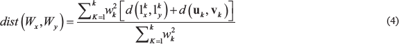
d i s t (W_{x}, W_{y}) = \frac{\sum_{K = 1}^{k} w_{k}^{2} [d (l_{x}^{k}, l_{y}^{k}) + d (u_{k}, v_{k})]}{\sum_{K = 1}^{k} w_{k}^{2}}

(4)

where the wavelet transforms of x and y are given by Wx(.) and Wy(.), respectively. Moreover, wk are the weights equal to the squared covariance explained by each axis, uk and vk are singular vectors satisfying variational properties lkx and lky are leading patterns. K represents the number of singular vectors used to capture the covariance in the data. In this work, we used K = 3 for all computations of dissimilarities. The full description of the dissimilarity measure used is provided by Aguiar-Conraria and Soares (2011).

We also measure the casual relationship among financial sectors comparing before and after the crisis in different frequencies, using wavelet-based Granger causality test, following Sharif et al. (2020). The test consists in applying discrete wavelet filtering to the original series and using the obtained components in frequencies (2–4 days, 4–8 days and so on) as inputs to a standard Granger (1969) test in a mean. Under the null hypothesis of no causality in the given frequency, the test statistic provides asymptotic chi-squared p-values. In this work, we use Maximal Overlap Discrete Wavelet Transform (MODWT) as the filtering technique. For a full description of this technique, refer to Percival and Mofjeld (1997).

Finally, in our main exercise, we use the wavelet-based VaR ratio shown in Rua and Nunes (2009). The VaR of a portfolio in the 1- confidence level can be defined in the following manner:

V a R (α) = I o Φ^{- 1} (1 - α) σ_{p}

(5)

where Io represents the initial investment, Φ-1(.) the cumulative distribution function of the standard normal, and σp the portfolio volatility. The VaR should be understood as the maximum loss to be expected of a portfolio with a certain level of confidence, being a widespread measure of risk.

Assuming a portfolio with n assets, its variance, can be computed as follows:

σ_{p}^{2} = \sum_{i = 1}^{n} w_{i}^{2} σ_{i}^{2} + \sum_{i = 1}^{n} \sum_{j = 1, j \neq i}^{n} w_{i} w_{j} cov (r_{i}, r_{j})

(6)

In Equation (6), and are the weight of asset in the portfolio, its volatility, and its return, respectively.

As one can see, the portfolio variance has two terms, the first formed by the variances of its components and the second formed by the connection between its components and the covariances. To study how the linkages between the components of a portfolio have evolved, following Rua and Nunes (2009), we examine the ratio between the variance of the portfolio computed with the full expression of Equation (6) and the variance computed excluding the covariance terms in Equation (6).

The intuition is that if this VaR ratio increases, it means there is an increase in co-movement of the components normalized by their variances, translating in more connection even when controlling by individual component risks.

However, we do not use time series expressions for computing Equation (6), but instead we use time-frequency domain wavelet-based analogue measures of variance and covariance. Thus, we use the Wavelet Power Spectrum and Cross-Wavelet Transform described in Equations (2) and (3), respectively. This procedure allows us to observe how the connections have changed in time and frequency through three dimensional maps.

Data Source

Our data are comprised of daily percent returns of G7 financial sector indices from 1 January 2015 to 16 October 2020. Namely, we use S&P/TSX Canadian Financials (Canada), CAC Financials (France), DAX Financial Services (Germany), FTSE Italia All Share Financials (Italy), Nikkei 500 other financial services (Japan), FTSE 350 Financial Services (UK), and S&P Financials (US) indices.

Figure 1.

Source: The authors.

All data have been gathered from Investing.com.

Results and Discussion

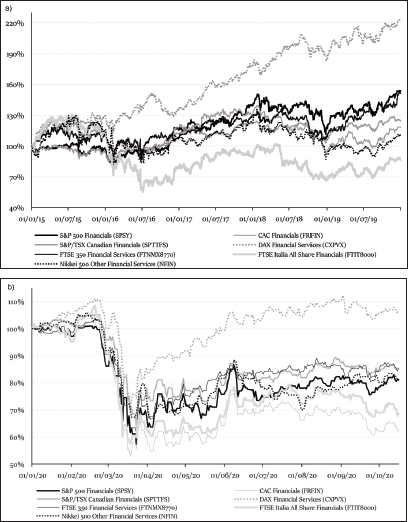
Figure 1 shows cumulative nominal return on financial sector indices in terms of the local investor´s currency, based on the daily time series for the end-of-day quote, from 1 January 2015 to 16 October 2020.

Over the period from 2015 to 2019—characterized by a period without crisis by National Bureau of Economic Research (NBER)—only the Italian banking sector recorded a cumulative loss of 13.2%, as a result of a downward trend during the mid-2015 period to mid-2016. The other banking indices showed cumulative gains, ranging from 9.7% in Japan to 123.1% in Germany. This German banking sector is the only one diverging from the others.

The cumulative return in the year 2020, however, suggests a pattern with very sharp accumulated declines from the second half of February, again with divergence from the German banking sector, from the second half of March 2020. DAX Financial Services is the only one that registered a cumulative return from 1 January 2020 to 16 October 2020, exceeding 5%.

Concerning these time series, they are not Gaussian but rather driven by Laplace and Generalized extreme value, among other PDFs. Moreover, Matos et al. (2019b) find that they share an equilibrium relationship so that they cannot move independently in the short- and long-run, and according to Matos et al. (2019a), those indices seem to be generated from a nonlinear and nonchaotic system, based on Brock, Dechert, Scheinkman (BDS) test and the Lyapunov exponent.

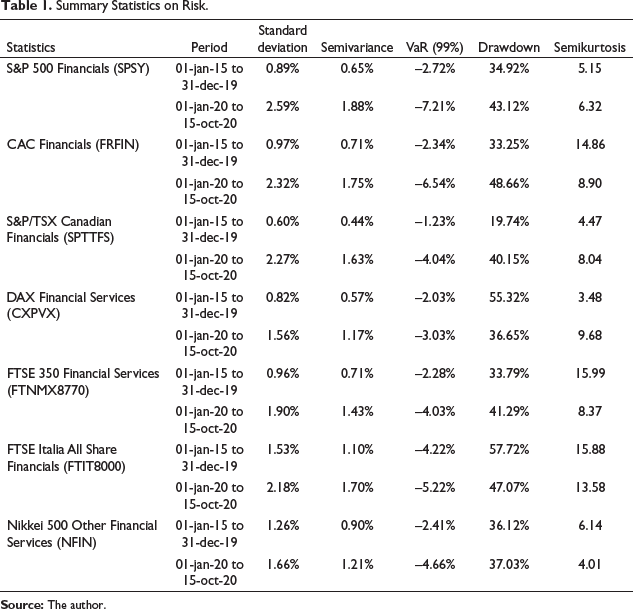
We report main statistics on risk in the Table 1.

The analysis of the standard deviation during the pre-pandemic period and during the pandemic suggests an increase in all G7 indices, and this relative increase is smaller in Japan and Italy, and higher in Canada and the USA. We find a similar pattern based on the semi-variance. Among the countries with the greatest increase in risk, only the USA was severely affected by cases and deaths by COVID-19. VaR obtained from the quantile function extracted from the best fitting distribution, following Matos et al. (2015) suggests that there are banking sectors with more comfortable risk management, as in Germany, while in the USA and France, this metric increased by more than 4% in the pandemic.

The analysis based on the drawdown shows a concern about the worst cumulative fall in the banking system in France, a country strongly affected by the deaths by COVID-19. There is also evidence of a reduction in the drawdown recorded in the pandemic compared to that seen in the period from 2019 to 2019 in Italy and Germany. The German banking sector showed the greatest increase in semi kurtosis, while the banking sectors in France, UK, Italy, and Japan had a reduction in this unilateral fourth-order moment.

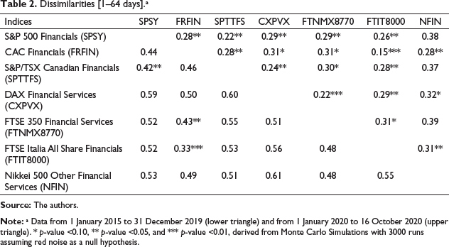
Concerning this concept of dissimilarity, given that we use the Hermitian angle, the highest value the distance can take is, while a value very close to zero means that two countries have a very similar wavelet transform, or they share the same high-power regions and also that their phases are aligned. In other words, the contribution of cycles at each frequency to the total variance is similar between both countries.

According to the dissimilarities reported in Table 2, considering the frequency from 1 to 64 days, in the pre-pandemic period, of the 21 possible pairwise combinations, only 3 were significant. In 2020, the pandemic seems to have intensified this metric of contagion. There are now 18 possible significant pairwise combinations. The only three non-significant combinations are associated with the banking sector in Japan, a country little affected by COVID-19. We may infer that in 2020, the ups and downs of each G7 banking cycle occur simultaneously in both countries, except for Japan versus UK, the USA and Canada. During the pre-pandemic period, the average dissimilarity was 0.51, while in 2020, the average was 0.30, a reduction of 42.1%.

Table 1.

Summary Statistics on Risk.

Statistics	Period	Standard deviation	Semivariance	VaR (99%)	Drawdown	Semikurtosis
S&P 500 Financials (SPSY)	01-jan-15 to 31-dec-19	0.89%	0.65%	-2.72%	34.92%	5.15
S&P 500 Financials (SPSY)	01-jan-20 to 15-oct-20	2.59%	1.88%	-7.21%	43.12%	6.32
CAC Financials (FRFIN)	01-jan-15 to 31-dec-19	0.97%	0.71%	-2.34%	33.25%	14.86
CAC Financials (FRFIN)	01-jan-20 to 15-oct-20	2.32%	1.75%	-6.54%	48.66%	8.90
S&P/TSX Canadian Financials (SPTTFS)	01-jan-15 to 31-dec-19	0.60%	0.44%	-1.23%	19.74%	4.47
S&P/TSX Canadian Financials (SPTTFS)	01-jan-20 to 15-oct-20	2.27%	1.63%	-4.04%	40.15%	8.04
DAX Financial Services (CXPVX)	01-jan-15 to 31-dec-19	0.82%	0.57%	-2.03%	55.32%	3.48
DAX Financial Services (CXPVX)	01-jan-20 to 15-oct-20	1.56%	1.17%	-3.03%	36.65%	9.68
FTSE 350 Financial Services (FTNMX8770)	01-jan-15 to 31-dec-19	0.96%	0.71%	-2.28%	33.79%	15.99
FTSE 350 Financial Services (FTNMX8770)	01-jan-20 to 15-oct-20	1.90%	1.43%	-4.03%	41.29%	8.37
FTSE Italia All Share Financials (FTIT8000)	01-jan-15 to 31-dec-19	1.53%	1.10%	-4.22%	57.72%	15.88
FTSE Italia All Share Financials (FTIT8000)	01-jan-20 to 15-oct-20	2.18%	1.70%	-5.22%	47.07%	13.58
Nikkei 500 Other Financial Services (NFIN)	01-jan-15 to 31-dec-19	1.26%	0.90%	-2.41%	36.12%	6.14
Nikkei 500 Other Financial Services (NFIN)	01-jan-20 to 15-oct-20	1.66%	1.21%	-4.66%	37.03%	4.01

Source: The author.

Table 2.

Dissimilarities [1–64 days].^a

Indices	SPSY	FRFIN	SPTTFS	CXPVX	FTNMX8770	FTIT8000	NFIN
S&P 500 Financials (SPSY)		0.28**	0.22**	0.29**	0.29**	0.26**	0.38
CAC Financials (FRFIN)	0.44		0.28**	0.31*	0.31*	0.15***	0.28**
S&P/TSX Canadian Financials (SPTTFS)	0.42**	0.46		0.24**	0.30*	0.28**	0.37
DAX Financial Services (CXPVX)	0.59	0.50	0.60		0.22***	0.29**	0.32*
FTSE 350 Financial Services (FTNMX8770)	0.52	0.43**	0.55	0.51		0.31*	0.39
FTSE Italia All Share Financials (FTIT8000)	0.52	0.33***	0.53	0.56	0.48		0.31**
Nikkei 500 Other Financial Services (NFIN)	0.53	0.49	0.51	0.61	0.48	0.55

Source: The authors.

Note: ^a Data from 1 January 2015 to 31 December 2019 (lower triangle) and from 1 January 2020 to 16 October 2020 (upper triangle). * p-value <0.10, ** p-value <0.05, and *** p-value <0.01, derived from Monte Carlo Simulations with 3000 runs assuming red noise as a null hypothesis.

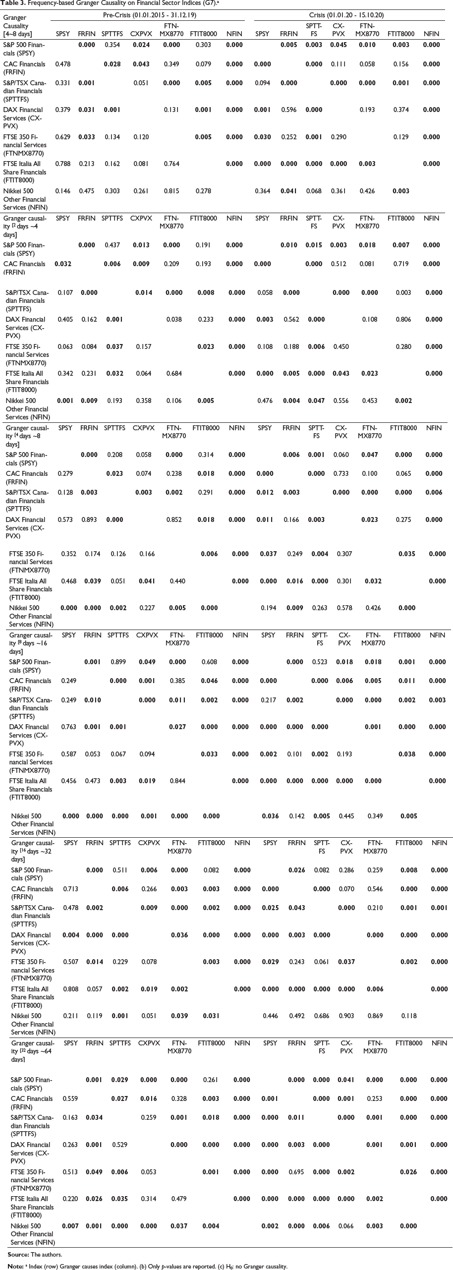
In terms of causality, the results of the original test (Table 3) suggest that among the 42 possible combinations involving the G7 banking systems, there are 23 combinations without causality in the pre-pandemic period, while during the pandemic, there are only 14 without causality. Only in the frequency of 16 ∼ 32 days, we find more causalities in the period from 2015 to 2019, than in 2020. It is important to highlight that the banking contagion in 2020 measured by causality seems to be stronger and more widespread in the lowest frequency, 32–64 days. We find 39 combinations with significant causality at 5%, among 42 possible ones. Due to the fast reaction of the financial system, the most relevant causality is based on the highest frequency, 2–4 days. Japanese banking cycles have always been influenced by banking cycles in other G7 countries, before and during the pandemic. The interesting difference is the increase of the predictive power of banking cycles in the USA and especially in the Italian banking system. In the pre-pandemic period, Italian banking cycles were able to anticipate only Canadian and Japanese cycles. During the pandemic, Italian cycles came to be useful in predicting banking cycles in all other G7 economies. We remember that Italy was the first developed economy to suffer more strongly from the effects of COVID-19, in cases and deaths.

Finally, we know that the portfolio variance can be decomposed in two factors linked to variance and covariance of pairs of assets. The ratio between the variances of the portfolio with and without assuming co-movement brings information about how much linkage there is among the assets comprising the portfolio. In other words, analysing how this ratio evolve in the time-frequency plain can show if there is evidence of contagion (increase in linkage) among the components of the portfolio. Figure 2 reports the squared VaR ratio taking into account an equally weighted portfolio of G7 financial sector indices, with and without co-movements. Numerically, before the pandemic period, the average of ratio (not squared) was 1.70, while throughout the year 2020 until 15 October this average was 2.05.

Table 3.

Frequency-based Granger Causality on Financial Sector Indices (G7).^a

Granger Causality [4∼8 days]	Pre-Crisis (01.01.2015 - 31.12.19)							Crisis (01.01.20 - 15.10.20)
Granger Causality [4∼8 days]	SPSY	FRFIN	SPTTFS	CXPVX	FTNMX8770	FTIT8000	NFIN	SPSY	FRFIN	SPTTFS	CXPVX	FTNMX8770	FTIT8000	NFIN
S&P 500 Financials (SPSY)		0.000	0.354	0.024	0.000	0.303	0.000		0.005	0.003	0.045	0.010	0.003	0.000
CAC Financials (FRFIN)	0.478		0.028	0.043	0.349	0.079	0.000	0.000		0.000	0.111	0.058	0.156	0.000
S&P/TSX Canadian Financials (SPTTFS)	0.331	0.001		0.051	0.000	0.005	0.000	0.094	0.000		0.000	0.000	0.001	0.000
DAX Financial Services (CXPVX)	0.379	0.031	0.001		0.131	0.001	0.000	0.001	0.596	0.000		0.193	0.374	0.000
FTSE 350 Financial Services (FTNMX8770)	0.629	0.033	0.134	0.120		0.005	0.000	0.030	0.252	0.001	0.290		0.129	0.000
FTSE Italia All Share Financials (FTIT8000)	0.788	0.213	0.162	0.081	0.764		0.000	0.000	0.000	0.000	0.000	0.003		0.000
Nikkei 500 Other Financial Services (NFIN)	0.146	0.475	0.303	0.261	0.815	0.278		0.364	0.041	0.068	0.361	0.426	0.003
Granger causality [² days ∼4 days]	SPSY	FRFIN	SPTTFS	CXPVX	FTNMX8770	FTIT8000	NFIN	SPSY	FRFIN	SPTTFS	CXPVX	FTNMX8770	FTIT8000	NFIN
S&P 500 Financials (SPSY)		0.000	0.437	0.013	0.000	0.191	0.000		0.010	0.015	0.003	0.018	0.007	0.000
CAC Financials (FRFIN)	0.032		0.006	0.009	0.209	0.193	0.000	0.000		0.000	0.512	0.081	0.719	0.000
Granger Causality [2∼4 days]	Pre-Crisis (01.01.2015 - 31.12.19)							Crisis (01.01.20 - 15.10.20)
Granger Causality [2∼4 days]	SPSY	FRFIN	SPTTFS	CXPVX	FTNMX8770	FTIT8000	NFIN	SPSY	FRFIN	SPTTFS	CXPVX	FTNMX8770	FTIT8000	NFIN
S&P/TSX Canadian Financials (SPTTFS)	0.107	0.000		0.014	0.000	0.008	0.000	0.058	0.000		0.000	0.000	0.003	0.000
DAX Financial Services (CXPVX)	0.405	0.162	0.001		0.038	0.233	0.000	0.003	0.562	0.000		0.108	0.806	0.000
FTSE 350 Financial Services (FTNMX8770)	0.063	0.084	0.037	0.157		0.023	0.000	0.108	0.188	0.006	0.450		0.280	0.000
FTSE Italia All Share Financials (FTIT8000)	0.342	0.231	0.032	0.064	0.684		0.000	0.000	0.005	0.000	0.043	0.023		0.000
Nikkei 500 Other Financial Services (NFIN)	0.001	0.009	0.193	0.358	0.106	0.005		0.476	0.004	0.047	0.556	0.453	0.002
Granger causality [⁴ days ∼8 days]	SPSY	FRFIN	SPTTFS	CXPVX	FTNMX8770	FTIT8000	NFIN	SPSY	FRFIN	SPTTFS	CXPVX	FTNMX8770	FTIT8000	NFIN
S&P 500 Financials (SPSY)		0.000	0.208	0.058	0.000	0.314	0.000		0.006	0.001	0.060	0.047	0.000	0.000
CAC Financials (FRFIN)	0.279		0.023	0.074	0.238	0.018	0.000	0.000		0.000	0.733	0.100	0.065	0.000
S&P/TSX Canadian Financials (SPTTFS)	0.128	0.003		0.003	0.002	0.291	0.000	0.012	0.003		0.000	0.000	0.000	0.006
DAX Financial Services (CXPVX)	0.573	0.893	0.000		0.852	0.018	0.000	0.011	0.166	0.003		0.023	0.275	0.000
Granger Causality [4∼8 days]	Pre-Crisis (01.01.2015 - 31.12.19)							Crisis (01.01.20 - 15.10.20)
Granger Causality [4∼8 days]	SPSY	FRFIN	SPTTFS	CXPVX	FTNMX8770	FTIT8000	NFIN	SPSY	FRFIN	SPTTFS	CXPVX	FTNMX8770	FTIT8000	NFIN
FTSE 350 Financial Services (FTNMX8770)	0.352	0.174	0.126	0.166		0.006	0.000	0.037	0.249	0.004	0.307		0.035	0.000
FTSE Italia All Share Financials (FTIT8000)	0.468	0.039	0.051	0.041	0.440		0.000	0.000	0.016	0.000	0.301	0.032		0.000
Nikkei 500 Other Financial Services (NFIN)	0.000	0.000	0.002	0.227	0.005	0.000		0.194	0.009	0.263	0.578	0.426	0.000
Granger causality [⁸ days ∼16 days]	SPSY	FRFIN	SPTTFS	CXPVX	FTNMX8770	FTIT8000	NFIN	SPSY	FRFIN	SPTTFS	CXPVX	FTNMX8770	FTIT8000	NFIN
S&P 500 Financials (SPSY)		0.001	0.899	0.049	0.000	0.608	0.000		0.000	0.523	0.018	0.018	0.001	0.000
CAC Financials (FRFIN)	0.249		0.000	0.001	0.385	0.046	0.000	0.000		0.000	0.006	0.005	0.011	0.000
S&P/TSX Canadian Financials (SPTTFS)	0.249	0.010		0.000	0.011	0.002	0.000	0.217	0.002		0.000	0.000	0.002	0.003
DAX Financial Services (CXPVX)	0.763	0.001	0.001		0.027	0.000	0.000	0.000	0.000	0.000		0.001	0.000	0.000
FTSE 350 Financial Services (FTNMX8770)	0.587	0.053	0.067	0.094		0.033	0.000	0.002	0.101	0.002	0.193		0.038	0.000
FTSE Italia All Share Financials (FTIT8000)	0.456	0.473	0.003	0.019	0.844		0.000	0.000	0.000	0.000	0.000	0.000		0.000
Granger Causality [4∼8 days]	Pre-Crisis (01.01.2015 - 31.12.19)							Crisis (01.01.20 - 15.10.20)
Granger Causality [4∼8 days]	SPSY	FRFIN	SPTTFS	CXPVX	FTNMX8770	FTIT8000	NFIN	SPSY	FRFIN	SPTTFS	CXPVX	FTNMX8770	FTIT8000	NFIN
Nikkei 500 Other Financial Services (NFIN)	0.000	0.000	0.000	0.001	0.000	0.000		0.036	0.142	0.005	0.445	0.349	0.005
Granger causality [16 days ∼32 days]	SPSY	FRFIN	SPTTFS	CXPVX	FTNMX8770	FTIT8000	NFIN	SPSY	FRFIN	SPTTFS	CXPVX	FTNMX8770	FTIT8000	NFIN
S&P 500 Financials (SPSY)		0.000	0.511	0.006	0.000	0.082	0.000		0.026	0.082	0.286	0.259	0.008	0.000
CAC Financials (FRFIN)	0.713		0.006	0.266	0.003	0.003	0.000	0.000		0.000	0.070	0.546	0.000	0.000
S&P/TSX Canadian Financials (SPTTFS)	0.478	0.002		0.009	0.000	0.002	0.000	0.025	0.043		0.000	0.210	0.001	0.001
DAX Financial Services (CXPVX)	0.004	0.000	0.000		0.036	0.000	0.000	0.000	0.003	0.000		0.000	0.000	0.000
FTSE 350 Financial Services (FTNMX8770)	0.507	0.014	0.229	0.078		0.003	0.000	0.029	0.243	0.061	0.037		0.002	0.000
FTSE Italia All Share Financials (FTIT8000)	0.808	0.057	0.002	0.019	0.002		0.000	0.000	0.000	0.000	0.000	0.006		0.000
Nikkei 500 Other Financial Services (NFIN)	0.211	0.119	0.001	0.051	0.039	0.031		0.446	0.492	0.686	0.903	0.869	0.118
Granger causality [³² days ∼64 days]	SPSY	FRFIN	SPTTFS	CXPVX	FTNMX8770	FTIT8000	NFIN	SPSY	FRFIN	SPTTFS	CXPVX	FTNMX8770	FTIT8000	NFIN
Granger Causality [32∼64 days]	Pre-Crisis (01.01.2015 - 31.12.19)							Crisis (01.01.20 - 15.10.20)
Granger Causality [32∼64 days]	SPSY	FRFIN	SPTTFS	CXPVX	FTNMX8770	FTIT8000	NFIN	SPSY	FRFIN	SPTTFS	CXPVX	FTNMX8770	FTIT8000	NFIN
S&P 500 Financials (SPSY)		0.001	0.029	0.000	0.000	0.261	0.000		0.000	0.000	0.041	0.000	0.000	0.000
CAC Financials (FRFIN)	0.559		0.027	0.016	0.328	0.003	0.000	0.001		0.000	0.001	0.253	0.000	0.000
S&P/TSX Canadian Financials (SPTTFS)	0.163	0.034		0.259	0.001	0.018	0.000	0.000	0.011		0.000	0.001	0.000	0.000
DAX Financial Services (CXPVX)	0.263	0.001	0.529		0.000	0.000	0.000	0.000	0.003	0.000		0.001	0.001	0.000
FTSE 350 Financial Services (FTNMX8770)	0.513	0.049	0.006	0.053		0.001	0.000	0.000	0.695	0.000	0.002		0.026	0.000
FTSE Italia All Share Financials (FTIT8000)	0.220	0.026	0.035	0.314	0.479		0.000	0.000	0.000	0.000	0.000	0.002		0.000
Nikkei 500 Other Financial Services (NFIN)	0.007	0.001	0.000	0.000	0.037	0.004		0.002	0.000	0.006	0.066	0.003	0.000

Source: The authors.

Note: ^a Index (row) Granger causes index (column). (b) Only p-values are reported. (c) H₀: no Granger causality.

Considering the height of the pandemic (February and March 2020), this average was 2.23. In both cases, there are increases of 21% and 31% in relation to the period that anticipated the pandemic.

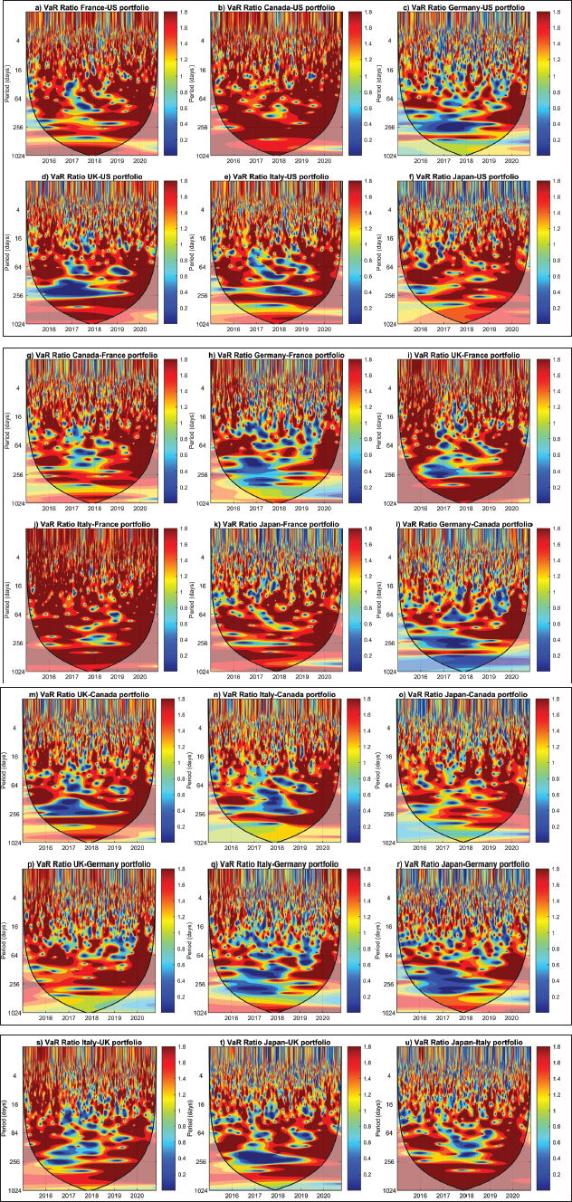
In the appendix, Figure A1 reports the 21 possible pairwise combinations with the G7 financial indices. In most of them, the region characterized by a frequency of 16 to 256 days is predominantly dark red, which suggests a VaR ratio greater than 1, that is, stronger contagion between both banking systems. This is particularly true during the pandemic period. Some of the main highlights are the following pairwise: USA and France, USA and Canada, and Canada and France. The highest contagion is found in the Italian and French banking systems, countries severely affected by deaths by COVID-19, while the least contagion, measured by the VaR ratio, is evident between Japan and Germany, countries least affected by the first wave of COVID-19.

Figure 2.

Source: The authors.

Conclusion and Managerial Implications

We add to the debate on G7 banking contagion during this pandemic based on comparison of risk metrics, dissimilarities, frequency-based Granger causalities, and VaR ratio.

Some of our main conclusions suggest an increase in contagion and the effect on risk management, mainly involving the countries most affected by the pandemic. The VaR-based analysis suggests that there are banking sectors with more comfortable risk management, as in Germany, while in the USS and France, this metric increased by more than 4% in the pandemic. According to the wavelet dissimilarities, the pandemic seems to have intensified this metric of contagion, and the non-significant combinations are associated with the banking sector in Japan, a country little affected by COVID-19. We also may highlight the increase in the predictive relevance of Italian banking cycles in during the pandemic. Based on VaR ratio analysis, we find a stronger banking contagion during the pandemic period, especially considering the height of the pandemic (February and March 2020). The highest contagion is found in the Italian and French banking systems, countries severely affected by deaths by COVID-19, while the least contagion, measured by the VaR ratio, is evident between Japan and Germany, countries least affected by the first wave of COVID-19.

We believe that the systematic contagion effects present in these markets during this health crisis could not have been necessarily reduced by further banking regulatory measures such as increased capital requirements. However, there is a gain for researchers and policymakers to consider how does it work the transmission of business cycles between each pair of banking systems or even considering a small group of countries. It seems useful to identify which banking system can act as a leader in the group of synchronized countries. In this context, our main findings are aligned to Matos et al. (2019b) and they can shed light on this discussion on business cycle synchronization and trade. We also claim that our findings are useful to draw public policies to safeguard financial stability and to analyse the timing of the impact of the pandemic crises in each G7 banking sector.

Furthermore, from a practical point of view, our findings have managerial implications in informing asset managers and banking sector investors decisions alike; for instance, we have evidenced the fact that banking sectors have had much more similar spectrums during the COVID-19 pandemic, indicating increased dynamic correlations in each time horizon, and, thus, less benefits of geographic diversification inside the banking sector during highly stressful moments.

Similar use can be drawn for the Granger causality analysis, which showed a predictability increase, mainly from sectors of countries under high stress, like Italy and the USA to the others. This behaviour suggests possible suitability of the returns of banking sectors in highly stressed markets as variables in asset pricing models used for asset managers and other finance practitioners.

Finally, the provided pairwise time-frequency maps of VaR ratios indicate that in the long run, represented by components at frequencies of 16–256 days, there is evidence of historically high linkages between banking sectors, one that is increased considerably during this pandemic. Thus, the geographic diversification provided in a banking portfolio of G7 countries is shown to be more important to protect for the short-run minded investor. Another use of the VaR ratios maps is to indicate the less connected pairwise of banking sectors in a time-frequency manner, hinting best candidates for a portfolio formation given the time horizon interest of the investor.

Appendix A

Figure A1.

Source: The authors.

Footnotes

Suggestion for Future Research

The present work has been focused on the linkages between returns, but could well have used metrics of risks, as volatilities or VaR itself, as the variables of interest. This approach could yield some new perspectives, as discussed in . However, we have not added other metrics of risk as the variables of interest in this work because of the space needed. Thus, we understand this would be a natural extension to be addressed in future research.

We also understand that there are other groups of countries to be addressed, to which the framework here employed could bring some new results. Specifically, an interesting extension of this work could be obtained focusing on relevant emerging markets, for instance, the BRICS.

Acknowledgement

The authors are grateful to the anonymous referees of the journal for their extremely useful suggestions to improve the quality of the article. Usual disclaimers apply.

Declaration of Conflicting Interests

The authors declared no potential conflicts of interest with respect to the research, authorship and/or publication of this article.

Funding

The authors received no financial support for the research, authorship and/or publication of this article.

ORCID iDs

Antonio Costa

Cristiano da Silva

References

Aguiar-Conraria

, & Soares

(2011). Business cycle synchronization and the Euro: A wavelet analysis. Journal of Macroeconomics , 33, 477–489.

Aguiar-Conraria

, Martins

, & Soares

(2018). Estimating the Taylor rule in the time-frequency domain. Journal of Macroeconomics , 57, 122–137.

Aharony

, & Swary

(1983). Contagion effects of bank failures: Evidence from capital markets. The Journal of Business , 56, 305–322.

Akhtaruzzaman

, Boubaker

, & Sensoy

(2021). Financial contagion during COVID–19 crisis. Finance Research Letters , 38, 101604.

Benhmad

(2013). Dynamic cyclical comovements between oil prices and US GDP: A wavelet perspective. Energy Policy , 57, 141–151

Bordo

, Eichengreen

, Klingebiel

, & Martinez-Peria

M. S.

(2001). Is the crisis problem growing more severe? Economic Policy , 16, 51–82.

Calvo

G. A.

, & Mendoza

E. G.

(2000). Rational contagion and the globalization of securities markets. Journal of International Economics , 51(1), 79–113.

Costa

, da Silva

, & Matos

(2020). Examining international financial sector contagion during COVID-19 pandemics with Wavelet and FR statistic (Working Paper). CAEN/UFC.

Diebold

F. X.

, & Yilmaz

(2009). Measuring financial asset return and volatility spillovers, with application to global equity markets. Economic Journal , 119, 158–171.

10.

Diebold

F. X.

, & Yılmaz

(2012). Better to give than to receive: Predictive directional measurement of volatility spillovers. International Journal of Forecasting , 28, 57–66.

11.

Dungey

, & Gajurel

(2015). Contagion and banking crisis—International evidence for 2007–2009. Journal of Banking and Finance , 60, 271–283.

12.

Elliott

, Golub

, & Jackson

M. O.

(2014). Financial networks and contagion. American Economic Review , 104(10), 3115–53.

13.

Engle

(2002). Dynamic conditional correlation. Journal of Business and Economic Statistics , 20, 339–350.

14.

Filho

J. J.

, Matos

, & Fonseca

(2020). The role of contagion and integration in risk management measures. Global Business Review . https://doi.org/10.1177/0972150920933857

15.

Forbes

, & Rigobon

(2002). No contagion, only interdependence: Measuring stock market co-movements. Journal of Finance , 57, 2223–2261.

16.

Gallegati

(2012). A wavelet-based approach to test for financial market contagion. Computational Statistics and Data Analysis , 56, 3491–3497.

17.

Gamba-Santamaria

, Gomez-Gonzalez

J. E.

, Hurtado-Guarin

J. L.

, & Melo-Velandia

L. F.

(2017). Stock market volatility spillovers: Evidence for Latin America. Finance Research Letters , 20, 207–216.

18.

Granger

C. W.

(1969). Investigating causal relations by econometric models and cross-spectral methods. Econometrica , 37, 424–438.

19.

Goodell

(2020). COVID-19 and finance: Agenda for future research. Finance Research Letters , 35, 101512.

20.

Grossmann

, & Morlet

(1984). Decomposition of Hardy functions into square integrable wavelets of constant shape. SIAM Journal on Mathematical Analysis , 15, 723–736.

21.

Hung

N. T.

(2019). Spillover effects between stock prices and exchange rates for the central and eastern European countries. Global Business Review . https://doi.org/10.1177/0972150919869772

22.

Jokipii

, & Lucey

(2007). Contagion and interdependence: Measuring CEE banking sector co-movements. Economic Systems , 31(1), 71–96.

23.

Kaminsky

G. L.

, & Reinhart

C. M.

(2000). On crises, contagion, and confusion. Journal of International Economics , 51(1), 145–168.

24.

Kaminsky

G. L.

, & Reinhart

C. M.

(2002). Financial markets in times of stress. Journal of Development Economics , 69(2), 451–470.

25.

Laeven

, & Valencia

(2013). Systemic banking crises database. IMF Economic Review , 61, 225–270.

26.

Matos

, Jucá

, Cruz

, & Macedo

(2015). BRIC’s risk management based on an innovative VaR. The Empirical Economics Letters , 14, 697–704.

27.

Matos

, Benegas

, & Costa

(2019a). Chaos in the world banking sector? Nonlinear asset pricing models matter (Working Paper). CAEN/UFC.

28.

Matos

, da Silva

, & Oliveira

(2019b). Worldwide banking cycle synchronization (Working Paper)CAEN/UFC.

29.

Matos

, Costa

, & da Silva

(2021). COVID-19, stock market and sectoral contagion in US: A time-frequency analysis. Research in International Business and Finance , 57, 101400.

30.

Mensi

, Nekhili

, Vo Vinh

, Suleman

, & Hoon Kang

(2020). Asymmetric volatility connectedness among U.S. stock sectors. North American Journal of Economics and Finance . https://doi.org/10.1016/j.najef.2020.101327

31.

Mink

(2015). Measuring stock market contagion: local or common currency returns? Emerging Markets Review , 22, 18–24.

32.

Moser

(2003). What is international financial contagion? International Finance , 6(2), 157–178.

33.

OECD. (2012, June). Financial contagion in the era of globalised banking? (No. 14). OECD Economics Department Policy Notes.

34.

Pavlova

, & Rigobon

(2008). The role of portfolio constraints in the international propagation of shocks. The Review of Economic Studies , 75(4), 1215–1256.

35.

Percival

, & Mofjeld

(1997). Analysis of subtidal coastal sea level fluctuations using wavelets. Journal of the American Statistical Association , 92, 868–880.

36.

Rajwani

, & Kumar

(2016). Asymmetric dynamic conditional correlation approach to financial contagion: A study of Asian markets. Global Business Review , 17, 1339–1356.

37.

Rajwani

, & Kumar

(2019). Measuring dependence between the USA and the Asian economies: A time-varying copula approach. Global Business Review , 20, 962–980.

38.

Rigobon

(2019). Contagion, spillover, and interdependence. Economía , 19(2), 69–100.

39.

Rua

(2012). Wavelets in economics . Economic Bulletin and Financial Stability Report (Articles, 8). Banco de Portugal, Economics and Research Department.

40.

Rua

, & Nunes

(2009). International comovement of stock market returns: A wavelet analysis. Journal of Empirical Finance , 16, 632–639.

41.

Sharif

, Aloui

, & Yarovaya

(2020). COVID-19 pandemic, oil prices, stock market, geopolitical risk and policy uncertainty nexus in the US economy: Fresh evidence from the wavelet based approach. International Review of Financial Analysis . https://doi.org/10.1016/j.irfa.2020.101496

42.

Wang

G. J.

, Xie

, Lin

, & Stanley

H. E.

(2017). Stock market contagion during the global financial crisis: A multiscale approach. Finance Research Letters , 22, 163–168.

On the Risk-based Contagion of G7 Banking System and the COVID-19 Pandemic

Abstract

Keywords

Introduction

Literature Review

Research Objectives and Rationale

Methodology

Data Source

Results and Discussion

Summary Statistics on Risk.

Dissimilarities [1–64 days].a

Frequency-based Granger Causality on Financial Sector Indices (G7).a

Conclusion and Managerial Implications

Appendix A

Footnotes

Suggestion for Future Research

Acknowledgement

Declaration of Conflicting Interests

Funding

ORCID iDs

References

Dissimilarities [1–64 days].^a

Frequency-based Granger Causality on Financial Sector Indices (G7).^a