
Abstract
In this article, we tried to investigate the trade flow of India with the rest of the Brazil, Russia, India, China and South African (BRICS) countries. To do this, we augmented the gravity model of trade by incorporating time-invariant variables such as per capita gross domestic product (PCGDP), distance, language, etc. We used a panel data econometric model (i.e., pooled ordinary least squares—OLS, fixed effect model) and Poisson–Pseudo Maximum Likelihood (PPML) methods. The sample size consists of BRICS countries and top merchandise export partner countries of India over the period of 2001–2016. The empirical results revealed that the traditional arguments of the gravity model in the context of India are valid. However, as distance increases, export of goods is adversely affected due to a higher trade cost. Moreover, common official language and common border positively influence trade. In addition, evidence on marginal trade creation (21% above the normal level) has been observed. The study suggests that the Indian government should negotiate trade dialogues to resolve trade barriers and market access hurdles among the BRICS countries. This will increase exports among nations. Thus, trade relationship among the BRICS members needs to be addressed on a priority basis.
Introduction
The world economic growth is highly dependent on the growth of developing counties’ economic growth (WEO, 2018). The developing countries are growing at 4.7 per cent economic growth, while the world is growing on an average of 3.7 per cent economic growth. In addition, the BRICS economies were found to grow at 3.56 per cent on an average in 2017. This is also reflected by the BRICS economic bloc. The term BRICS was coined by O’Neill (2001). His study highlighted the term of future leading economies in the world. Thus, this becomes a strong proposition of foundation of the BRICS economic bloc. It came into effect since 2009 when the first summit was held in Yekaterinburg, Russia. Moreover, the 10th summit has been held in Johannesburg, South Africa, 2018, so far.
The BRIC acronym, which stands for Brazil, Russia, India and China, was introduced by O’Neill (2001). Later on, South Africa was added in 2010 and the term became BRICS. In Sachs’s papers, it was predicted that over the next 50 years, the BRIC economies would become the major economic forces in the world economy. They have also predicted that by 2050, the only existing industrialized/developed economies among the six largest global economies would be the USA, Japan and BRIC countries in terms of the US dollar (Government of India, 2012). In addition, China accessed the WTO in 2001; Russia accessed the WTO in 2010; and Brazil, India and South Africa are WTO founding members since 1995. Besides, the BRICS economies might influence WTO negotiation by shaping the global trade agenda. Usually, developed countries have an influence on WTO negotiations, but since the BRICS inception, developing counties’ voices became strong. In addition, in 2017, the global trade shares of countries are as follows: global export share of China (12.8%); Russia (2%); India (1.7%); and Brazil (1.2%); while of China stands at 10.2%); India 2.5%; Russia 1.3%; and Brazil 0.9%) in terms of global import share as per WTO (2018).
Traditionally, trade is regarded as an engine of growth, leading to development in general. Trade generally improves productivity through specialization, and then by means of trade creation (TC) and trade diversion (TD) effects, the welfare of the trading countries goes up. This idea gets nicely reflected in the acceptance of globalization across the globe. it is undeniable that counties around the world would try to appropriate the gains revealed by an institutional transaction of goods and services. Following such arguments, different trade associations and trade blocs are formed. The North American Free Trade Agreement (NAFTA), the South Asian Free Trade Area (SAFTA), Association of Southeast Asian Nations (ASEAN) and BRICS are some of them. Though different trade blocs have their own agenda and strategies, their main motive is to ensure the highest trade volume among the member countries. BRICS is no exception. In this article, we would focus on BRICS and its impacts.
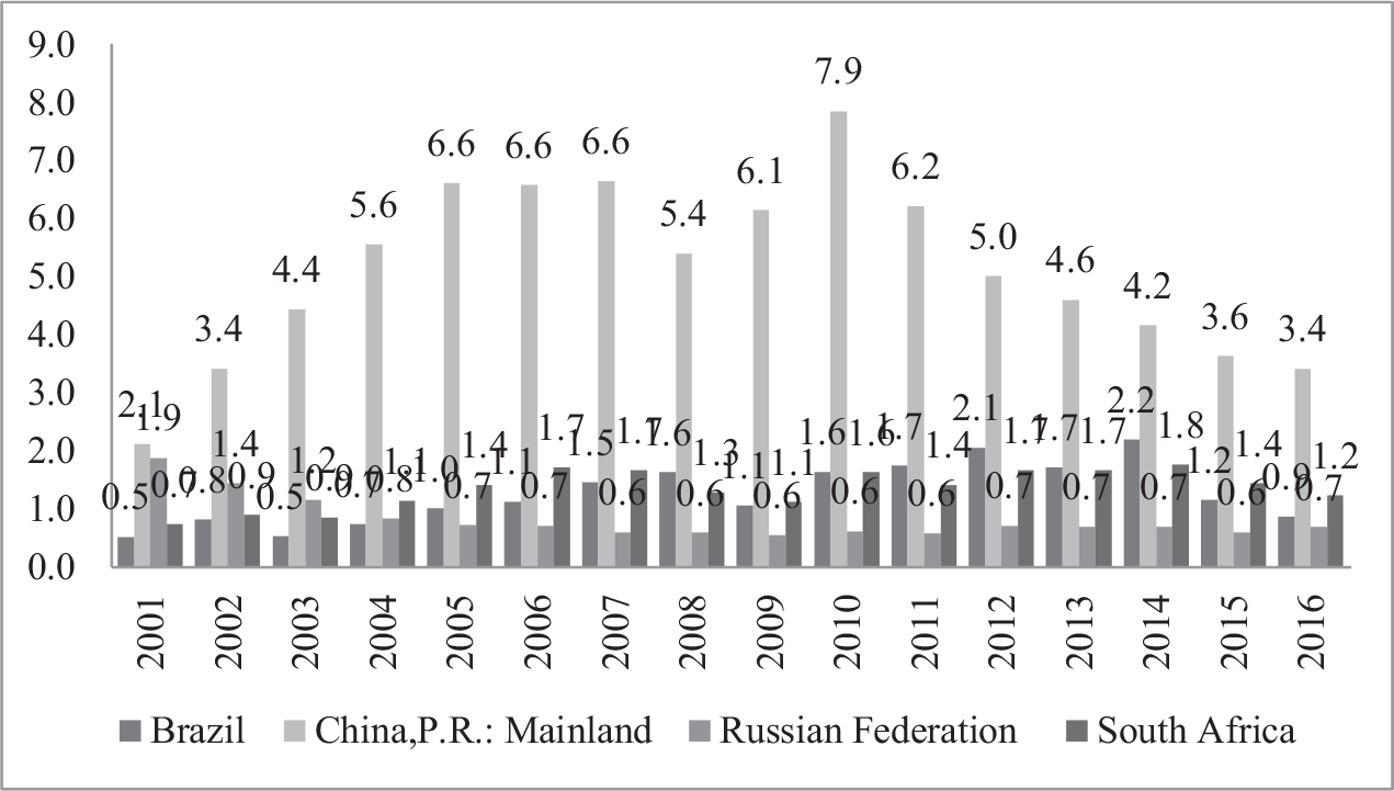
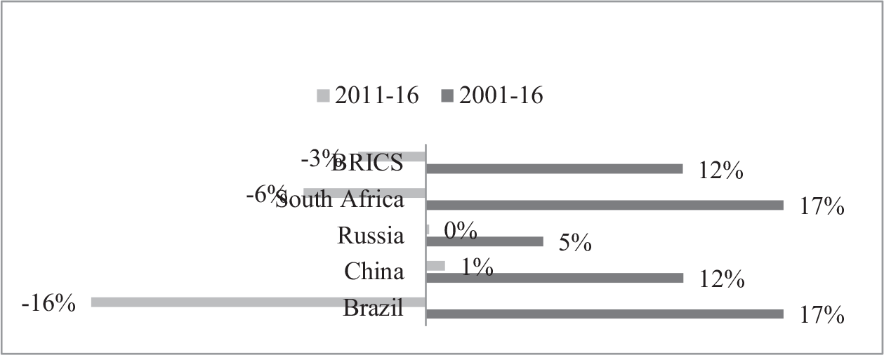
Furthermore, BRICS countries trade share in world trade has been dramatically increased in the recent past. In particular, trade between India and the rest of BRICS countries increased but not as expected. The export share of rest of BRICS countries in the Indian merchandise export has increased from 5.2 per cent to 6.3 per cent during 2001–2016 (see Figure 1). Figure 2 depicts compounded annual growth rate of India’s export to the rest of BRICS countries at 12 per cent. In addition, in the past 6 years, merchandise export declined by 3 per cent during the period 2011–2016. Figure 1 shows the export share of BRICS countries at the country level. It is revealed that China is an active export destination ranging from 2.1 per cent to 3.4 per cent during 2001–2016. However, Brazil, Russia and South Africa’s export share in Indian export is not more than 2.2 per cent. Furthermore, the export growth of India with Brazil, China and South Africa has witnessed rapid growth at 17 per cent, 12 per cent and 17 per cent, respectively. But In the case of Russia, it is only 5 per cent. However, in the recent period, India’s export to Brazil and South Africa declined sharply by 16 per cent and 6 per cent, respectively. In addition, India’s export growth to China increased by 1 per cent, while Russia showed no improvement.
The present study is an attempt to analyse the trade flow of India with the rest of BRICS countries and major trading partner countries over the period 2001–2016. To analyse the trade flow, the gravity model of trade has been employed. Furthermore, the study also investigates the TC (TD) effect as developed by Viner (1950). Time-invariant variable, that is, distance, the common official language, common border, multilateral resistance term [MRTs]/fixed effect model) has been included within the model. The MRTs have been included to control the unobserved heterogeneity within the model.
There are few studies that attempt to use the gravity model of trade in case of BRICS countries, for example, Mishra et al. (2015), Rasoulinezhad and Jabalameli (2018a, b), and Kubendran (2020). Although none of the studies tried to analyse the extension of Viner (1950) approach, this study fills the gap. We use the Free Trade Agreement (FTA) approach as used by Yang and Martinez-Zarzoso (2014), Kahouli and Maktouf (2013, 2015) and Khurana and Nauriyal (2017) to assess the export performance of the BRICS economic bloc.
The rest of the article is organized as follows: the second section talks about the review of the literature, which describes the origin of the gravity model along with empirical literature. the third section discusses our model specification. The fourth section presents the basic results of the article followed by discussion. Finally, the fifth section concludes the article with policy implications.
Review of Literature
Theoretical Framework: Intuitive Gravity Model
The notion of the gravity model of trade comes from universal gravitation law of Newton (1687). The theory says that the gravitational force is an attraction between two points. It is directly related to the multiple of their masses and negatively related to the square of the distance between their centres. In Equation (1), GFij illustrates that gravitational force between i and j point equals to the multiple of their masses (mimj) and negatively related to the square of their distance (d2ij).

In Equation (2), Tij states that gravitational force between i and j countries’ economic size (GDP) is equal to the multiple of their economic size (GDP) and negatively related to the bilateral distance (Dij).

In other words, trade is positively related to their product of economic mass and negatively related to trade cost (distance). As the economic mass of countries increases, trade also increases. In contrast, as trade cost (distance) increases, trade also decreases. The Tinbergen (1962) and Poyhonen (1963) applied the gravity model on trade flow analysis in international trade. The gravity model became more popular, and it is also called as a ‘workhorse’ model to analyse the effect of policy variables of trade and integration. Economists often analyse different versions of the gravity model of trade such as augmented gravity model, structural gravity model, etc.
Theoretical Gravity Model
The economists have also tried to formulate different versions of theoretical gravity model; some crucial contributions in this line are as followings: Anderson (1979) used Cobb–Douglas production and cost function, and Armington (1969) used assumption to develop the model. Later on, Anderson and Van-Wincoop (2003) constructed a theoretical model on utility, exogenous bilateral trade costs and production, which was purely based on the demand side of the economy, and the case has considered multi-country general equilibrium model. Another economist Bergstrand (1985, 1989, 1990) and Bergstrand et al. (2011, 2013), in his series of papers, develops theoretical gravity model. He started with constant elasticity of substitution (CES) preference and price within the model. Thereafter, monopolistic completion for multi-country world has been used with the Heckscher–Ohlin (HOS) model and Linder hypothesis for intra-industries trade. More recently, monopolistic completion and increasing returns to scale model have been used to analyse structural gravity equation to estimate gravity coefficient, the elasticity of substitution in consumption and general equilibrium comparative statistics. On the other side, Deardorff (1998) constructed a model of H–O frictionless trade in homogeneous products and complete specialization. Then, Feenstra et al. (1998) constructed a reciprocal dumping model with homogeneous goods. And Helpman et al. (2008) demonstrated heterogeneous firms, intensive and extensive margins into export markets and their impacts on trade volumes. Therefore, precisely, the gravity model becomes an essential tool to analyse the trade flow of a country. It is also applied to other broader issues of international trade, for example, applications in migration issues, foreign direct investment, tourist arrival, etc.
Empirical Literature on Gravity Model
A lot of empirical papers on gravity model are there in the literature. Polak (1996) analysed trade flow, employing a gravity model of trade that leads to intra-trade and suggested relative distance more relevant rather than absolute distance. Later on, Martinzen-Zarzoso (2003) estimated a gravity model of trade for bilateral trade flow with reference to 47 countries and tried to measure intra-bloc effects of European Union (EU), North America Free Trade Area, and Centro-American Common Market Other Mediterranean Countries Market. The empirical evidence revealed that exporter income elasticity was higher than importer income, and trade integration effect exists. They advised the possibility of signing new preferential trade agreements for sample countries. Another study by Kristjánsdóttir (2005) analysed the gravity model for Iceland. The study concentrated on 4 sectors, 16 trading partners, and for 11 years, a panel data analysis has been conducted. The size and wealth of Iceland did not affect much volume of exports, not even when corrected for the small size of the country. In addition, the trade bloc, sectors and marine products vary considerably in their sensitivity to distance and country factors. Furthermore, Chi (2010) analysed the trade flow of US textile industries with 15 major trading partner countries. The study includes economic factors and political factors within the gravity model equation. Further, the analysis focused on Asia-Pacific Economic Cooperation (APEC), NAFTA and WTO. The findings revealed that geographical distance affected logistic cost and delivery efficiency to outsource textile industries. The NAFTA was the most influential factor for the US textile export. Finally, Doumbe and Belinga (2015) analysed the trade flow between the EU and Cameroon. The results revealed that Cameroon–EU bilateral trade is positively affected by the size of the economy and per capita GDP and inversely affected by the distance between their trading partners. Precisely, 1 per cent increase in the product of bilateral GDP will lead to 1.28 per cent of trade volume between Cameroon and the EU, and 1 per cent increase in distance leads to reduction of trade volume by 2.03 per cent. In addition, Reinert (2009), and Kabir et al. (2017) elaborated the comprehensive review on gravity equation in theoretical as well as empirical estimation. In addition, econometric specification of panel data analysis was discussed.
Furthermore, the gravity model was conventionally measured by using cross-sectional regression model. However, Cheng and Wall (2005) compared several specifications of the gravity model of trade by using bilateral country effects to control heterogeneity. Heterogeneity should be well specified; otherwise, the gravity model will overestimate the effects of integration on the volume of trade. Another study by Silva and Tenreyro (2006) used a log-linear model of ordinary least squares (OLS) and found a biased estimated coefficient due to the presence of heteroskedasticity on account of zero trade flow. Since eliminating zero trade flow creates biased estimates, a non-linear transformation of the dependent variable is suggested. Thus, the gravity model was estimated by Poisson pseudo-maximum-likelihood model, and its performance was assessed by employing the Monte Carlo simulation.
Further, Roy and Chatterjee (2013) examined the effect of financial crisis of 2008–2009 on India’s trade with Emerging Asian economies such as China, Indonesia, Malaysia, Philippines, Singapore and South Korea by employing panel cointegration and gravity model of trade. The study found that India’s trade potential expended with China and Philippines, while India’s trade potential with Indonesia, Malaysia, Singapore and South Korea has been declining in the post-crisis period. A recent study by Kubendran (2020) analysed trade relations between India and the rest of the BRICS countries. The methods have been employed, for instance, Pedroni’s (2001) cointegration test for long-run association and Granger causality test for short-run effect. Further, to assess long-run effect, the gravity model estimated by employing dynamic OLS and fully modified OLS. In addition, this study analysed trade agreements of the BRICS countries. The results of the short run revealed that bidirectional causality running from India’s trade to rest of the BRICS countries observed. Additionally, unidirectional causality relationship found between India’s economic size and the rest of BRICS countries’ economic size (GDP). Furthermore, results on the long-run effect revealed that trade is positively associated with GDP, per capita GDP, per capita GDP differential, exchange rate and trade openness. Conversely, trade agreements and inflation were insignificantly and inversely related to the trade of BRICS countries. In the end, study suggested that India should promote the Make in India and special economic zones in BRICS countries.
Finally, studies on BRICS countries are as followings: Mishra et al. (2015) analysed the trade flow of India’s trade with the BRICS countries using a gravity model. They found a positive relationship between the volume of trade and GDP or income of India. The period of study was 1990–2010. Further, they found the exchange rate, import GDP ratio and inflation rate insignificantly related to trade share. Another study by Rasoulinezhad and Jabalameli (2018a, b) revealed that the BRICS countries follow dissimilar trade patterns and integrated with regional groups of the world as classified by the United Nations. Moreover, Russia follows the Heckscher–Ohlin model, while the rest of the BRICS countries follow the Linder hypothesis. However, distance had a negligible effect on the trade flow of India and China, and Chinese Yuan’s effect was pronounced on trade among the BRICS member countries.
Empirical Literature on Trade Bloc or Economic Bloc
The notion of trade bloc emerges from Viner (1950), and it is defined as when a country forms a regional trade agreement with a group of nations and trades freely within the customs union (CU) but imposes a common external tariff on the outside of the union or a non-member nation. Moreover, trade union creates (diverts) trade too. Thus, TC depends on two aspects such as production effect and consumption effect. Production effects refer to when a member country of the union substitutes the costliest imported goods from the rest of the world with the cheapest imported goods from a union member; on the other hand, the consumer will have to pay less for the cheapest imported commodity. Consequently, consumer surplus will increase; this is called the consumption effect. Hence, it is called TC. TC has other effects too, that is, revenue effect, distribution effect, price effect, economies of scale effect and terms of trade effect. In addition, it increases the welfare of the world. Conversely, TD also consists of two effects, that is, production effect and consumption effect illustrated as follows: if a country substitutes the cheapest imported goods from the rest of the world with the costliest imported goods from a union’s member. It refers to TD. Hence, this also decreases the welfare of the world. On the other hand, consumers have to pay more for imported goods; therefore, consumer surplus will decrease. It is referred to as TD. In contrast, free trade area (FTA) has no common external tariff; every nation from FTA imposes a different tariff on the outside area, but it is compulsory to purchase a fixed amount of goods from within the area, and of course, it is superior to CU. For instance, the CU needs to reduce unilateral tariff; thus, it must be justified on other economic aspects.
Furthermore, some recent papers examined the effects of TC and TD as Sharma and Chua (2000) did not find an increase in intra-trade in the ASEAN bloc since inception. Khurana and Nauriyal (2017) found TD in post-India–ASEAN FTA formation. Kahouli and Maktouf (2015) applied the gravity model to analyse the effect of distance, common border and language on bilateral trade. They used a dummy variable for every FTA. The purpose of the study was to trace the influence of the FTAs in the Mediterranean countries such as the role of EU-15, Economic and Monetary Union (eurozone), the Arab Maghreb Union and Agadir Agreement (FTA between Jordan, Egypt, Tunisia and Morocco) in trade flows. The study examined a cross-section and panel (static and dynamic) of 27 countries for the period 1980–2011. Yang and Martinez-Zarzoso (2014) examined theoretical gravity model of trade of China–ASEAN FTA. The analysis consists of 31 countries over the period 1995–2010 at both aggregated and disaggregated levels. They found a marginal trade creation effect on both agricultural and manufactured products. Additionally, Barnekow and Kulkarni (2017) examined African countries’ choice to join regional trade agreements (RTAs), although it is not trade creating for these counties. It also discussed Viner’s (1950) concept. Further, this study concluded that RTAs not only helped to boost trade but also improved human rights situations, political stability and regional development of the region. This also played a role in shaping global power dynamics.
In short, there are numerous studies related to the gravity model, but few studies are related to BRICS countries. Besides, Roy and Chatterjee (2013) and Kubendran (2020) tried to apply Pedroni’s (2001) cointegration test and Granger causality test along with gravity model to analyse the trade flow of BRICS countries. However, these methods cannot assess TC and TD effects. Therefore, in the present study, we choose to apply augmented gravity model, including standard variable of trade cost and macroeconomic indicators. In addition, the model also consists of TC and TD indicators to inform about dummy variables.
Objective of the Study
The main objectives of this study are to analyse the trade effect during the post-BRICS bloc formation, around the following issues: did India’s trade with BRICS countries increase or decrease over the period? And whether the BRICS economic bloc accelerated trade during pre- and post-BRICS’ cooperation formation? Therefore, we look at the TC and TD effect.
Rationale of the Study
This study made an improvement to all existing literature or studies with respect to BRICS bloc to analyse trade flow using the FTA approach. This may be considered as the first attempts to assess the pre-BRICS bloc and the post-BRICS bloc formation period. It is also known as a post-facto analysis of the BRICS bloc. Further, this study would serve as a benchmark study to evaluate the BRICS bloc in terms of trade issues. Moreover, the present study tried to fill the gap on evaluation of BRICS economic bloc with reference to trade, including the extension of Viner’s (1950) concept. The augmented gravity model includes trade cost as well as macroeconomic indicators. To trace evidence on the extension of Viner’s (1950) principle like TC and TD indicators incorporated as dummy variables in the model. Hence, this exercise tries to outline trade benefits among BRICS countries and India’s interest as well.
Methodology
Source of Data
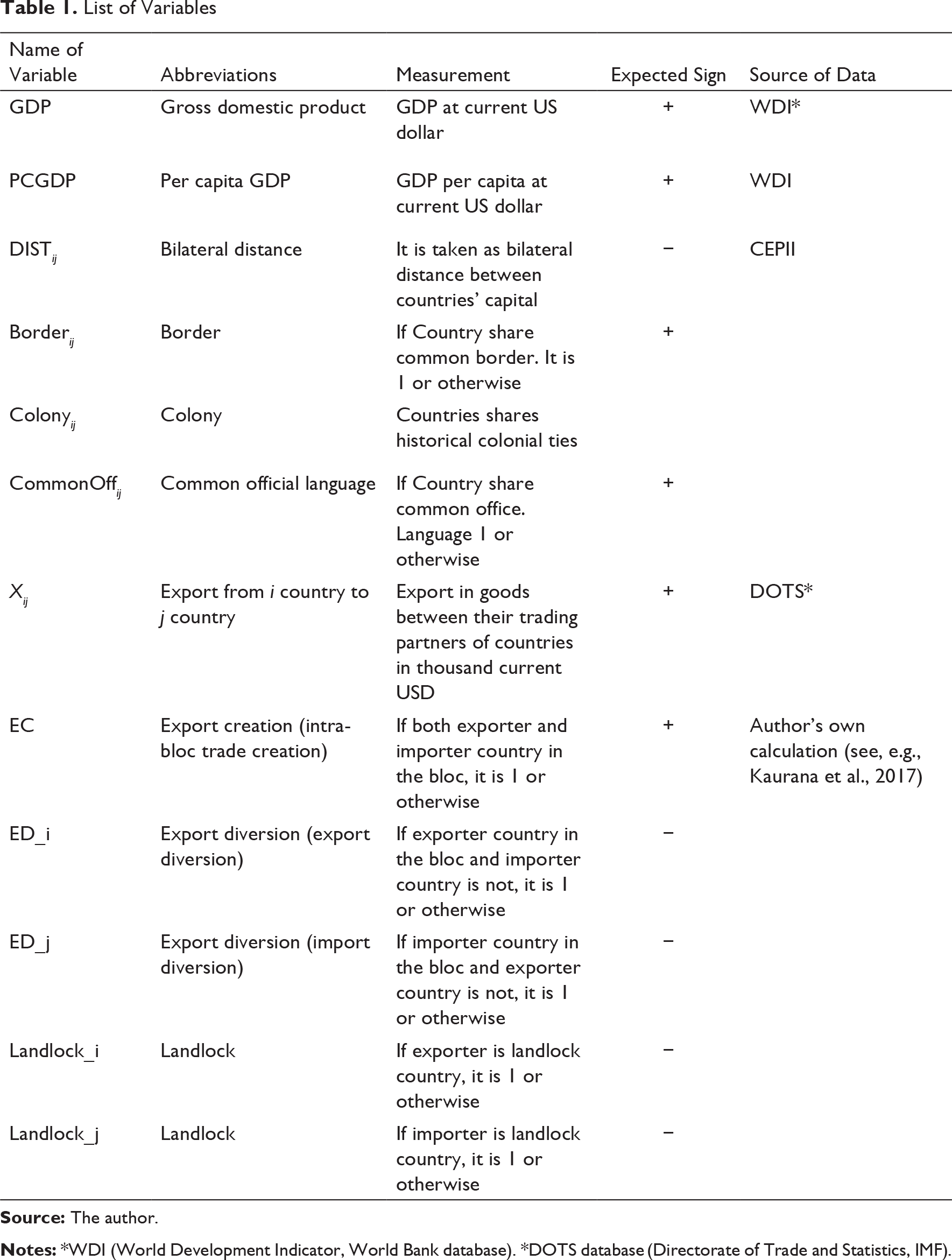
List of Variables
Formulation of Gravity Model
Descriptive Statistics
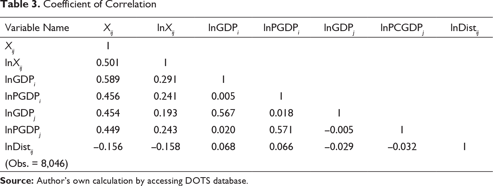
Coefficient of Correlation
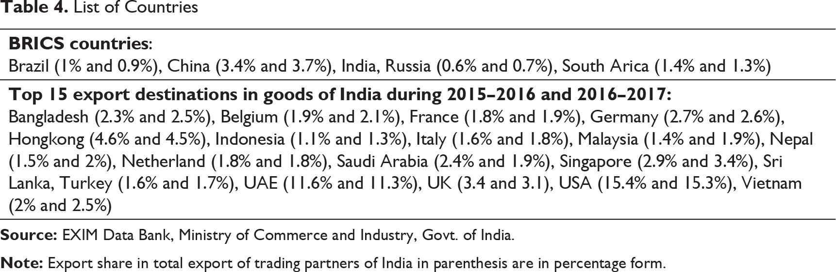
List of Countries

In general, the expected signs here are β1; β2 > 0. However, the economics of Equation (3) can lead to the interpretation of GDP as income, and when applied to agricultural goods, Engels’s Law allows for GDP in the destination country to have a negative influence on demand for imports. Hence, it might be possible that β2 < 0.

Furthermore, if we write in econometric form, we can write Xi is trade or export (import), Yin is a combination of n number of macro-variables, for example, per capita GDP. Similarly, Zjm is a combination of m number of indicators of trade cost, which may impede (foster) the trade. In addition, μi is the random term or stochastic term; βn and γm are coefficients of the respective indicators, either macro-variable or trade cost variables. The analysis of gravity model is traditionally estimated by using cross-sectional data. But it is not able to control for unobserved and individual heterogeneity (importer and exporter fixed effects), bilateral effect, heteroscedasticity, measurement error, etc. Therefore, it is argued by several economists that panel data framework is most appropriate. Furthermore, MRTs should be included in the model, use unidirectional flow rather than total or average or aggregate trade flow and do not deflate trade flows. This also eliminates time-invariant variable estimation problems (see Anderson & van Wincoop, 2003; Baier & Bergstrand, 2007; Baldwin & Taglioni, 2006; Head & Mayer, 2013; Silva & Tenreyro, 2006).
Econometric Specification of Model
Baseline Model
To capture Viner’s (1950) conceptual framework, three dummy variables (Djh) are introduced to check the effect of TC (TD) as described in Yang and Martinez-Zarzoso (2014), Kahouli and Maktouf (2015), Khurana and Nauriyal (2017). In addition, this approach is different from Viner’s (1950) approach. But it gives the same meaning as TC (TD). This is an extension of Viner’s (1950) approach in empirical analysis. The details of variables and measurement are described in Table 1. The non-linear equation seems to be
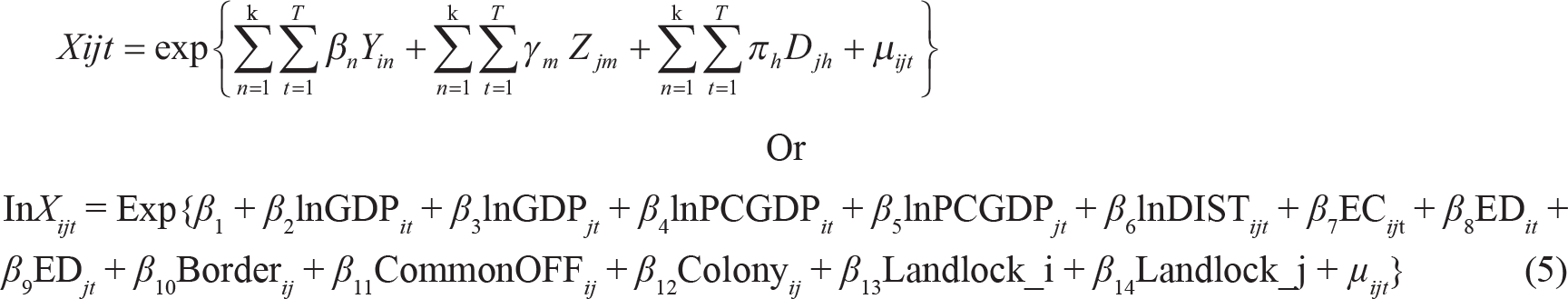
where Xijt is export of i country to j partner trading country, GDPi(j) represents the positive relationship with trade (export) and exporter income (GDPi) reflects production capacity of an economy, while importer income (GDPj) indicates about purchasing capacity of an economy. PCGDPi(j) shows a positive association with respect to trade. In general, per capita income refers to the level of development of countries (infrastructure, endowments). Moreover, higher the exporter PCGDP, more are willing to export the product. Conversely, higher the importer PCGDP reveals more ability to demand. Thus, higher per capita leads to more trade, for example, Head and Mayer (2014) and Frankel et al. (1997). Furthermore, trade cost proxy by the distance between the centres of countries. It reflects a negative relationship between trade and distance. There are other variables which affect trade, such as common official language (CommonOff), countries sharing a common border (Border) and countries having historical ties like colonial relationship (Colony). However, landlockedness of a country hinders the trade of countries; landlocked country suffers from higher trade cost. Thus, their trade cost becomes an obstacle to trade.
The year 2009 is taken, as formal annual summit began in 2009. In the case of South Africa, the dummy is calculated as equal to 1 from 2010 onwards. The ECij. refers to trade creation or intra-bloc trade effect as a result of the formation of BRICS economic bloc. A positive statistically significant coefficient sign states that trade is higher than normal levels among member nations, while a negative coefficient would reveal intra-block export diversion (Coulibaly, 2004). EDi represents TD with respect to ‘institutions’ exporting activities’. A negative and statistically significant coefficient shows that members prefer member countries to non-member countries with respect to exporting, and a positive coefficient indicates a rise in export activities from BRICS member countries to a non-member country. This is referred to as ‘export TD’ developed by Endoh (1999). EDj is an indicator of trade diversion in the import structure of the countries and referred to as ‘import TD’. A negative and statically significant coefficient states that members have diverted their importing activities from non-members to member nations. On the contrary, a positive coefficient shows that there is a growth of imports from non-members over the members (Endoh, 1999). The regional dummies permit separating the effect of the bloc, which corresponds to deviations from normal levels of trade for the sample, as predicted by the basic explanatory variables.
Equation (5) is a log transformation of the time-varying variable in the model like the pooled OLS estimated. The model does not capture the country effect and time effects. However, it has some caveats because it includes only the non-zero export values, as we know the log of zero is undetermined. To overcome this problem, we used a non-linear estimation model like the Poisson–Pseudo Maximum Likelihood (PPML) model as suggested by Silva and Tenreyro (2006). Equation (6) is estimated with time effects. This takes care of macroeconomic effects, for example, economic recessions or booms to the international flows and time trend in trade (Yang & Martinez-Zarzoso, 2014).

The next model, Equation (7), takes account of the importer- and exporter-specific fixed effects along with time effects; it captures the unobserved country-specific variables such as infrastructure and factor endowments. This also controls MRTs as suggested by Anderson and van Wincoop (2003).

In Equation (8) controls time and bilateral fixed effects. This is considered as the best one, as suggested by Baldwin and Taglioni (2006). Time effects control for macroeconomic shocks, and bilateral fixed effects control for endogeneity coming from unobserved heterogeneity between their trading partners along with all the unobserved dyad factors that do not vary with time as well as the estimable constant variables such as distance between economic centres of countries, colonial relations, common border or language (Baier & Bergstrand, 2007; Baldwin & Taglioni, 2006; Shepherd, 2013).

Finally, heteroscedasticity robust regression specification error test (RESET) is tested to check functional misspecification of each of the models. A null hypothesis, assuming that there is no misspecification, is not rejected, while rejection of a null hypothesis infers that the model has a misspecification problem.
Analysis and Empirical Results
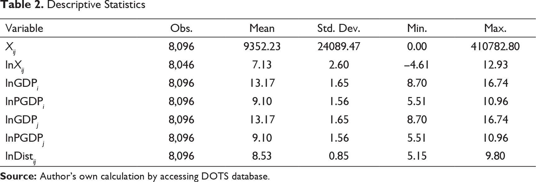
The following results are shown intabular form. Table 2 describes descriptive statistics of the study variables. Furthermore, to understand the basic relationship, the variable coefficients of correlation are calculated. The results are shown in Table 3, where we can see that GDP and per capita GDP have a positive relationship with Xij, and Xij is inversely associated with LnDistij over time (−0.158).
Results on Gravity Model of Trade
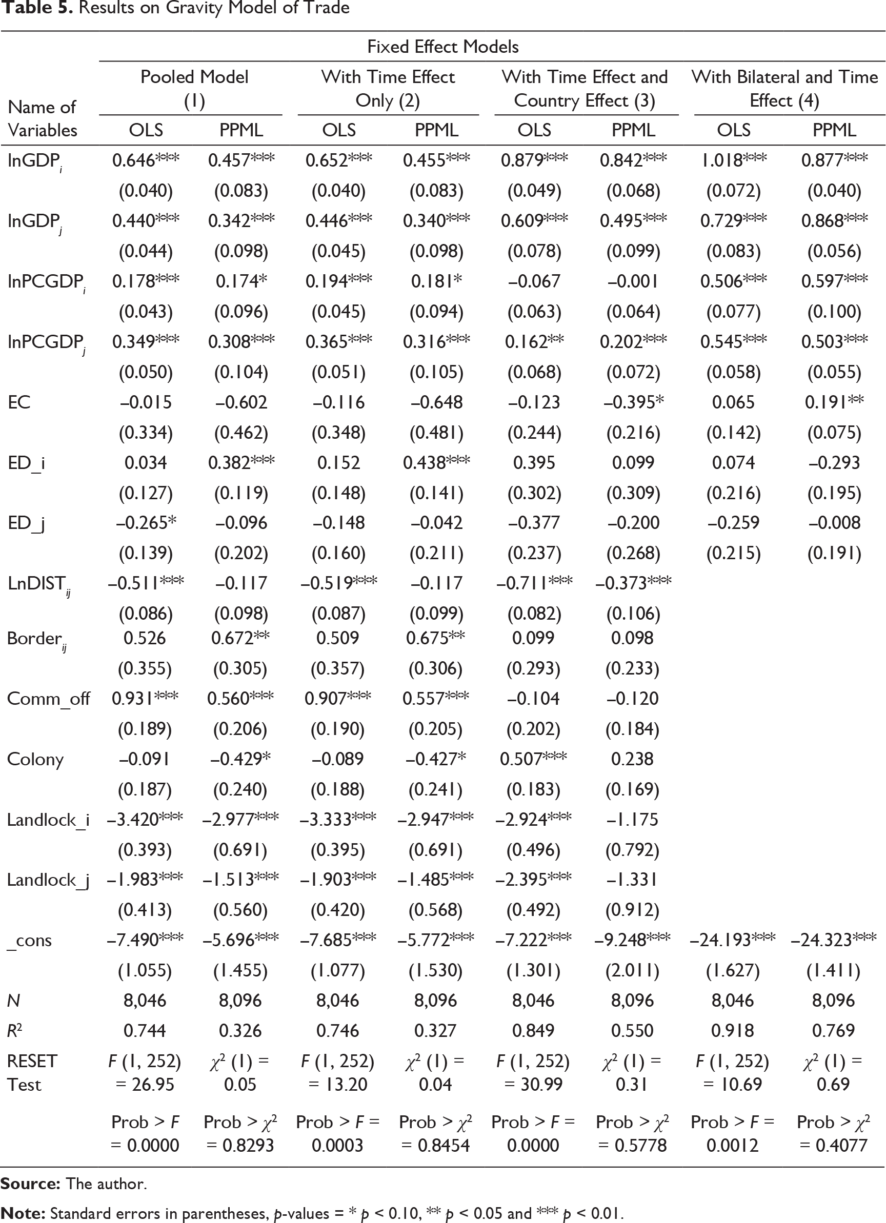
The first model describes the expected signs of traditional gravity model (see column 1). The coefficients of independent variables show exact signs of traditional gravity model, but it does not consider zero export flow. However, OLS results may not be reliable, while PPML results show slightly different results, and the RESET test passes the model. Moreover, the model shows that as the size of the economy increases, trade also increases. In addition per capita income of both exporter and importer revealed a highly significant and positive relationship with export. In contrast, as distance increases, the export also decreases. In addition, common official language and common borders show that a country’s export increases as they share a common border with each other. Interestingly, a country in colonial relationship reduces their trade with each other. In the case of TC (TD), the dummies show export diversion. This reflects the member countries’ export to non-member countries rather than member countries. This is evident in the export diversion from member to non-members countries {(exp (0.382)−1 × 100) ≈ 46.5%}, which is higher than expected from the normal level of trade. However, the landlocked problem reduces exports. The second model validates previous model estimates (see column 2). This model includes a time fixed-effect model. Of course, PPML results are more precise compared to OLS results, and the RESET test passes the model. However, the coefficient of export diversion is significant. This reflects member countries’ export to non-member countries rather than member countries. This is evidenced by the export diversion from member to non-members {(exp(0.438)−1 × 100) ≈ 55%}, which is higher than expected from a normal level of trade. However, the landlocked problem hinders trade; the magnitude is −95 per cent (−77%) likely to reduce export and import from expectation if exporter (importer) is a landlocked country. The third model includes time and country fixed-effect model. The model revealed the economic size of countries, whereas importer per capita income coefficients are significant and indicate a positive sign (see column 3). However, distance and export creation (ECij) depicted a negative sign. Moreover, a 1 per cent increase in distance is likely to reduce export by −37.3 per cent, and export creation variable shows {(exp(−0.395)−1 × 100) ≈ −100%}, which is likely to intra-bloc TD taking place above than normal level. In addition, the model passes the RESET test. Finally, the fourth model (see column 4) includes time and country bilateral fixed-effect model. Moreover, both models pass the RESET test. The model revealed the economic size, and the per capita income countries are significant and positive. Interestingly, the coefficient of export creation is significant and positive. This model is considered to be the best one. This model considers only the dyad factor. The model computed on the cost of omitting time-invariant variables like distance and common official language. This reflects member countries’ export to members’ countries. This is evident in the marginal export creation {(exp (0.191)−1 × 100) ≈ 21%}, which is higher than expected from a normal level of trade. Moreover, this model captures macroeconomic shock and unobserved heterogeneity because of trading partners. Thus, the model is free from all endogeneity problems and heterogeneity problem. This model concludes that there is marginal export creation (21%) observed in the BRICS countries since its inception.
Discussion
The results of these models revealed almost as expected. The results estimated from PPML models are more precise to estimated OLS Models. This model is often called a constant elasticity model, for example, Silva and Tenreyro (2006). Precisely, elasticity should be equal to or less than unity. The elasticity of income of exporter (importer) GDP is as expected; this is also evident in Yang and Martinez-Zarzoso (2014), Kahouli and Maktouf (2015), Khurana and Nauriyal (2017). In addition, the exporter (importer) per capita income (PCGDP) showed a significant relationship. This implies that per capita income facilitates trade and increased productivity level in exporter countries, while people in the destination market are willing to purchase more or demand more. This is also evident in Yang and Martinez-Zarzoso (2014), Kahouli and Maktouf (2015), Khurana and Nauriyal (2017). Results of trade cost like distance coefficient shows constant elasticity, and its sign is negative as expected. Conversely, cultural indicators like common official language positively affect trade. Moreover, colonial ties and common border sharing also positively affect trade. These results are as expected in line with Cheng and Wall (2005), Kristjánsdóttir (2005), Silva and Tenreyro (2006), Chi (2010), Bergeijk and Brakman (2010), Doumbe and Belinga (2015), Mishra et al. (2015), Yang and Martinez-Zarzoso (2014), Kahouli and Maktouf (2015), Khurana and Nauriyal (2017). Results are observed based on Viner’s (1950) framework trade creation. This is also observed in Yang and Martinez-Zarzoso (2014) and Kahouli and Maktouf (2015). This revealed that countries are trading more between member countries, thereby showing an increase in welfare. In a similar manner, β7 + β8 > 0 and β7 + β9 > 0 are observed as pure trade creation in terms of exports (imports) and vice versa.
Conclusion
This article tried to analyse the BRICS countries performance with respect to trade, specifically, in the case of goods export to BRICS countries. Since some countries are situated in different continents and show enthusiastic cooperation among themselves, the effectiveness of BRICS needs to be thoroughly examined. Thus, the study tried to answer whether trade in goods accelerated during post-BRICS economic bloc formation. To answer this question, this article attempted to conduct an empirical investigation of the augmented gravity model of trade for India’s direction of trade with BRICS and top merchandise export partner countries over the period 2001–2016. The results validate the traditional results of the gravity model in the context of India as well as rest of the BRICS countries. Evidence on trade creation has also been observed. However, trade cost is the biggest concern for these countries as 37 per cent of export decreases due to a 1 per cent increase in distance. Again, the common official language, contiguity or common border boosted exports. But, a landlocked country experiences reduction in export due to difficulties in accessing transport facilities, either through sea route or through roadways. Therefore, connectivity is still the biggest concern. Typically, trade creation effect contributed to Russia and China, whereas Brazil, India and South Africa gained lesser advantage. Furthermore, these kinds of forums contribute not only to boost trade but also improve cooperation among the nations, political stability, cultural exchange, and collaboration in research and development and regional development of the region. It also plays a role in shaping the global power dynamics.
Eventually, this study contributes to future research on bloc evaluation with respect to trade among the BRICS bloc. This is the first attempt to study the bloc in reference to trade bloc although it is not a trade bloc. It also gives a hint as well as guidance to future researchers to examine trade at the product level of the BRICS bloc. The findings suggest that BRICS countries may pursue trade agenda positively. Nevertheless, product-level analysis is required to explore additional trade benefits.
Managerial and Policy Implications
On the policy implications, the BRICS countries need to develop good transport connectivity to facilitate the export of goods. Further, to protect each national interest, there should be a mutual understanding that strengthens trade relationship, and trade talks should take place to boost trade among them. In addition, countries need constructive policy dialogues among nations. Moreover, to reduce trade cost, countries need to invest in their infrastructure facilities, logistic facilities and reduce non-tariff barriers. The BRICS countries need to diversify their export basket, which will reduce the effects of any regional and global uncertainty of the economy in the future.
Further Scope of Research
Finally, there is scope for further studies, and need to be conducted at a sectoral level. More precaution needs to be taken while assessing at a sectoral or product level. This study can also be extended to increase trade partners that might change the result, and predictions could be more accurate.
Footnotes
Acknowledgement
First of all, this article is based on a chapter of author’s PhD thesis. Second, the author would like to acknowledge the MHRD-sponsored GIAN course on ‘Current Global Economic Policies: Issues and Analysis in Indian Context’ organized by Dept. of Humanities and Social Sciences, NIT, Tiruchirappalli, in 2017 and RIS-EXIM Bank Summer School on International Trade Theory and Practices organized by RIS, New Delhi, in 2017. Third, the author is thankful to Dr Biswajit Mandal, Associate Professor, and Prof. Sarbajit Sengupta, Professor of Economics, Dept. of Economics and Politics, Visva-Bharati (A Central University) for formal and informal discussions. Fourth, financial assistance from Indian Council of Social Science (ICSSR), New Delhi, in the form of Doctoral Fellowship is gratefully acknowledged. Finally, the author is grateful to the anonymous referees of the journal for their extremely useful suggestions to improve the quality of the article. Usual disclaimers apply.
Declaration of Conflicting Interests
The author declared no potential conflicts of interest with respect to the research, authorship and/or publication of this article.
Funding
The author received no financial support for the research, authorship and/or publication of this article.