Sage Journals: Discover world-class research

Abstract

Stock price estimation and prediction have been the popular topics for ages for various market participants, including investors, traders, financial analysts and researchers. Understanding the expected direction of stock prices can provide insights into broader market trends and sentiments. Different methods have been tried to find out future predictions with the least degree of error. Autoregressive integrated moving average (ARIMA) and artificial neural networks (ANN) are two popular methods for time series forecasting, including stock price prediction. This paper attempts to forecast stock prices with more accuracy by using ARIMA and ANN tool modelling with secondary data NIFTY 50 of the National Stock Exchange from December 2005 to July 2019. Stock price prediction through ARIMA and ANN was calculated and compared. Results obtained revealed that the ANN method of forecasting stock prices has more accuracy as compared to ARIMA modelling. Future studies can be based on different sector-based data across different sectors and stock markets.

Keywords

Stock prediction neural network MATLAB ARIMA

Introduction

With the growth of the Indian economy and various reforms regarding the securities markets, stocks have become an intrinsic part of India’s economic development, and speculation of these has become an area of concern for the people. Stock price prediction for future behaviour of the stocks has become a matter of concern not only for the investors but also for the company, market experts and researchers. Stock prices have a dynamic nature so they change quickly and in such a scenario prediction of stock price becomes difficult. Increasing advancements in technology are making it easy for stock traders to predict the price of stocks so that they can sell those stocks before the prices fall, to book profits. The availability of enormous amounts of data has made it possible to use advanced systems for stock price prediction rather than to depend only upon the experience of the stock traders.

Several techniques for the prediction of stock prices have been studied in research which can be basically divided into two categories: namely, soft computing and statistical techniques. Some statistical techniques used are regression, moving average, autoregressive integrated moving average (ARIMA), exponential smoothening and generalized autoregressive conditional heteroskedasticity (GARCH) (Wang et al., 2012). These are linear models which assume that there is a linear correlation structure among the data values of time series. Since non-linear impact cannot be captured from the above models, artificial neural network models (ANN) are used to overcome the limitations of the linear models (Banerjee, 2014; Flury & Riedwyl, 1988). ANN has a set of functions which are trained on the basis of historical data to make future predictions. Results of many papers show that while comparing the different methods, ARIMA models are found to be more robust and effective than other structural models as far as forecasting for the short term is concerned (Flury & Riedwyl, 1988; Ho et al., 2002).

There are several fields such as engineering, finance, economics and business where soft computing-based ANNs are used for forecasting and are also found superior to ARIMA predictions in many research papers (Alon et al., 2001; Bagherifard et al., Khashei & Bijari, 2010; 2012; Pieleanu, 2016). Some studies have also reported that for short-run prediction ARIMA results are better and for long-run prediction, ANN results are much better (Valipour et al., 2013).

There are several features of ANN which make them more captivating for the people working in industries and research. First, the popularity of ANN is increasing because of their ability to make composite non-linear systems for the forecasting of the time-series data. Applications of ANN have been widespread these days because of their ability to learn and predict as well as of the large storage capacity in these systems to hold (Yaseen & Okasha, 2016). These are self-adaptive systems using few assumptions and universal approximators because they can approximate a function which is continuous to a chosen level of accuracy (Adebiyi et al., 2014). These systems are also found efficient in solving non-linear problems (Khashei & Bijari, 2010). This creates a contrast between the ARIMA models and ANN as the former which are known as traditional models, assume that the series used for prediction are linear in nature but in most economic data the series used for the prediction are non-linear in nature (Pieleanu, 2016). This creates a need to study the robustness of the prediction models on the data relating to the Indian economic scenario (Banerjee, 2014). This paper applies the ARIMA model and ANN for the same time-series data set to develop a contrast between the two methodologies regarding the prediction accuracy and to confirm the contradictory results reported in prior research papers, thus finding out the dominance of one model over another.

The paper in the later part is organized in the following manner. The next section discusses the work related to the search for effective prediction techniques comprising of ARIMA and ANN and related models. Section 3 discusses the research methodology used in the study. Experimental results are discussed in Section 4 followed by the conclusion in Section 5.

Literature Review

An empirical work regarding the comparison of ANN and ARIMA results in Malaysian stock markets showed the supremacy of ANN back propagation on ARIMA results. Better prediction can be made without using extensive data from the Kuala Lumpur Stock Exchange. The paper also reported some technical problems while using ANN with the making the choice of time frames and results were good towards the end of the training period in ANN which indicates ‘recency problem’ (Yao et al., 1999).

A case of Chinese stock markets where the random walk model pattern of the stock market is tested strongly supports ANN as a potentially useful device for prediction in stock markets. The paper utilizes ARIMA, GARCH and ANN models to test whether the prices in the Shanghai Stock Exchange follow a random walk. Back-propagation algorithm is used in ANN, and all three models were compared on the basis of RMSE, MAE and Theil’s U. Results of ANN were best but not risk and transaction cost adjusted so it does not necessarily mean profitable trading always with prediction with ANN only (Darrat & Zhong, 2000).

A study concerning the U.S. stock market’s aggregate retail sales value which contains a pattern of trend and seasonality (Priyadarshini, 2015) compares traditional models such as the Box–Jenkins ARIMA model, Winter exponential smoothening and multivariate regression with ANN models. The author found ANN results closest in changing economic conditions, but the application of these models requires an expert hand on the software, and the ANN results were parsimonious as reported in the paper (Alon et al., 2001). An analysis concerning the prediction of the compressor failure for a repairable system in Singapore used ARIMA and neural network models. The results revealed that both the models were good enough for forecasting in the short run, but simulation results of feed-forward neural network were inferior to ARIMA (Ho et al., 2002).

Altay (2005) compared ANN and ARIMA forecasting in the Istanbul Stock Exchange and found that ANN outperforms ARIMA in generating good trading strategies. The paper also reports that RMSE, MAE and Theil’s U, which are the accuracy statistics to forecast are the same in value as in ARIMA models, but still, the forecasted value of ANN was better. An Iranian study forecasted Spring inflow in ‘Amir Kabir’ reservoir with the help of ANN and ARIMA models. Hydro climatological data forecast gave better results with the ANN models (Mohammadi et al., 2005). Bagherifard et al. (2012) conducted research on the prediction accuracy between ANN and ARIMA models on the Tehran Stock Exchange. The outcome of the research showed that the prediction error of the neural network was less than ARIMA results. The predictions done by both the models were quite close to the real results, but ANN model results were more accurate than ARIMA approving their supremacy on the linear model. Priyadarshini (2015) while working on the Indian stock market using Sahara mutual fund’s six years of data found the ANN results of forecasting are better than the ARIMA model. Sánchez Lasheras et al. (2015) proved the predominance of ANN on ARIMA in prediction results of COMEX (new your commodity exchange). While researching Volkswagen’s future prices in Romanian markets, the primacy of ANN over ARIMA is also proved but it was reported in the paper that during the period of study, there was a dispute involved in the company which may affect the model’s prediction (Pieleanu, 2016).

Merh et al. (2010) used ARIMA, ANN and hybrid models for forecasting in Indian stock market indices. The results showed that in many instances ARIMA predictions are better than ANN results. A study conducted on Hong Kong’s Shenzhen index used ARIMA, back propagation of ANN and a hybrid model to see the prediction accuracy of the models. The authors found that the hybrid model proposed by them was giving the best prediction results (Wang et al., 2012). The Colombo Stock Exchange has high volatility as a common phenomenon. The time-series forecasting in the Sri Lankan market done by a hybrid model of the ARIMA–ANN approach gave the best results of prediction as MAPE was the least for this model (Ratnayaka et al., 2015).

Wijesinghe and Rathnayaka (2020) used traditional techniques such as simple exponential smoothing and ARIMA have been effective in forecasting the next lag of time series. However, few studies have focused on the Colombo Stock Exchange to find new predictive approaches for high-volatility stock price indexes. This article explores whether and how newly developed deep learning algorithms for the projection of time series data, such as the Back Propagation Neural Network (BPNN), are greater than traditional algorithms. The results show that deep learning algorithms like BPNN outperform traditionally based algorithms like the ARIMA model. The MAE and MSE values relative to ARIMA and BPNN suggest BPNN’s superiority to ARIMA.

Babu and Reddy (2015) while studying the best forecasting model in the Indian stock market compared the results of ARIMA, wavelet ARIMA, GARCH and hybrid model ARIMA–GARCH. It was found that the best results were derived from the hybrid model proposed by them. Khashei and Hajirahimi (2017) used the hybrid model of ARIMA-MLP and MLP–ARIMA in series and parallel combination for stock market prediction in the Hong Kong Stock Exchange found that the series combination of the above models gave better prediction results.

Ma (2020) suggested that the ARIMA model, commonly used in stock price prediction, is a linear regression model that can be used for analysis and prediction. However, it may have some deviations when facing complex non-linear practical problems. ANN, a data-driven adaptive model, is widely used in finance, commerce and engineering. It is effective in solving non-linear problems and can provide better results in terms of stock price prediction compared with traditional models. LSTM, a variant of the recurrent neural network, has a feedback connection that makes it easier to find development trends through the back propagation of current historical prices and prices. The hybrid models are only tested in the papers they are proposed, but ARIMA and ANN are standard models and are tested on various types of data in various countries. This paper aims to find out the predictive ability of standard ANN and ARIMA regarding the stock prices of the Indian stock market index. The results of the study are based on the empirical analysis of time series data of the National Stock Exchange (NSE) of India.

Methodology

The data used in this study are from the website of the NSE of India. In the analysis part MATLAB neural network software is used for the ANN model, and EViews 9 software is used for the ARIMA model.

The data used in this empirical paper are the closing price of the NIFTY 50 index from NSE of India. NIFTY 50 is the flagship index of the NSE. It keeps track of the behaviour of the largest blue-chip companies in India and covers many major sectors of the Indian economy. NIFTY 50 stocks cover almost 65% of the total of float-adjusted market capitalization of NSE. The index data consist of high price (maximum of the day), low price (minimum of the day), volume traded, open (opening price of the index) and close price (price at time of the closure of the market). The research paper utilizes the closing price of the index for the purpose of model and prediction because it is the closing price which represents the whole day-long activity of the index. The time period of the data is from December 2005 to July 2019 which makes a total of 3,379 observations. The data of the NSE index are not stationary at the level and contain the random walk pattern. Smoothening of close values of the NSE index is done by using the 90-day moving average method to eliminate noise in data. Figure 1 shows the graph of the NSE index which helps us to know that the series is not stationary and to confirm this we use the correlogram method. The moving average of the series is taken for the study.

Figure 1.

Graphical Representation of NSE Index Close Price at Level and after Differencing.

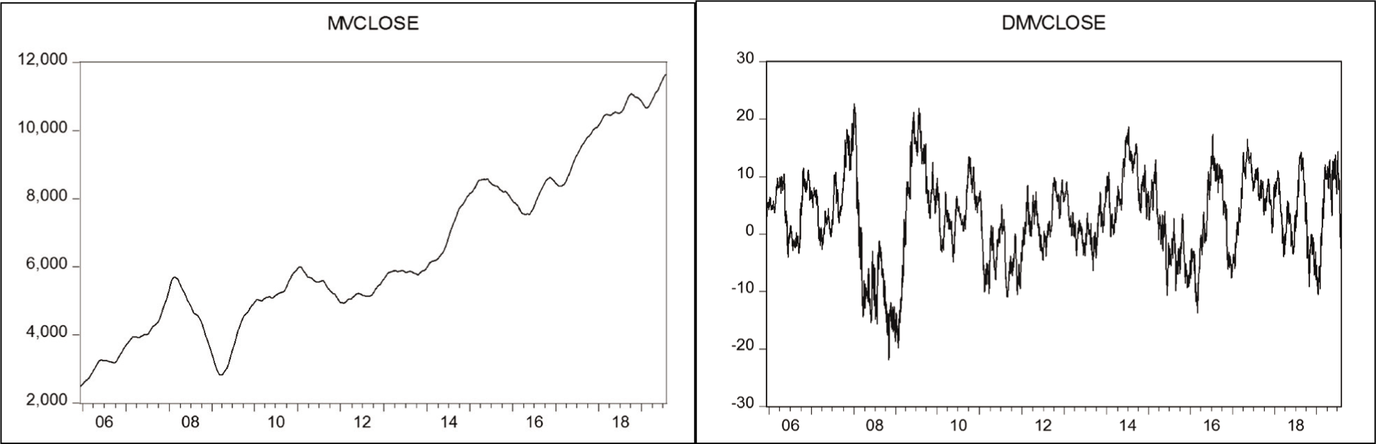
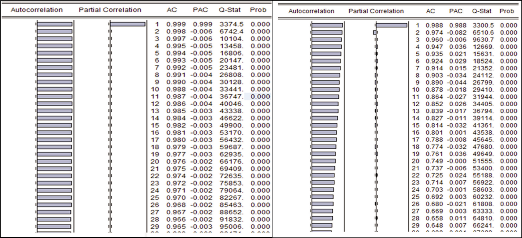
A correlogram is used to determine whether the series selected for the study is stationary or not. The autocorrelation function (ACF) of a correlogram decays rapidly from its starting point at lag 0 which that means that the series is stationary but if the ACF gradually dies down, then that means the series is non-stationary. In the case of the NSE index, the correlogram of the series dies down very slowly which proves the series to be non-stationary as can be seen in Figure 2. The series is differenced once to make it stationary and the value of the difference (d) is found by finding the number of times it is differenced.

Figure 2.

Correlogram of NSE Index Close Price at Level (Left) and after Differencing (Right).

ARIMA Model

The full form of ARIMA is the autoregressive integrated moving average. The forecasting equation contains the lag of the differenced series which are known as autoregressive terms, whereas the forecast error lags are known as moving average terms. When the time series is differenced to make it stationary it is called the integration order of the series. An ARIMA model is represented as ARIMA (p, d, q) where the number p is given to the autoregressive terms, d represents the integration order and q is given for lagged forecast error. To identify the best ARIMA model, three steps are involved as per the Box–Jenkins approach. First based on initial information a tentative model is identified. Then based on that tentative model the corresponding parameters of the model are estimated. In the last, the goodness-of-fit model is calculated. There can be several combinations for the parameters p, d, q, which are tested to find the best model on the following criterion.

Comparatively small Akaike information criterion (AIC)

Relatively small standard error of regression

Fairly high adjusted R²

There should be no significant pattern left in ACF and PACF (partial ACF) of the residuals which mean that the left residuals are white noise.

Table 1 shows the results of different ARIMA models on the NSE index.

Table 1.

Results of Different ARIMA Models on the NSE Index.

ARIMA(p, d, q)	Standard Error	Adjusted R²	AIC	SIC
(1, 0, 0)	7.99	0.99	6.999	7.004
(0, 0, 1)	1,195.160	0.74	17.013	17.018
(1, 0, 1)	5.45	0.99	6.240	6.247
(2, 0, 1)	7.99	0.99	6.999	7.004
(1, 0, 2)	4.58	0.99	5.889	5.896
(0, 0, 2)	1,195.843	0.74	17.01	17.02
(2, 0, 0)	15.94	0.99	8.38	8.38
(2, 0, 2)	8.830	0.99	7.20	7.21
(1, 1, 1)	1.148	0.97	3.117	3.124
(1, 1, 0)	7.99	0.99	6.99	7.00
(0, 1, 1)	1,195.160	0.74	17.013	17.018
(0, 1, 2)	1,195.84	0.74	17.016	17.021
(2, 1, 0)	15.94	0.99	8.38	8.38
(1, 1, 2)	4.58	0.99	5.88	5.89
(2, 1, 1)	7.99	0.99	6.99	7.00
(2, 1, 2)	8.83	0.99	7.20	7.21
(3, 1, 3)	2.08	0.92	4.311	4.319
(3, 1, 1)	1.65	0.95	3.84	3.85

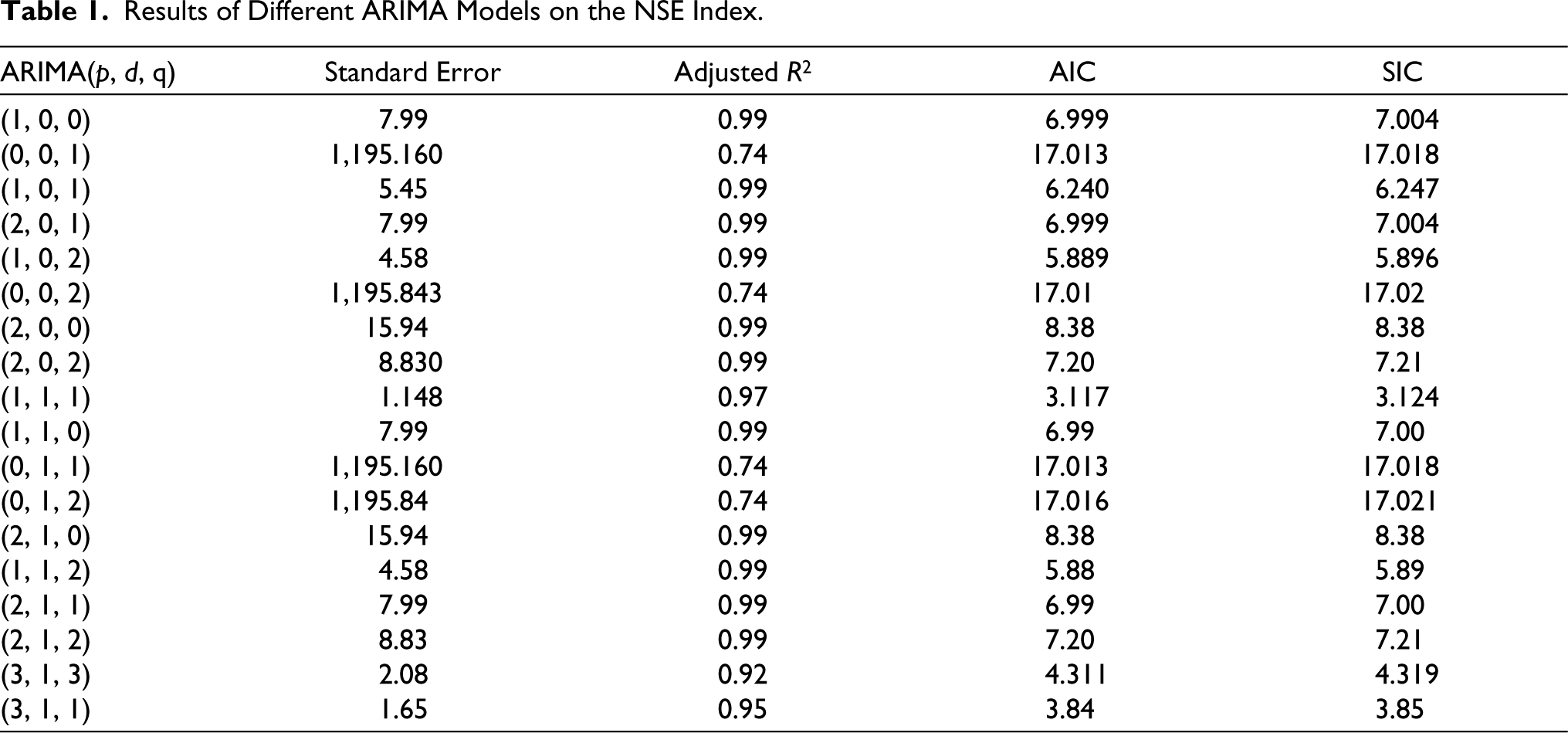
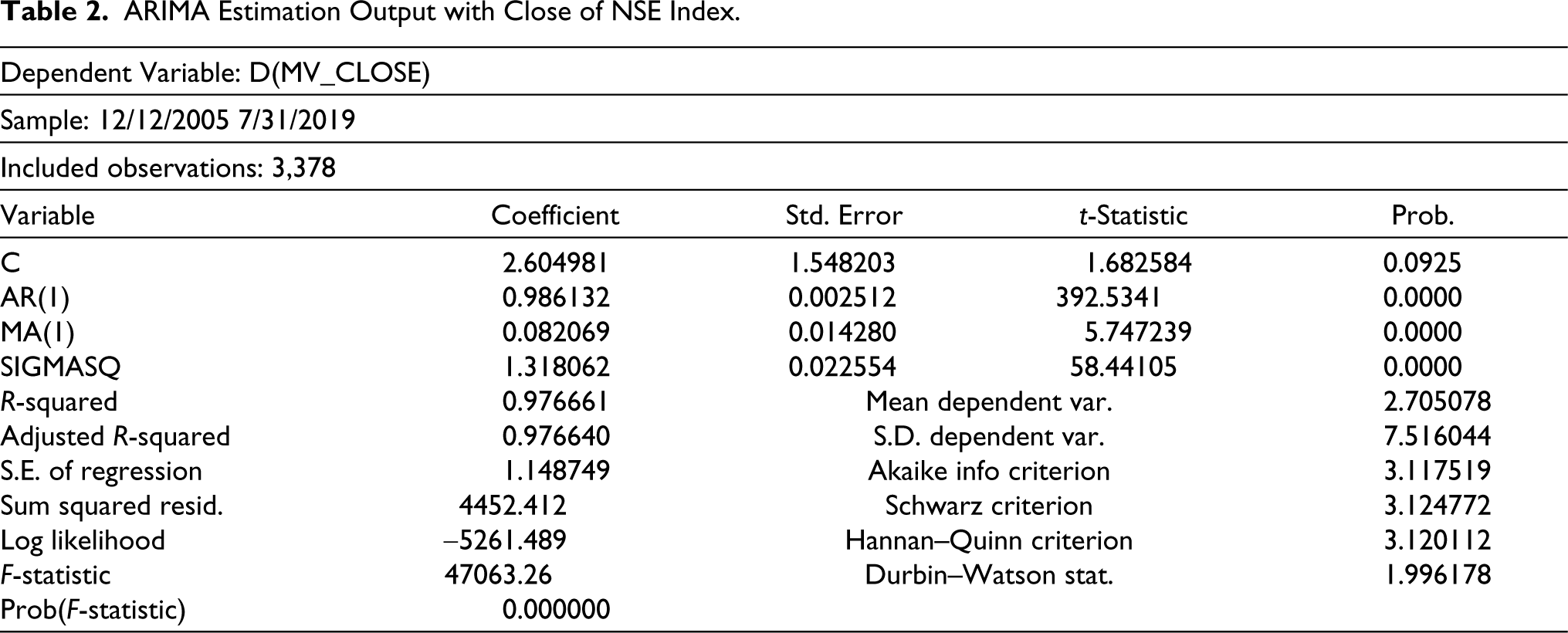
Out of the above models, ARIMA (1, 1, 1) is considered the best model as it gives the least value of standard error, AIC and BIC with the corresponding high R² as shown in Table 2. The Q statistics of the above model showed that there is no significant pattern remaining in the autocorrelation and partial ACFs of the residuals. This means that the residual of the selected model is white noise.

The ARIMA model can be expressed as:

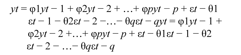
\begin{array}{l} y t = φ 1 y t - 1 + φ 2 y t - 2 + \dots + φ p y t - p + ε t - θ 1 \\ ε t - 1 - θ 2 ε t - 2 - \dots - θ q ε t - q y t = φ 1 y t - 1 + \\ φ 2 y t - 2 + \dots + φ p y t - p + ε t - θ 1 ε t - 1 - θ 2 \\ ε t - 2 - \dots - θ q ε t - q \end{array}

(1)

where yt is the model actual variable, εt is the random error, and p and q are the model parameters. The value φi (i = 1, 2…..p) and θj(j = 1, 2….q) are the order of this autoregressive model.

Table 2 shows the results of the ARIMA (1, 1, 1) model on the close price of the NSE index.

Table 2.

ARIMA Estimation Output with Close of NSE Index.

Dependent Variable: D(MV_CLOSE)
Sample: 12/12/2005 7/31/2019
Included observations: 3,378
Variable	Coefficient	Std. Error	t-Statistic	Prob.
C	2.604981	1.548203	1.682584	0.0925
AR(1)	0.986132	0.002512	392.5341	0.0000
MA(1)	0.082069	0.014280	5.747239	0.0000
SIGMASQ	1.318062	0.022554	58.44105	0.0000
R-squared	0.976661	Mean dependent var.		2.705078
Adjusted R-squared	0.976640	S.D. dependent var.		7.516044
S.E. of regression	1.148749	Akaike info criterion		3.117519
Sum squared resid.	4452.412	Schwarz criterion		3.124772
Log likelihood	-5261.489	Hannan–Quinn criterion		3.120112
F-statistic	47063.26	Durbin–Watson stat.		1.996178
Prob(F-statistic)	0.000000

The ANN Model

The term ANN, which has derived its origin from the human brain/nervous system, is developed to store various information, data and figures in a systematic form. Here in computing systems, algorithms are prepared to predict and analyse the output in advance. In the technical era, modes and methods are looked at to bring more accuracy to predictions. ANN is one such innovative method. ANN is involved in various neurons which are designed to consolidate the results depending upon the specific network design. From speech recognition to face recognition, to health care and marketing, and forecasting of future stock prices of stock, neural networks have been used in a varied set of domains. The first step towards ANNs came in 1943, when Warren McCulloch, a neurophysiologist, and a young mathematician, Walter Pitts, wrote a paper on how neurons might work (Keijsers, 2010). A neural network (Figure 3) functions when a set of data inputs are fed into the system with a special characteristic of adapting to the changing surrounding environment. This adaptability feature has been inspired from the human brain only whereby the human brain easily catches things and accordingly may relate them to the future according to the changing surroundings.

Figure 3.

A Typical Neural Network.

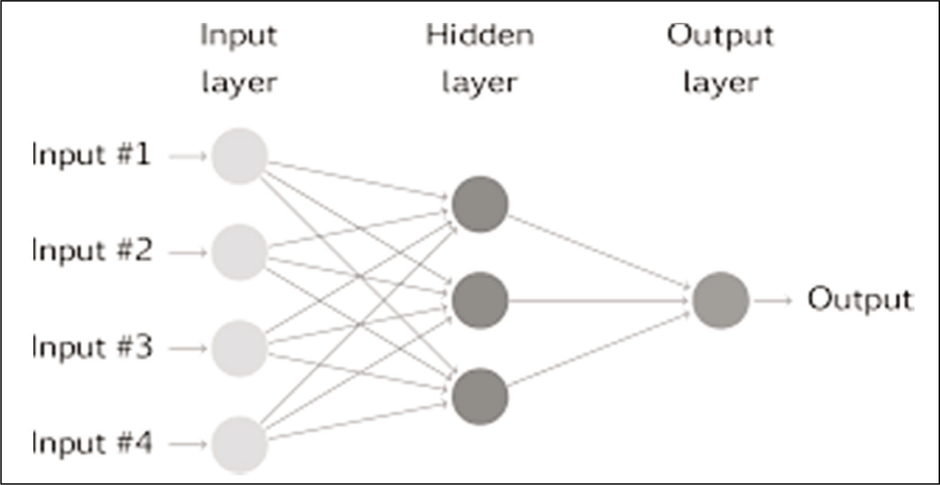
ANNs have been used widely to solve many problems due to their versatile nature (Samek & Varachha, 2013). This input layer is the main layer, and the last layer is the output layer. These data are processed through the perceptrons in order to get the desired output. Between the input and output layers, there may be additional layer(s) of units, called hidden layer(s). The connecting layers are often termed neurons.

The Neural Network Toolbox for MATLAB, developed by MathWorks, is a simulator for building ANNs. The toolbox runs under MATLAB, a linear algebra-based mathematical simulation package.

Methodology

Data Selection and Normalization

NN toolbox in MATLAB is used to predict the input data or the predicted values, as shown in the Figure 4. A time-series app is used with the closing price of the NSE to predict the future values with the help of the time-series app of NN Toolbox in MATLAB. The time-series app is useful in forecasting or prediction and hence has been taken for future prediction of stock prices. A nonlinear auto-regressive neural network (NARNN) is a recurrent neural network. It forms a discrete, non-linear and autoregressive system with endogenous inputs and can be written in the following form Ibrahim et al., 2016):

y ˆ (t) = h (y (t - 1), y (t - 2), \dots, y (t - p)) + ε (t)

Figure 4.

Neural Network Structure.

Results and Performance Evaluation

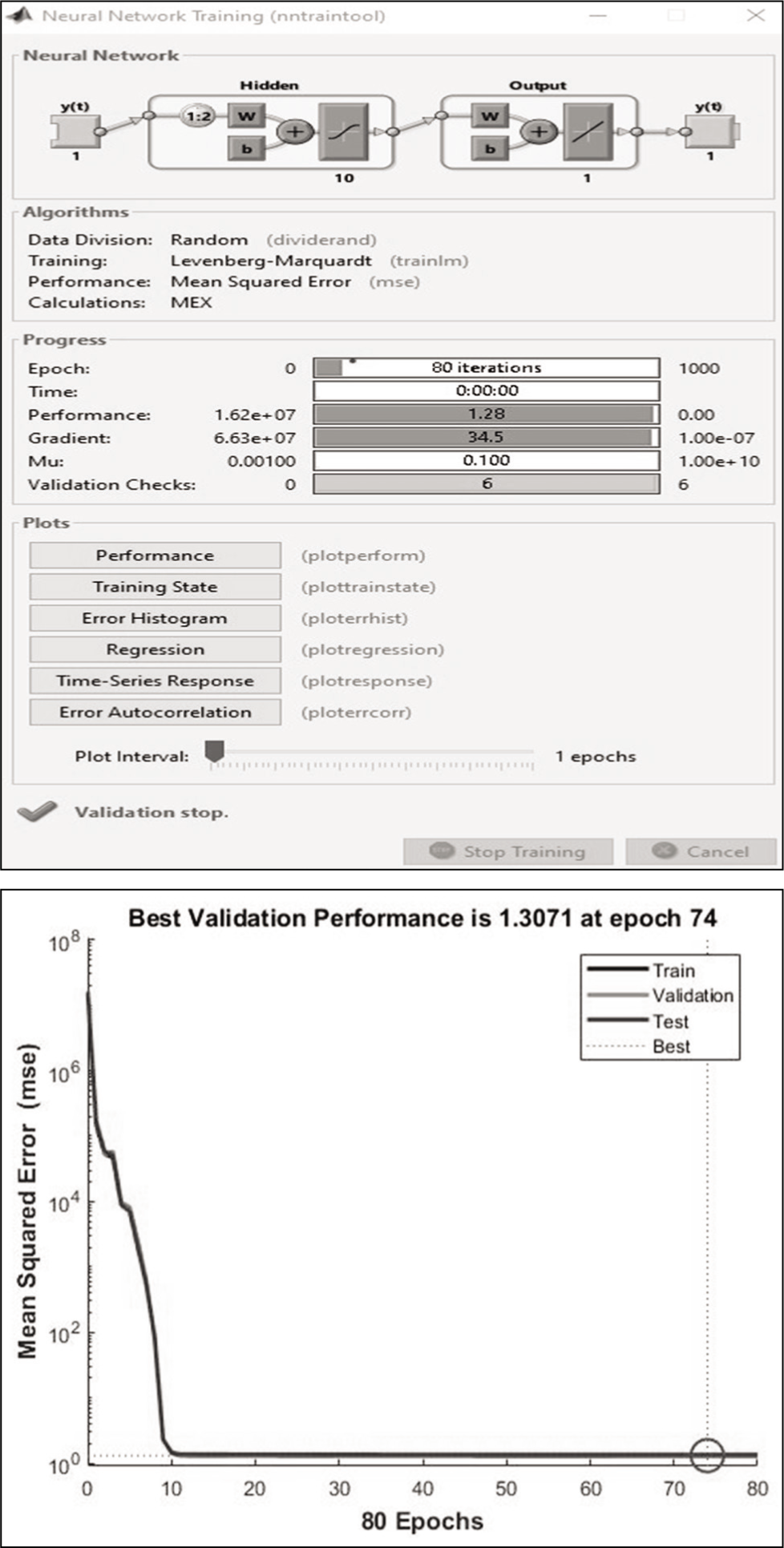
Data for this research include the closing price of the NIFTY 50 index from the NSE of India. After the network was created by MATLAB, the results were 97%, which was very encouraging for this research work. The network was trained and simulated with the Levenberg–Marquardt algorithm. Levenberg–Marquardt training is often the fastest training algorithm, as it does require more memory than other techniques and produces the output in less time. The training continued until the validation error failed to decrease for 80 iterations. Training automatically stops when generalization stops improving, as indicated by an increase in the mean square error of the validation samples. The best validation performance is equal to 01.3071 at epoch 74, as shown in the Figure 5.

Figure 5.

Graph of the Best Result Achieved in Network Training of ANN of NSE Index.

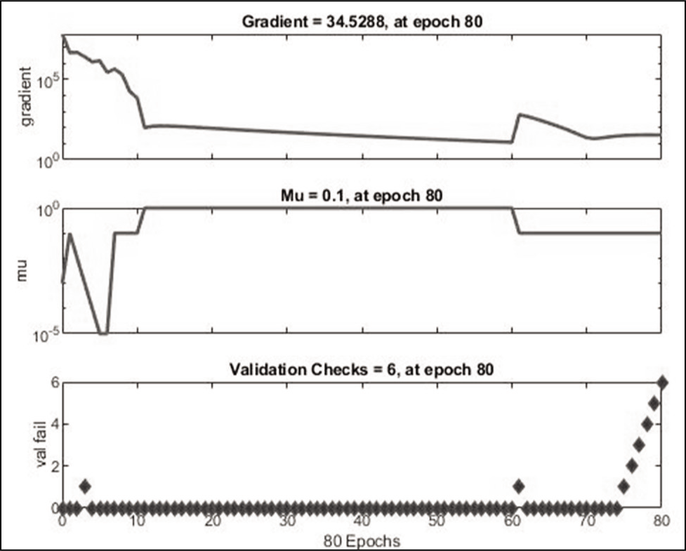
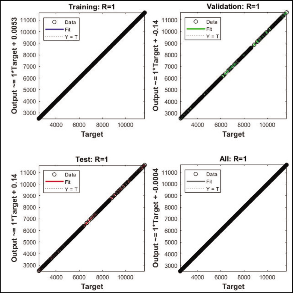
This Figures 5–7 shows that training and validation errors decrease until the highlighted epoch. It does not appear that any overfitting has occurred, because the validation error does not increase before this epoch.

Figure 6.

Regression Plots.

Figure 7.

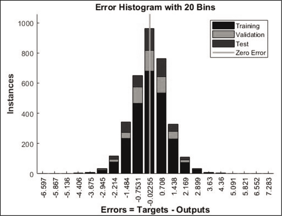
Error Histogram Plots of Predictions.

Results and Discussion

In this section, the results of the forecasting done by both ARIMA and ANN are presented.

Forecasting Results of the ARIMA Model

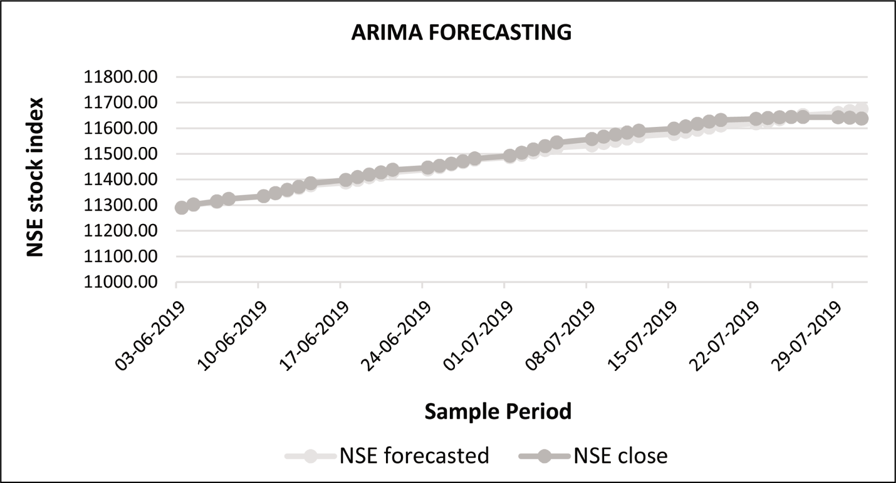
The forecasting is done after selecting the best value of both the parameters of the model, that is, the autoregressive part and the moving average part as indicated in Table 1. Models are selected on the basis of the least AIC and BIC values and high R² as shown in Table 2. Hence, the model ARIMA (1, 1, 1) came out to be the best model upon the above criterion. The forecasted and actual values of the best-fit model are presented in Table 4. The forecasting performance of the selected ARIMA model can be seen in Figure 4. To calculate the forecast error, the following formula is used.

Figure 8.

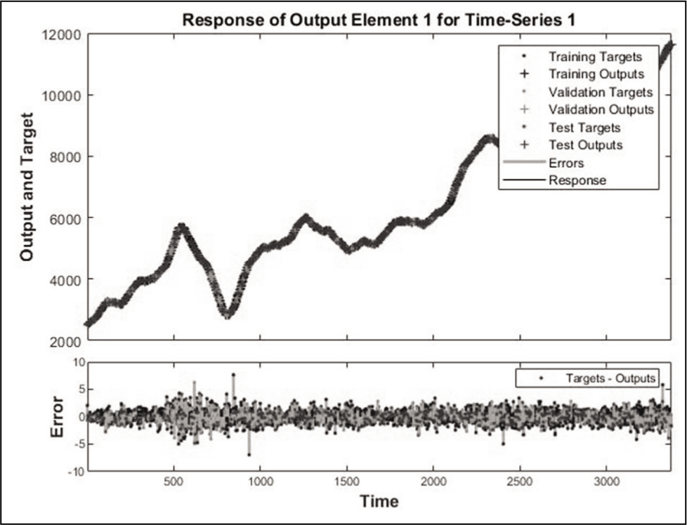
Response of Output with Reference to Time.

Table 3.

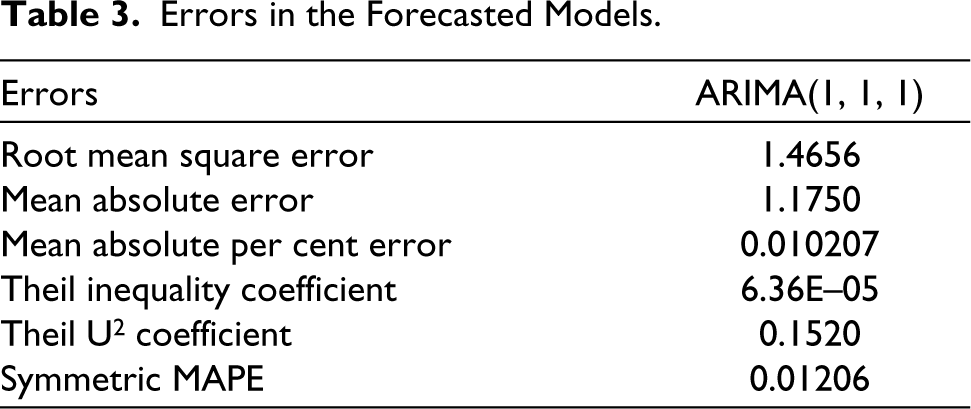
Errors in the Forecasted Models.

Errors	ARIMA(1, 1, 1)
Root mean square error	1.4656
Mean absolute error	1.1750
Mean absolute per cent error	0.010207
Theil inequality coefficient	6.36E–05
Theil U² coefficient	0.1520
Symmetric MAPE	0.01206

Table 4.

Forecasting Results of the ARIMA (1, 1, 1) Model for the NSE.

Date	NSE Forecasted	NSE Close	Forecast Error
03-06-2019	11289.65	11289.52	1.09812E–05
04-06-2019	11301.00	11302.53	-0.000135174
06-06-2019	11312.23	11314.78	-0.000224632
07-06-2019	11323.36	11324.47	-9.82051E–05
10-06-2019	11334.36	11334.88	-4.5978E–05
11-06-2019	11345.26	11346.88	-0.000142476
12-06-2019	11356.04	11359.14	-0.000272267
13-06-2019	11366.72	11371.51	-0.000420853
14-06-2019	11377.29	11385.27	-0.000700901
17-06-2019	11387.75	11398.14	-0.00091115
18-06-2019	11398.11	11409.35	-0.000985035
19-06-2019	11408.37	11418.81	-0.000914164
20-06-2019	11418.53	11427.58	-0.000792
21-06-2019	11428.58	11437.68	-0.000795625
24-06-2019	11438.54	11446.36	-0.000683403
25-06-2019	11448.40	11453.36	-0.000433573
26-06-2019	11458.16	11461.35	-0.000278561
27-06-2019	11467.83	11471.28	-0.000301467
28-06-2019	11477.40	11481.75	-0.000379163
01-07-2019	11486.88	11492.28	-0.000469231
02-07-2019	11496.27	11504.05	-0.00067635
03-07-2019	11505.58	11516.85	-0.000978824
04-07-2019	11514.79	11529.95	-0.001315047
05-07-2019	11523.92	11544.30	-0.001765878
08-07-2019	11532.96	11557.56	-0.002129115
09-07-2019	11541.91	11566.61	-0.002135273
10-07-2019	11550.78	11575.03	-0.002094562
11-07-2019	11559.57	11582.80	-0.002005369
12-07-2019	11568.28	11590.52	-0.001919112
15-07-2019	11576.90	11598.40	-0.001853515
16-07-2019	11585.45	11606.99	-0.00185579
17-07-2019	11593.92	11616.55	-0.00194826
18-07-2019	11602.31	11625.61	-0.002003723
19-07-2019	11610.63	11632.31	-0.001863368
22-07-2019	11618.87	11636.33	-0.001500345
23-07-2019	11627.04	11639.50	-0.001070136
24-07-2019	11635.13	11642.75	-0.000653644
25-07-2019	11643.16	11643.88	-6.20299E–05
26-07-2019	11651.11	11643.34	0.00066719
29-07-2019	11658.99	11642.71	0.001398355
30-07-2019	11666.80	11641.02	0.002215098
31-07-2019	11674.55	11637.26	37.28

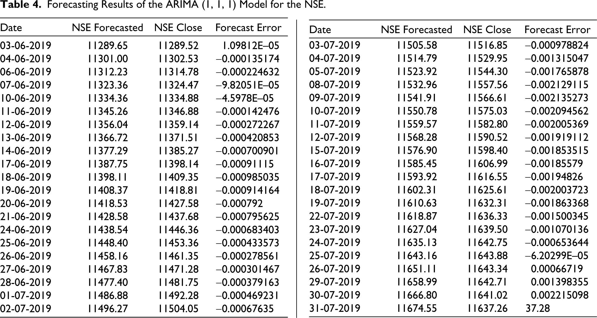
Forecast error = (actual - predicted)/actual.

Tables 3 and 4 shows that actual and predicted values vary by a very small ratio. RMSE is the gap between the actual variable and the forecasted variable, which is low and hence denotes that the predicted values are very close to the actual values. Both the values have the same direction which describes the level of precision as quite high which can be seen in Figure 4–9.

Figure 9.

The Graph for ARIMA Model Showing Actual Price Against the Predicted Values.

Comparison of ARIMA and ANN Model

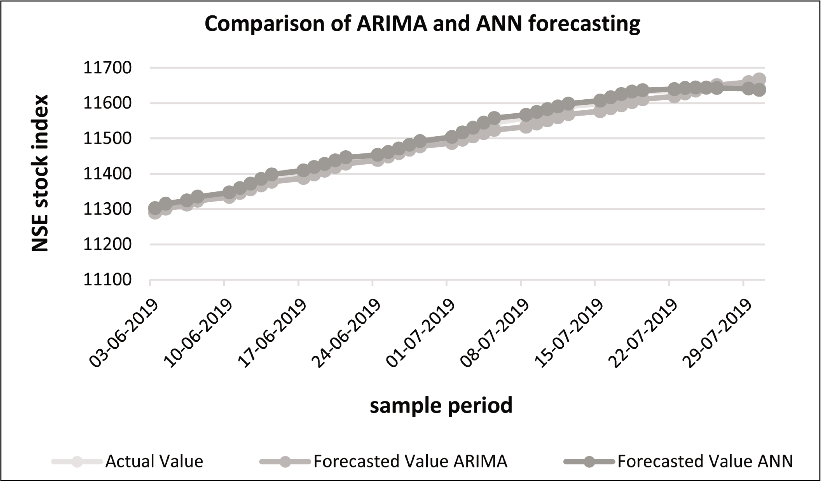
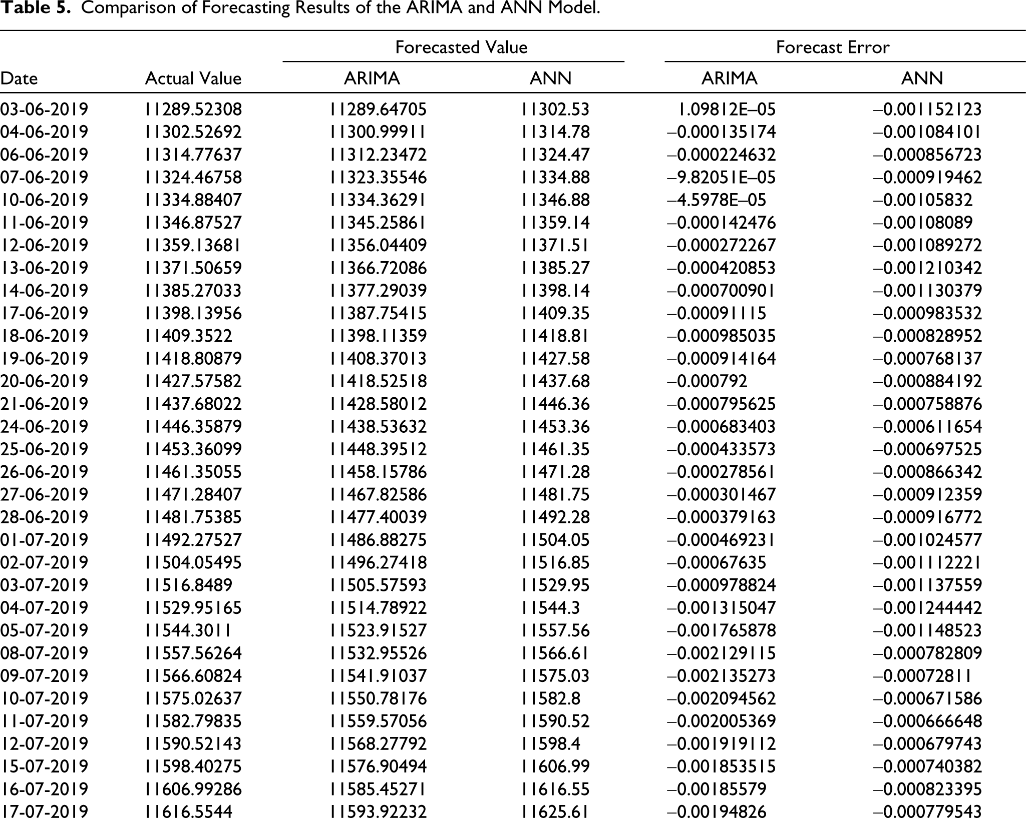
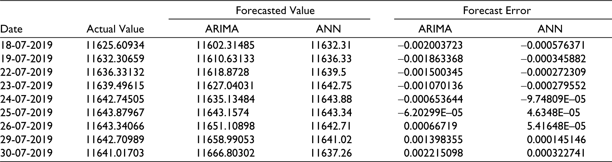
Figure 10 and Table 5 show the empirical results, and while analysing it is found that the comparison of prediction can be done by both the models. This can be clearly interpreted that these two models achieved almost near forecast performance as the forecast error resulting from them is quite low. These findings are similar to the work of Adebiyi et al. (2014). However, the prediction of ANN results is better than ARIMA results which can be seen in Figure 10. The forecasting line of the ANN model almost overlaps the actual values of the NSE index. Whereas the forecasting of the ARIMA model can be seen not exactly overlapping but with a difference. The results of ARIMA show more deviation as we reach the end of the study period. The results of the ARIMA model show a linear pattern in Figure 9; therefore, it is directional. However, the pattern followed by the ANN results in Figure 10 shows value forecasting because they almost overlap the actual values of NIFTY 50.

Figure 10.

The Graph for ARIMA and ANN Forecasting Comparison Showing Actual Price Against the Predicted Values.

Table 5.

Comparison of Forecasting Results of the ARIMA and ANN Model.

Date	Actual Value	Forecasted Value		Forecast Error
Date	Actual Value	ARIMA	ANN	ARIMA	ANN
03-06-2019	11289.52308	11289.64705	11302.53	1.09812E–05	-0.001152123
04-06-2019	11302.52692	11300.99911	11314.78	-0.000135174	-0.001084101
06-06-2019	11314.77637	11312.23472	11324.47	-0.000224632	-0.000856723
07-06-2019	11324.46758	11323.35546	11334.88	-9.82051E–05	-0.000919462
10-06-2019	11334.88407	11334.36291	11346.88	-4.5978E–05	-0.00105832
11-06-2019	11346.87527	11345.25861	11359.14	-0.000142476	-0.00108089
12-06-2019	11359.13681	11356.04409	11371.51	-0.000272267	-0.001089272
13-06-2019	11371.50659	11366.72086	11385.27	-0.000420853	-0.001210342
14-06-2019	11385.27033	11377.29039	11398.14	-0.000700901	-0.001130379
17-06-2019	11398.13956	11387.75415	11409.35	-0.00091115	-0.000983532
18-06-2019	11409.3522	11398.11359	11418.81	-0.000985035	-0.000828952
19-06-2019	11418.80879	11408.37013	11427.58	-0.000914164	-0.000768137
20-06-2019	11427.57582	11418.52518	11437.68	-0.000792	-0.000884192
21-06-2019	11437.68022	11428.58012	11446.36	-0.000795625	-0.000758876
24-06-2019	11446.35879	11438.53632	11453.36	-0.000683403	-0.000611654
25-06-2019	11453.36099	11448.39512	11461.35	-0.000433573	-0.000697525
26-06-2019	11461.35055	11458.15786	11471.28	-0.000278561	-0.000866342
27-06-2019	11471.28407	11467.82586	11481.75	-0.000301467	-0.000912359
28-06-2019	11481.75385	11477.40039	11492.28	-0.000379163	-0.000916772
01-07-2019	11492.27527	11486.88275	11504.05	-0.000469231	-0.001024577
02-07-2019	11504.05495	11496.27418	11516.85	-0.00067635	-0.001112221
03-07-2019	11516.8489	11505.57593	11529.95	-0.000978824	-0.001137559
04-07-2019	11529.95165	11514.78922	11544.3	-0.001315047	-0.001244442
05-07-2019	11544.3011	11523.91527	11557.56	-0.001765878	-0.001148523
08-07-2019	11557.56264	11532.95526	11566.61	-0.002129115	-0.000782809
09-07-2019	11566.60824	11541.91037	11575.03	-0.002135273	-0.00072811
10-07-2019	11575.02637	11550.78176	11582.8	-0.002094562	-0.000671586
11-07-2019	11582.79835	11559.57056	11590.52	-0.002005369	-0.000666648
12-07-2019	11590.52143	11568.27792	11598.4	-0.001919112	-0.000679743
15-07-2019	11598.40275	11576.90494	11606.99	-0.001853515	-0.000740382
16-07-2019	11606.99286	11585.45271	11616.55	-0.00185579	-0.000823395
17-07-2019	11616.5544	11593.92232	11625.61	-0.00194826	-0.000779543
18-07-2019	11625.60934	11602.31485	11632.31	-0.002003723	-0.000576371
19-07-2019	11632.30659	11610.63133	11636.33	-0.001863368	-0.000345882
22-07-2019	11636.33132	11618.8728	11639.5	-0.001500345	-0.000272309
23-07-2019	11639.49615	11627.04031	11642.75	-0.001070136	-0.000279552
24-07-2019	11642.74505	11635.13484	11643.88	-0.000653644	-9.74809E–05
25-07-2019	11643.87967	11643.1574	11643.34	-6.20299E–05	4.6348E–05
26-07-2019	11643.34066	11651.10898	11642.71	0.00066719	5.41648E–05
29-07-2019	11642.70989	11658.99053	11641.02	0.001398355	0.000145146
30-07-2019	11641.01703	11666.80302	11637.26	0.002215098	0.000322741

Conclusion

The study focuses on the forecasting capabilities of two models, ANN and ARIMA, for the NIFTY 50 stock index . The conventional ARIMA model which is widely used for the prediction purpose is compared with the predictive ANN model in this study. The results show that both models can achieve good forecasting results and can be used for the prediction of share prices. The forecasting values of both the forecasting models are quite close to the actual values, but the performance of the ANN model is found to be superior to the prediction done by the ARIMA model. In future studies, a hybrid model of both models can be used to find improved results from various stock indices and share prices.

In the present work, data from 2005 to 2019 were taken. Future studies can be done on a more extensive data set comprising various commodities across the stock markets.

Footnotes

Declaration of Conflicting Interests

The authors declared no potential conflicts of interest with respect to the research, authorship and/or publication of this article.

Funding

The authors received no financial support for the research, authorship and/or publication of this article.

References

Adebiyi

, & Aderemi

, & Ayo

C. K.

(2014). Comparison of ARIMA and artificial neural networks models for stock price prediction. Environmental Modelling and Software, 17(3), 219–228. 10.1016/S1364-8152(01)00077-9

Alon

, Qi

, & Sadowski

R. J.

(2001). Forecasting aggregate retail sales: A comparison of artificial neural networks and traditional methods. Journal of Retailing and Consumer Services, 8(3), 147–156. 10.1016/S0969-6989(00)00011-4

Altay

(2005). Stock market forecasting: Artificial neural network and linear regression comparison in an emerging market. Journal of Financial Management and Analysis, 18(2), 8–33.

Babu

C. N.

, & Reddy

B. E.

(2015). Selected Indian stock predictions using a hybrid ARIMA-GARCH model. 2014 International Conference on Advances in Electronics, Computers and Communications, ICAECC 2014 (October 2014). 10.1109/ICAECC.2014.7002382

Bagherifard

, Nilashi

, Ibrahim

, Janahmadi

, & Ebrahimi

(2012). Comparative study of artificial neural network and ARIMA models in predicting exchange rate. Research Journal of Applied Sciences, Engineering and Technology, 4(21), 4397–4403.

Banerjee

(2014). Forecasting of Indian stock market using time-series ARIMA model. 2014 2nd International Conference on Business and Information Management, ICBIM 2014, 131–135. 10.1109/ICBIM.2014.6970973

Darrat

A. F.

, & Zhong

(2000). On testing the random-walk hypothesis: A model-comparison approach. The Financial Review, 35(318), 105–124.

Flury

, & Riedwyl

(1988). Multivariate Statistics. Pearson. 10.1007/978-94-009-1217-5

S. L.

, Xie

, & Goh

T. N.

(2002). A comparative study of neural network and Box–Jenkins ARIMA modeling in time series prediction. Computers and Industrial Engineering, 42(2–4), 371–375. 10.1016/S0360-8352(02)00036-0

10.

Ibrahim

, Jemei

, Wimmer

, & Hissel

(2016). Nonlinear autoregressive neural network in an energy management strategy for battery/ultra-capacitor hybrid electrical vehicles. Electric Power Systems Research, 136, 262–269.

11.

Keijsers

N. L. W.

(2010). Neural networks. In Kompoliti

& Metman

L. V.

(Eds), Encycl. Mov. Disord. (pp. 257–259). Elsevier. 10.1016/B978-0-12-374105-9.00493-7

12.

Khashei

, & Bijari

(2010). An artificial neural network (p, d, q) model for time-series forecasting. Expert Systems with Applications, 37(1), 479–489. 10.1016/j.eswa.2009.05.044

13.

Khashei

, & Hajirahimi

(2017). Performance evaluation of series and parallel strategies for financial time series forecasting. Financial Innovation, 3(1). 10.1186/s40854-017-0074-9

14.

(2020). Comparison of ARIMA, ANN and LSTM for stock price prediction. E3S Web of Conferences, 218(1), 01026. 10.1051/e3sconf/202021801026

15.

Merh

, Saxena

V. P.

, & Pardasani

K. R.

(2010). A comparison between hybrid approaches of ANN and ARIMA for Indian stock trend forecasting. Business Intelligence Journal, 3(2), 23–43.

16.

Mohammadi

, Eslami

H. R.

, & Dardashti

S. H.

(2005). Comparison of regression, ARIMA and ANN models for reservoir inflow forecasting using snowmelt equivalent (a Case study of Karaj). Journal of Agricultural Science and Technology, 7(3), 17–30.

17.

Pieleanu

F. D.

(2016). Comparative study in estimating Volkswagen’s price: ARIMA versus ANN. Academy of Economic Studies Bucharest, 64(2), 98–109.

18.

Priyadarshini

(2015). A comparative analysis of prediction using artificial neural network and auto-regressive integrated moving average. ARPN Journal of Engineering and Applied Sciences, 10(7), 3078–3081.

19.

Ratnayaka

R. M. K. T.

, Seneviratne

D. M. K. N.

, Jianguo

, & Arumawadu

H. I.

(2015). A hybrid statistical approach for stock market forecasting based on artificial neural network and ARIMA time series models. 2015 International Conference on Behavioral, Economic and Socio-cultural Computing, BESC 2015 (October), 54–60. 10.1109/BESC.2015.7365958

20.

Samek

, & Varachha

(2013). Time series prediction using artificial neural networks. International Journal of Mathematical Models and Methods in Applied Sciences, 7(1), 30–46.

21.

Sánchez Lasheras

, de Cos Juez

F. J.

, Suárez Sánchez

, Krzemień

, & Riesgo

Fernández, P.

(2015). Forecasting the COMEX copper spot price by means of neural networks and ARIMA models. Resources Policy, 45, 37–43. 10.1016/j.resourpol.2015.03.004

22.

Valipour

, Banihabib

M. E.

, & Behbahani

S. M. R.

(2013). Comparison of the ARMA, ARIMA, and the autoregressive artificial neural network models in forecasting the monthly inflow of Dez dam reservoir. Journal of Hydrology, 476, 433–441. 10.1016/j.jhydrol.2012.11.017

23.

Wang

J. J.

, Wang

J. Z.

, Zhang

Z. G.

, & Guo

S. P.

(2012). Stock index forecasting based on a hybrid model. Omega, 40(6), 758–766. 10.1016/j.omega.2011.07.008

24.

Wijesinghe

G. W. R. I.

, & Rathnayaka

R. M. K. T.

(2020). Stock market price forecasting using ARIMA vs ANN: A case study from CSE. 2nd International Conference on Advancements in Computing (ICAC), Malabe, Sri Lanka, 2020, pp. 269–274. 10.1109/ICAC51239.2020.9357288

25.

Yao

, Tan

C. L.

, & Poh

H.-L.

(1999). Neural networks for technical analysis: A study on KLCI. International Journal of Theoretical and Applied Finance, 02(02), 221–241. 10.1142/s0219024999000145

26.

Yaseen

, & Okasha

M. K.

(2016). Comparison between ARIMA models and artificial neural networks in forecasting Al-Quds indices of Palestine stock exchange market. The 25th Annual International Conference on Statistics and Modeling in Human and Social Sciences; Department of Statistics; Faculty of Economics and Political Science At Cairo University. Vol. 25, 25(March 2013).

A Comparative Study of Future Stock Price Prediction Through Artificial Neural Network and ARIMA Modelling

Abstract

Keywords

Introduction

Literature Review

Methodology

Graphical Representation of NSE Index Close Price at Level and after Differencing.

Correlogram of NSE Index Close Price at Level (Left) and after Differencing (Right).

ARIMA Model

The ANN Model

A Typical Neural Network.

Methodology

Data Selection and Normalization

Neural Network Structure.

Results and Performance Evaluation

Graph of the Best Result Achieved in Network Training of ANN of NSE Index.

Regression Plots.

Error Histogram Plots of Predictions.

Results and Discussion

Forecasting Results of the ARIMA Model

Response of Output with Reference to Time.

The Graph for ARIMA Model Showing Actual Price Against the Predicted Values.

Comparison of ARIMA and ANN Model

The Graph for ARIMA and ANN Forecasting Comparison Showing Actual Price Against the Predicted Values.

Conclusion

Footnotes

Declaration of Conflicting Interests

Funding

References