Sage Journals: Discover world-class research

Abstract

Polymers play an emerging role in modern engineering applications due to their comparatively low cost, low density, and versatile manufacturing. The addition of nano-sized fillers further enhances the polymer’s properties but also induces a strong dependence on the resulting microstructure, particularly the matrix-filler interphase. Since an experimental characterization of this nano-sized interphase is extremely difficult, molecular dynamics (MD) simulations are used to study the effects at such small scales. However, MD’s high computational costs usually limit the scope of a mechanical characterization. Therefore, this study presents the methodology and tools to generate and analyze samples of an efficient generic thermoplastic model. In this first contribution, we focus on the neat polymer and introduce a versatile and numerically stable self-avoiding random walker with adjustable linearity of chain growth. Moreover, we verify our equilibration procedure by preparing samples in liquid and solid state which behave physically sound. Finally, we perform uniaxial tensile tests with a maximum strain of 10 % to evaluate the mechanical properties. In the liquid case, the polymer chains are sufficiently mobile, such that the tensile stresses fluctuate only around zero, while the solid exhibits an almost linear elastic regime followed by a nonlinear part. This contribution forms the basis for a thorough mechanical characterization of polymer nanocomposites which we will address in future studies. The methodology and tools introduced are not limited to our generic polymer, but applicable to many coarse-grained models.

Keywords

molecular dynamics coarse graining material modeling self-avoiding random walk thermoplastics

Introduction

Due to constantly growing demands on modern products, such as lightweight construction, environmental justice and cost optimization, the requirements on the materials used are likewise increasing. Polymers play an emerging role in this context since they are optimally adjustable to the application. They are versatile, cost-effective to process and offer enormous potential for use especially as nanocomposites. However, for a professional application, precise knowledge of the properties of a material and their influencing factors is essential.^1,2

In engineering applications, the focus is particularly on the mechanical properties. The characteristic data and the material behavior are determined by various standardized tests which are time-consuming and expensive. Likewise, influences of the molecular microstructure, which are crucial for the fracture behavior and the outstanding properties of nanocomposites, cannot be determined by such tests. For this reason, simulations are increasingly performed, since they are more and more attractive due to steadily increasing computing power. They offer additional analysis capabilities, such as the possibility to explore the constitution of materials at much smaller length scales. The molecular level, which is particularly important for the mechanical behavior of polymers, is studied primarily with molecular dynamics (MD).

Molecular dynamics enables the mechanical characterization of the bulk properties as shown i.a. in Refs. 3–5, 6 and 7 for thermoplastics and thermosets, respectively. Furthermore, Odegard et al.^8,9 derive continuum mechanical constitutive models directly from MD simulation with their equivalent continuum method. Additionally, MD reveals mechanisms that are hardly accessible experimentally, as, for example, the formation of an interphase region surrounding the filler particles in polymer nanocomposites.^10–12 Even novel materials, such as ionic polymer nanocomposites, can be explored with molecular dynamics which was demonstrated by Moghimikheirabadi et al.¹³. However, the high computational cost associated with MD limits large scale studies, and thus more efficient models are desirable.

This work aims to outline the steps necessary to create virtual material samples of a Kremer-Grest model^14,15 for a generic thermoplastic and to perform initial deformation simulations using a uniaxial tensile test. Different configurations of the test samples in liquid and solid form below the glass transition temperature are created and analyzed in terms of their stress-strain relation. In this first contribution, we demonstrate that the generic model at hand exhibits the characteristics of thermoplastic polymers. Hence, the introduced model is suited for future investigations, for example, on polymer nanocomposites.^16,17 The subsequent characterization of the mechanical properties and the calibration of the appropriate constitutive laws will not be the aim of the work and are discussed in a follow-up contribution.¹⁷

Methods

The mechanical investigation of virtual polymer samples requires the following four steps: Definition of the material properties, creation of virtual material samples, equilibration of the samples and the actual deformation simulation. Therefore, we present the material description of a generic, efficient thermoplastic in Subsection material description, introduce our new self-avoiding random walk algorithm in Subsection self-avoiding random walk algorithm, and describe the equilibration and deformation procedures in Subsections equilibration and deformation, respectively.

Material description

On an engineering-relevant scale, material models are usually described by continuum mechanics.^18,19 As a consequence, the consideration of atomic properties and interactions are mostly not represented. However, these constitutive laws can be further improved by incorporating crucial molecular effects based on molecular dynamics simulations. Since the computational effort for these cannot consider sufficiently large particle systems in which surface influences can be neglected, periodic boundary conditions are used. In addition, for further reduction of computational cost, repeating atomic structures are substituted by so-called superatoms in the coarse graining (CG) approach.²⁰ This reduces the degrees of freedom, but also neglects subatomic effects. In general, coarse graining is divided into bottom-up and top-down strategies.²¹ The former establishes a structural mapping based on atomistic reference simulations and thus transfers the chemical and physical characteristics to the coarse-grained scale.²⁰ Bottom-up coarse graining typically suffers limited transferability to different thermodynamic states²¹ and distorted dynamics.²² On the contrary, the coarse-grained potentials are calibrated based on experimental observations in the top-down approaches. The resulting models lack the chemical detail of bottom-up approaches but offer larger transferability and thus facilitate crucial insights into polymers’ structure-property relations.^14,21

In general, the interactions of MD systems are based on potentials between the interacting particles while the overall thermodynamic state is defined by ensembles.²³

Unit system

We employ the Lennard-Jones reduced unit system²⁴ which is commonly used for studies on generic polymer models.^25–27 Here, all quantities are given as multiples of fundamental mass m = 1, length σ = 1, energy ϵ = 1, and Boltzmann constant k_B = 1. The conformity of the quantities with the fundamental time τ is maintained via ϵ = mσ²/τ. Consequently, all quantities presented in the following are unitless but can be mapped back to, for example, SI units,²⁸ which has been shown for commodity polymers.^29,30

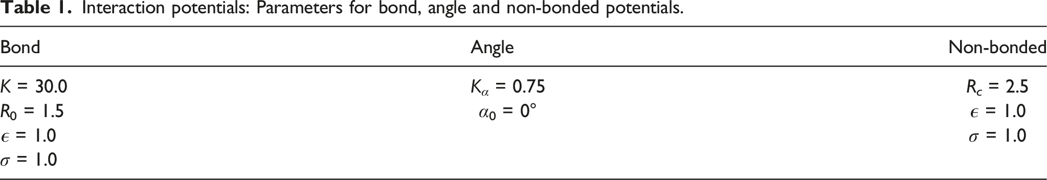
Interaction potentials

Following the top-down coarse graining strategy, we can define a generic polymer model which is, as Bocharova et al.³¹ already proved, capturing the characteristics of thermoplastic polymers. For this purpose, interactions between two non-bonded atoms as well as between two and three bonded atoms are considered. Analogously to Bocharova et al.³¹ and,³² we define the bonded interactions via the finitely extensible nonlinear elastic (FENE) potential¹⁴

E^{b} (r^{b}) = - 0.5 K R_{0}^{2} \ln [1 - {(\frac{r^{b}}{R_{0}})}^{2}] + \underset{12 / 6 Lennard - Jones (LJ) term}{\underset{⏟}{4 ϵ [{(\frac{σ}{r^{b}})}^{12} - {(\frac{σ}{r^{b}})}^{6}]}} + ϵ

(1)

with interatomic distance r^b, spring constant K, maximum bond length R₀, energy ϵ und distance σ. The angle-bending potential

E^{a} (α) = K_{α} ϵ [1 - \cos (α - α_{0})]

(2)

with angle α, equilibrium angle α₀, and the chain stiffness K_α. The bending potential is a common feature of Kremer-Grest spring bead models¹⁴ where K_α governs the flexibility of the chains from fully flexible (K_α = 0) to stiff (K_α = 12).³³ Hence, the chain stiffness has a major impact on the polymer chains’ radius of gyration and end-to-end distance.¹⁵ Furthermore, Dietz et al.³⁴ have shown the impact of K_α on the craze formation of polymer glasses. Moreover, the truncated and force-shifted Lennard-Jones (LJ) potential Eⁿ describes the interactions for particles without covalent bonds as

\begin{array}{l} E^{n} (r^{n}) & = ψ^{n} (r^{n}) - ψ^{n} (R_{c}) - [r - R_{c}] \frac{d ψ}{d r} |_{r = R_{c}} \end{array}

(3)

\begin{array}{l} ψ^{n} (r^{n}) & = 4 ϵ [{[\frac{σ}{r^{n}}]}^{12} - {[\frac{σ}{r^{n}}]}^{6}] \end{array}

with non-bonded interatomic distance rⁿ and the cutoff radius R_c. For simplicity, the generic polymer model employed in this contribution neglects a dihedral potential for interactions between four beads similar to Bocharova et al.³¹ It also comprises only one type of superatom. The necessary potential parameters are summarized in Table 1^31,32 and the potential curves are plotted in Figure 1.

Table 1.

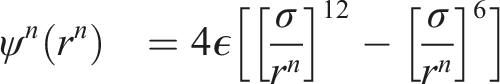
Interaction potentials: Parameters for bond, angle and non-bonded potentials.

Bond	Angle	Non-bonded
K = 30.0	K_α = 0.75	R_c = 2.5
R₀ = 1.5	α₀ = 0°	ϵ = 1.0
ϵ = 1.0		σ = 1.0
σ = 1.0

Figure 1.

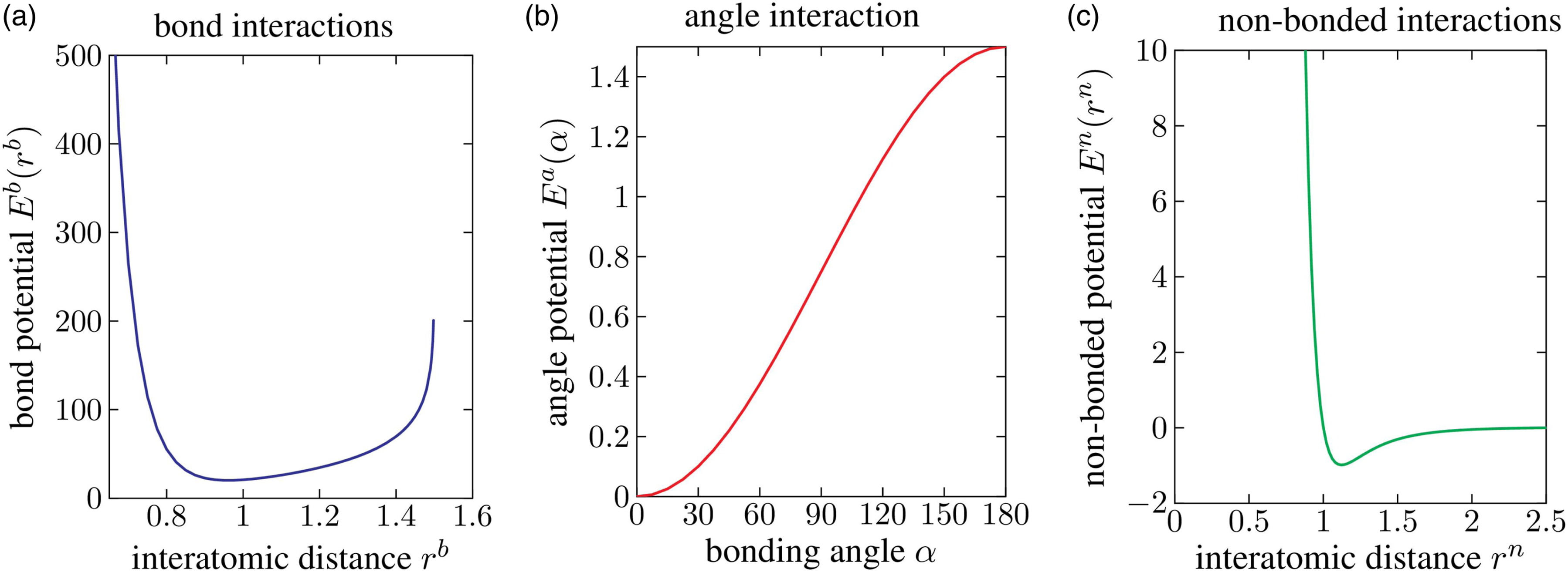
Visualization of the interaction potentials with parameters from Table 1: (a) bond, (b) angle, and (c) non-bonded potentials.

Self-avoiding random walk algorithm

After defining the particle interaction, we need to initialize their positions and connectivity to obtain the polymer samples. To this end, a self-avoiding random walk algorithm (SARW)³⁵ is introduced in the following.

The SARW’s objective is to generate a certain number of randomly arranged molecular chains with a defined number of atoms and a constant bond length. At least one atom per chain has to lie within the MD simulation box. Chains protruding from the box are taken into account via the periodic boundary conditions. The algorithm uses coarse graining and generates output files in LAMMPS’s molecular format.³² Details on the random-walk procedure are given in the supplementary information Subsection S1 and the code is publicly available via Zenodo.³⁵

To increase the SARW’s versatility, a number of parameters summarized in Table 2 can be adjusted. These are unitless and are thus easily convertible to the dimensions used for different simulations. Therefore, our SARW is not limited to our potentials and applicable for many coarse-grained thermoplastics.

Table 2.

Input parameters of self-avoiding random walk algorithm.

Variables	Explanation
bond_length	Definition of the bond distance
min_bead_distance	Definition of the minimum permissible non-bonded atomic distance (<bond_length)
num_chains	Number of molecular chains
num_beads_per_chain	Number of beads per chain
box_length	Box size for the start positions of the first atoms
min_angle	Half permissible opening angle θ of the next step in degrees
extensive_check	Extensive distance check with 26 image boxes (true or false)

Figure 2.

Validation process for a new atom within the half opening angle θ and interatomic distance greater or equal to the bond length r_b: (a) shows an invalid try for placing a new atom; (b) and (c) valid placement for a bead with a user-defined maximum allowed angle of θ = 120° for positioning new beads depicted in (c); In general, it holds for the accepted bond angle $ϕ \geq 180 ° - θ$ .

Equilibration

After a material sample is created by means of the SARW, an equilibration is necessary. Hence, the interaction potentials from the material definition (cf. Subsection material description) are assigned to the created chains and a time integration is performed for a sufficient number of time steps to reach equilibrium. This means that the resulting sample converges to a stable state and is thus ready for deformation simulations. For this purpose, the thermodynamic state, that is volume, pressure, and temperature are controlled by means of the canonical (NVT) and the isothermal-isobaric ensemble (NPT).

According to Bocharova et al.³¹, the time step size Δt is set to 0.01 and coupling times of 1.0 and 5.0 are chosen for the Nose-Hoover thermostat³⁶ and barostat,³⁷ respectively. First, an energy minimization is carried out over 2500 time steps. Second, a subsequent equilibration procedure for

9 ∙ 10^{5}

time steps ensures to reach a sufficiently equilibrated state. The applied temperature curves and ensembles used to obtain samples at T = 1.0 and T → 0 are listed in Table 3.

Table 3.

Configuration ensembles and temperature sequences in time steps at constant pressure p = 0.

Configuration	T = 1.0	T → 0.0
1. NPT holding	${7.10}^{5}$	${2.10}^{5}$
$2 . NPT cooling$	$0$	${5.10}^{5}$
$3 . NVT holding$	${2.10}^{5}$	${2.10}^{5}$
$Temperature decrement per time step$	$0$	${1.999.10}^{- 4}$

We initialize our samples at T = 1.0 since preliminary investigations have shown that the FENE bonds become numerically unstable at T > 1.0. Since this contribution is the first to evaluate the mechanical behavior of the CG model introduced in Subsection material description, only the lower (T → 0.0) and upper (T = 1.0) limit cases are considered. Note that the glass transition temperature of the present material was identified at T_g ≈ 0.41 in a subsequent study.¹⁷ Since absolute zero temperature cannot be reached due to the employed Nosé-Hoover thermostats and barostats, we apply $T = 5 \cdot 10^{- 4}$ instead. Relative pressure p is kept at 0.0 and the target temperature is T = 1.0 and T → 0.0, respectively. As stated above, we employ periodic boundary conditions and the normalized lj unit set for our three-dimensional samples. Additionally, we use the atom_style molecular and neglect bonded atoms in the evaluation of the non-bonded potentials by setting special_bonds lj to $0.0 1.0 1.0$ . Furthermore, for the neighbor list we set the extra distance beyond the cutoff to 0.3 and choose the binned style provided by LAMMPS. Additionally, the page size needs to be increased to $1.2 \cdot 10^{6}$ with $1.2 \cdot 10^{5}$ neighbors for one atom via neigh_modify to store the pairs.

Deformation

Various deformation simulations can now be carried out with the obtained samples. For a comprehensive analysis of the mechanical properties and the subsequent calibration of material laws, time-proportional, time-periodic as well as relaxation tests are required.⁴ These simulations allow for a classification into elastic, plastic, viscous, viscoelastic or viscoplastic material behavior.^38,39

However, this work aims at verifying the SARW and establishing an equilibration procedure in order to provide the basis for future investigations. Thus, we only consider the uniaxial tensile test and apply a maximum strain of 10.0 % within $1 \cdot 10^{6}$ time steps. Consequently, the strain rate

\dot{ε} (t) = \frac{ε^{m a x}}{t} = \frac{ε^{m a x}}{n Δ t}

(4)

is determined to be

1 \cdot 10^{- 5}

. All thermodynamic outputs are stored every 1000, the trajectory every

1 \cdot 10^{4}

time steps. We perform uniaxial deformation by applying a displacement in the x-direction while permitting free lateral contraction. For this purpose, the temperature is kept at a defined value via an NPT ensemble and the relative pressure for the y and z directions is fixed at

ρ = 0.0

.³¹ A more detailed discussion of the load application is given in Ref. 17 We evaluate the virial stress tensor σ,⁴⁰ whose time average corresponds to the Cauchy stress commonly used in continuum mechanics.⁴¹

Results and discussion

This section discusses the results of the equilibration procedure and the uniaxial tensile tests introduced above, which are applied to the generic polymer model used throughout this manuscript. Since we observe a tangle-like chain growth with few entanglements between multiple chains in the SARW (cf. Figure 3(a)), we examine the impact of the initial material configuration during the equilibration and uniaxial tensile test by extending the SARW in Subsection influence on the bond angles and linearity of chain growth with a partially adjustable bond angle and linearity of chain growth to perform a short parameter survey.

Figure 3.

Self-avoiding random walk algorithm with four different, examplary angle configurations: (a) θ = 120°, (b) θ = 90°, (c) θ = 50°, and (d) θ = 5°.

Influence on the bond angles and linearity of chain growth

In order to get even better control of the material generation, we impose certain constraints on the step-wise selection of new atoms without completely excluding randomness. The individual chains tend to grow like balls and thus form only few entanglements with other polymer chains, as discussed in detail in Subsection equilibration at different temperatures. To avoid this and particularly to allow for more entanglements among the polymer chains, we include an adjustable linearity of the chain growth into the code, cf. Figure 3.

In this context, we would like to remark that this also increases the numerical stability together with the flexibility of the SARW. For this purpose, the chosen option specifies an allowable angle at which the new atom may be placed. Attempts to place an atom outside the angle are not accepted and new tries are started. Furthermore, the permitted distance to other atoms has to be fulfilled, which is why the condition is automatically relaxed the more often no permissible position is found, cf. Figure 2.

The mathematical relations for implementing this procedure in the SARW can be obtained from Subsection S2 and the code is publicly available via Zenodo.³⁵ As shown in Figure 3, constraining the half opening angle θ causes the chains to exhibit different degrees of linearity in chain growth and thus different initial bond angles ϕ, depending on the angle θ.¹ In general, choosing large maximum angles θ triggers a ball-like chain growth as discussed above and it has turned out that this makes the algorithm more likely to fail. Possible remedies are to increase the simulation box size, to decrease the maximum angle θ, or a combination of both.

For the short parameter survey, we include a broad range with four different angular configurations by setting θ to 35°, 50°, 60°, and 110°, respectively.

Equilibration at different temperatures

Two different target temperatures are evaluated for the equilibration. The target temperature of T = 1.0 will create liquid material samples with low viscosity (no cooling during equilibration, cf. Table 3), while T → 0.0 (numerically applied as $T = 5 \cdot 10^{- 4}$ ) will generate solid samples with extremely suppressed dynamics (cooling during equilibration, cf. Table 3). First, the intensive quantity density is considered in Figure 4.

Figure 4.

Density during equilibration in NPT and NVT ensemble for the four samples with different initial angle constraint θ: (a) without cooling process for maintaining the target temperature T = 1.0; (b) with cooling process to target temperature T → 0.0.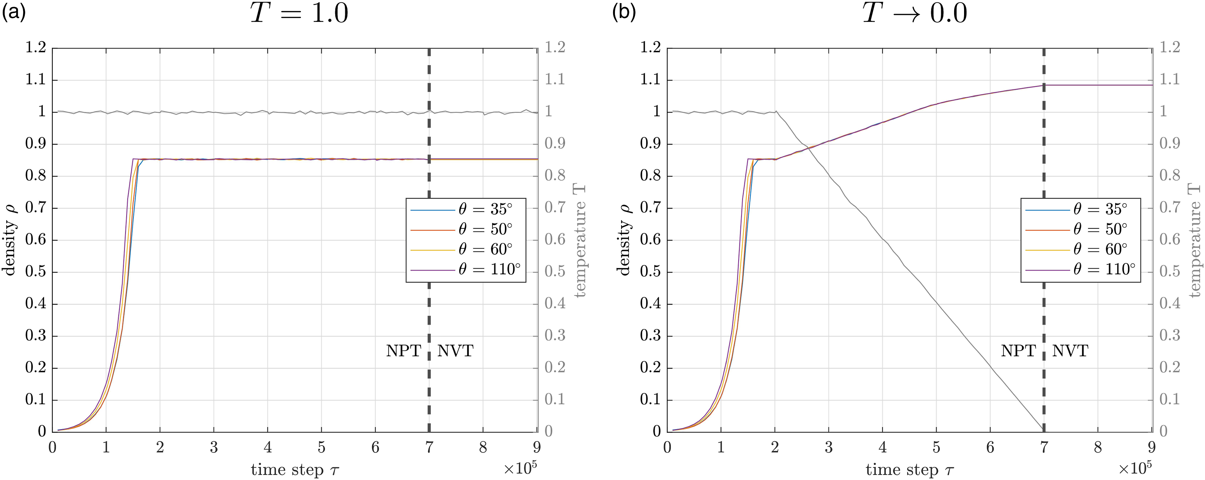

After the energy minimization, an exponential growth of density takes place over nearly $1.5 \cdot 10^{6}$ time steps until a limit of $ρ \approx 0.85$ is reached, cf. Figure 4(a). Switching to NVT ensemble at $τ = 7.0 \cdot 10^{6}$ to allow minor pressure adaptions causes no further increase in the density and confirms that the sample has reached an equilibrium. The cooling process to reach T → 0.0, cf. Figure 4(b), leads to a nearly linear increase in density until at $τ \approx 4.8 \cdot 10^{5}$ the curve flattens out and a value of $ρ \approx 1.09$ is reached. The slight density kink around $τ = 4.8 \cdot 10^{5}$ indicates a glass transition temperature of $T_{g} \approx 0.4$ coinciding with $T_{g} \approx 0.41$ reported in Ref. 17.

A difference between the four different angular configurations from the SARW is only apparent over the first $1.5 \cdot 10^{6}$ time steps. Afterwards, the difference is negligibly small.

Since the SARW generates relatively large gaps between the individual chains, the selected potentials reduce the distances between them and change the bond angles ϕ accordingly. Thermostat and barostat have been checked and are regulating the system as specified. Furthermore, the increase in density after $2.0 \cdot 10^{6}$ time steps is due to cooling of the system. A box length in each spatial direction of $l \approx 36.0$ and $l \approx 33.3$ is achieved for T = 1.0 and T → 0, respectively. Consequently, the equilibration behaves as expected.

To explain the small differences between the chains with different angular configuration, the distribution of bond angles between three atoms each is studied before and after equilibration for T → 0.0 in Figure 5. Note that most of the bond angles ϕ addressed here are $\geq 180 ° - θ$ due to the adjustable angle constraint with θ in the SARW, cf. Subsection influence on the bond angles and linearity of chain growth.

Figure 5.

Distribution of bond angles for the four samples with different initial angle constraint θ (cf. subsection 3.1): (a) before and (b) after equilibration of the samples at T → 0.0. The small sketch in (a) visualizes the increased probability that a random unconstrained atom has significantly more spherical surface available for possible positions in the range of a bond angle of 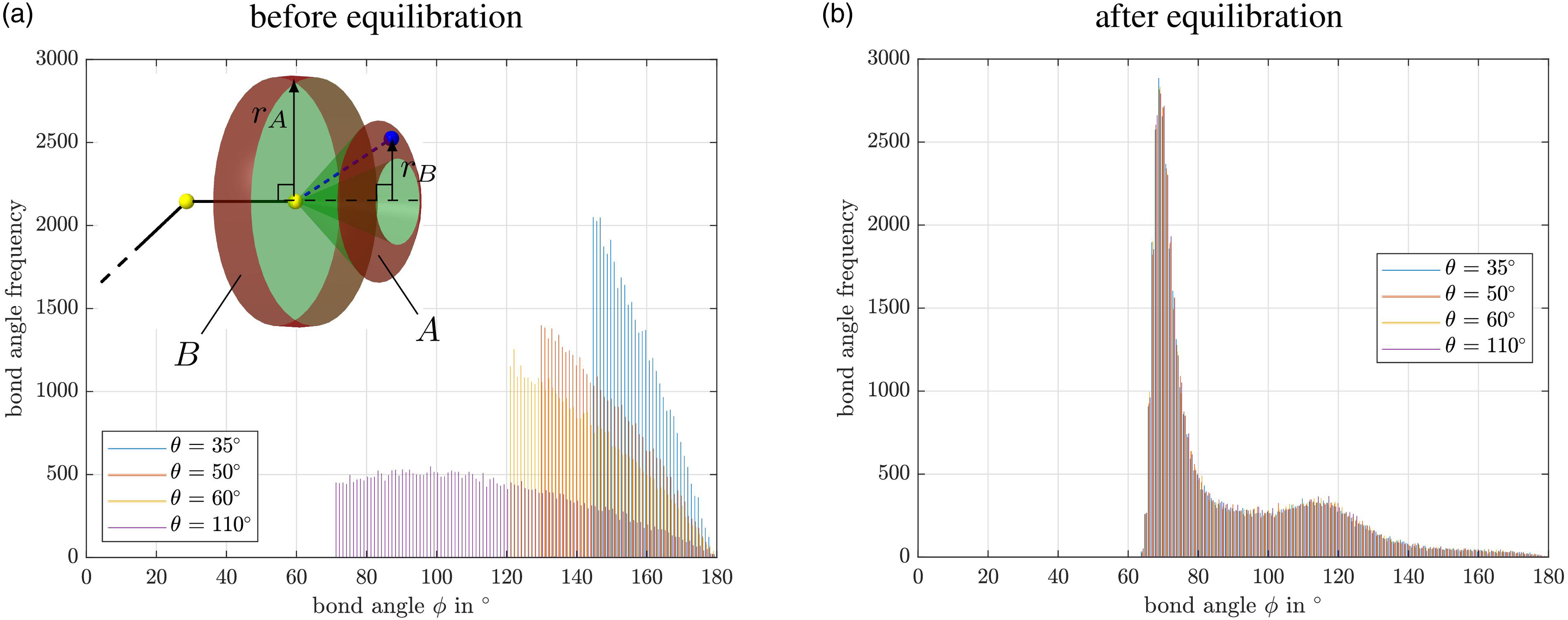$\approx 90 °$ (a sphere surface segment of area A at bond angle 155° has only $\approx 42.3 %$ of area B at 90° for each of the segment’s scattering widths of ±10°).

Before the equilibration, clear systematic differences are present in the individual samples as depicted by the histograms in Figure 5(a)). There, the frequencies of bond angles are given for different user-defined half-opening angles θ of the SARW. Due to the mentioned relation between θ and the initial bond angle ϕ, the different values of θ lead to different minimal possible bond angels for the four samples. The larger θ is chosen, the smaller the minimum bond angle ϕ gets. As expected, no angles smaller than $180 ° - θ$ occur, which demonstrates that the SARW is working properly for all four samples. In terms of frequencies, it is obvious that the maximum height of the histogram bars is larger the smaller the range of bond angles is. This is also to be expected since the number of chains as well as the number of beads per chain is the same for all systems, such that the same number of angles is to be distributed over varying ranges for the bond angles. In addition, the histogram for θ = 110° is the only one exhibiting a parabolic course with its maximum at $\approx 90 °$ .

Such a behavior is based on the increased probability that a random unconstrained atom has significantly more spherical surface available for possible positions in the range of θ ≈ 90° than at a smaller θ. For example, it is shown in Figure 5 that a sphere surface segment of area A at bond angle 155° has only $\approx 42.3 %$ of area B at 90° for each of the segment’s scattering widths of ±10°. Mathematically, this can be expressed by the circumference U = 2rπ of a circle with radius r (with r_A for area A and r_B for area B, cf. Figure 5). These radii result for θ between 0° and 180° and bond length a = 1 with the help of sine relations to $r = a \sin (θ)$ , with r_max = 1 at θ = 90°. This yields the maximum circumference U at half the opening angle θ = 90°.

After the equilibration, however, no differences between the individual material samples are visible anymore, cf. Figure 5(b). All angles are larger than 60°. At about 63°, the bond angle frequency increases very strongly until it reaches a maximum at $\approx 70 °$ . From there, the frequency drops again just as sharply and begins to flatten out to a local minimum at an angle of $\approx 100 °$ . After another slight increase, a much lower local maximum is reached at $\approx 115 °$ . Throughout the remainder of the plot, the frequency of bond angles decreases asymptotically to zero.

Markedly, Figure 5 shows that the influence of the half opening angle θ vanishes during the equilibration. After the simulation, all material samples have the same bond angles on average. It was expected that no angle smaller than 60° would be present in the materials, since the first and third atoms are so close due to the non-bonded potential that large repulsive forces are generated, preventing smaller angles. The most favorable configuration for the angles appears to be only slightly larger. There, most angles reach their equilibrium, which is a direct consequence of the defined interaction potentials. Due to the polymer’s amorphous microstructure, less favorable configurations exist as well, for example caused by entanglements. In these cases, bonded and non-bonded pair interactions are more dominant, enforcing wider angles resulting in the second local maximum at $\approx 115 °$ . Larger angles indicating almost straight chains only occur in very low numbers since stable energy states are unlikely due to extremely strong potential forces.

In conclusion, the equilibration procedure discussed here, together with the SARW introduced in this contribution, allows for a reliable and efficient creation of material samples, which can also be used for other coarse-grained materials. As demonstrated in Figure 5, the chosen parameters of the SARW do not affect the final structural properties of the material for the generic model introduced in Subsection material description. Thus, our numerically robust equilibration procedure, which is in fact insensitive to the artificially chosen chain linearity, is well suited to obtain virtual material specimens for subsequent deformation simulations.

Furthermore, the density evolutions in Figure 4 provide an estimation for the number of time steps necessary for the samples to converge. Since the equilibration covers the complete temperature range of a solid sample, it is possible to derive the necessary number of time steps at other target temperatures.

Uniaxial tension

We apply uniaxial deformation, as discussed in Subsection deformation, in x-direction and evaluate the stress response σ_xx for T = 1.0 and T → 0.0 in Figure 6(a) and (b), respectively. For the entire simulation at T = 1.0, the graphical representation shows fluctuations of the stress curve around the zero value for all material samples. The variation range is $- 0.22 ⪅ σ_{x x} ⪅ 0.22$ . Hence, no significant stresses emerge. On the contrary, for T → 0.0 an initial, linear stress increase can be seen. From a strain of ɛ_xx ≈ 2 %, the slope flattens steadily and a maximum stress of σ_xx ≈ 1.62 is reached at ɛ_xx ≈ 6 %. Up to 10 % strain, this decreases again slightly on average. The nonlinear region is characterized by strong fluctuations. Particularly evident are the deflections of the samples with θ = 50° and θ = 110° at ɛ_xx ≈ 8.7 %, whose source is not clear yet. One hypothesis is the abrupt simultaneous slipping of multiple chains.

Figure 6.

Stress-strain diagram of the uniaxial tensile test with up to 10 % strain in NPT ensemble for the four samples with different initial angle constraint θ: (a) samples with T = 1.0 fluctuate around σ_xx ≈ 0; (b) samples with T → 0.0 have a linear increase in σ_xx first before the stress-strain relation gets nonlinear and reaches a plateau.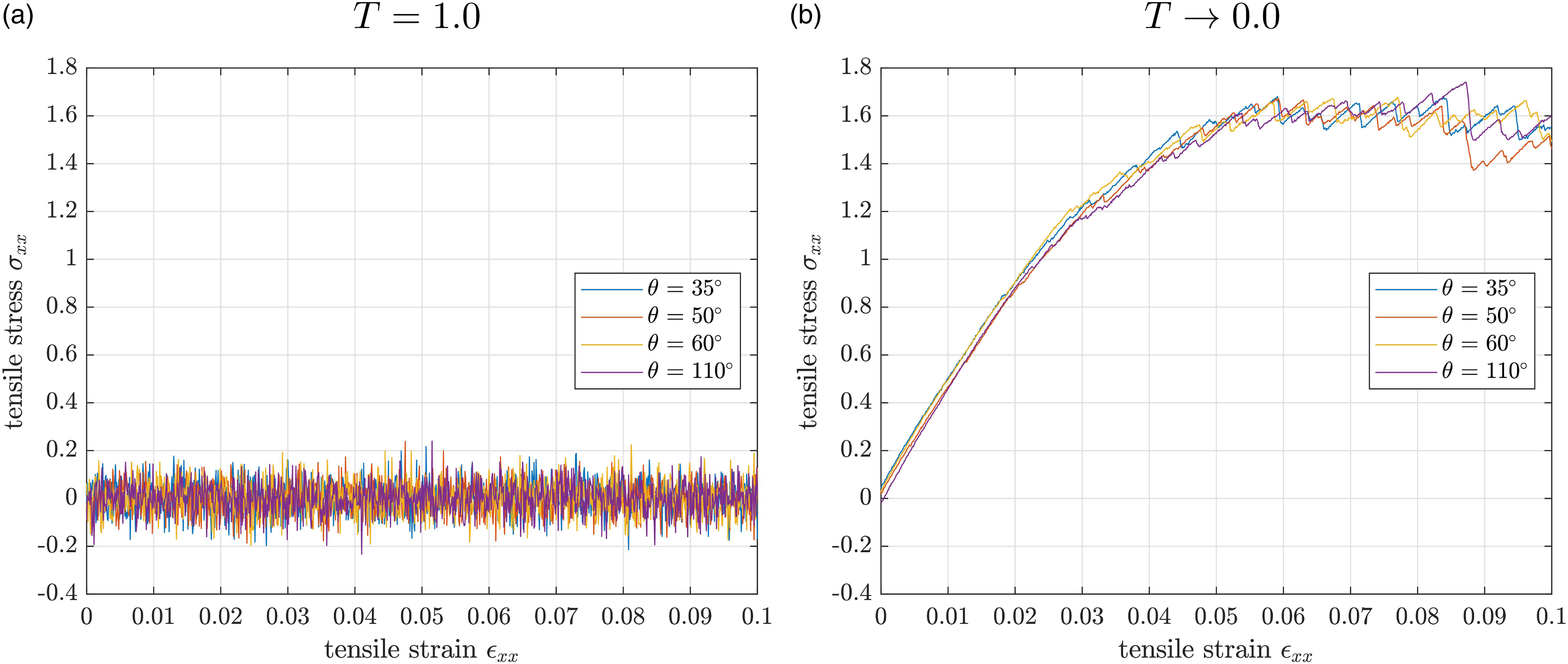

For both temperatures the stress behaves as expected: The viscosity of the liquid material samples (T = 1.0) is low enough for an instantaneous and full stress relaxation, even when 10% strain is applied. The fluctuating behavior is attributed to the temperature-induced high mobility of chains.

The samples at T → 0.0 and thus below the glass transition temperature, reveal the typical stress-strain behavior of solid polymers.⁴² In the linear elastic region, the Young’s modulus $E = Δ σ_{x x} / Δ ɛ_{x x} \approx 41.5$ is calculated as the secant up to 1 % strain. The yield stress σ_S ≈ 1.62 occurs at the yield strain ɛ_S ≈ 6 %. After that, the stress decreases, which is typical for ductile plastics.⁴² Slightly different values in the linear range are due to the random differences in the last time step of the equilibration, which form the initial configurations for the tensile test. The alternating course is likely due to the hooking of individual chains with subsequent sudden loosening along with the thermal fluctuations.

Determining Poisson’s ratio for a liquid material is not possible due to the strong fluctuations. For the solid at T → 0.0, the lateral strain in y-direction ɛ_yy is plotted over the tensile strain in x-direction ɛ_xx in Figure 7.

Figure 7.

Plot of strain in y-direction over strain in x-direction for the samples at T → 0.0.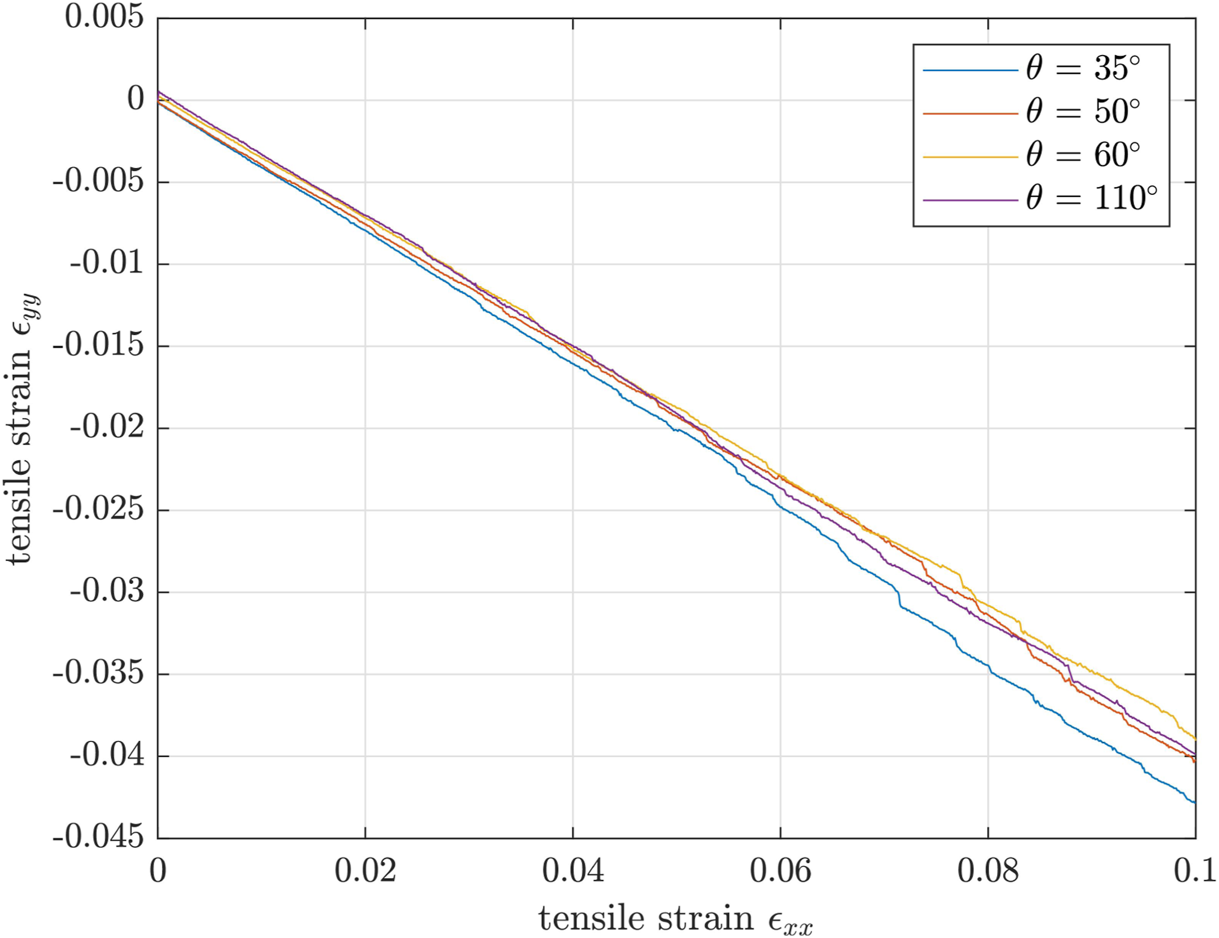

There is nearly no difference in the behavior of the individual samples and an almost completely linear curve is evident which renders an average Poisson’s ratio $ν_{x y} = - ɛ_{y y} / ɛ_{x x}$ of approximately 0.375. The sample with θ = 35° deviates at ɛ_xx ≈ 5 % from the linear path by increasing the negative gradient slightly. A subsequent contribution revealed that only minor statistical fluctuations occur,¹⁷ thus a statistical evaluation is omitted in the present study.

In addition to the conventional diagrams used to characterize mechanical behavior, the spatial arrangement of the chains is analyzed. Therefore, the movement of a single chain for a sample with T = 1.0 and T → 0 is observed during the uniaxial tensile test in Figure 8.

Figure 8.

Investigation of the spatial arrangement for an isolated chain every 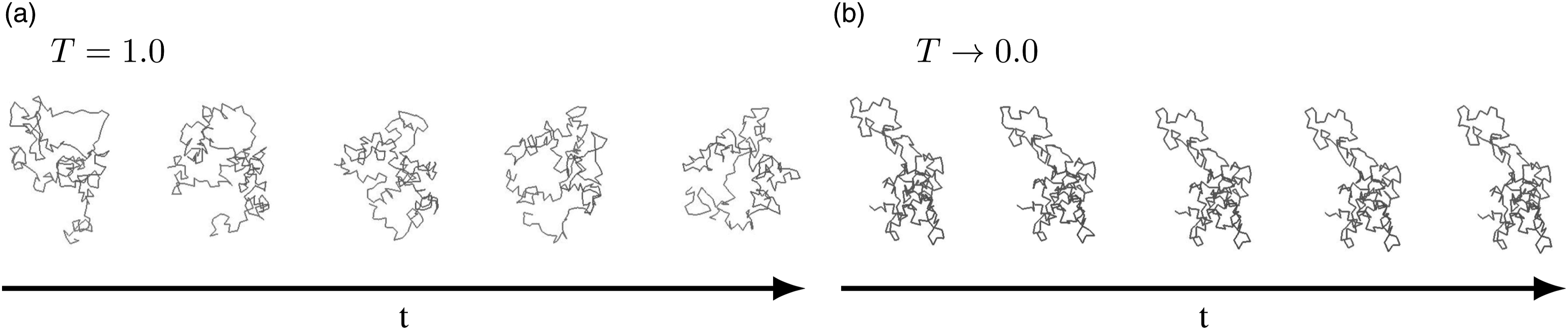$2.5 \cdot 10^{5}$ time steps: (a) major changes of spatial arrangement at T = 1.0; (b) constant chain geometry at T → 0.0.

It is clearly visible that within the considered time span in the tensile test at T = 1.0 the chain structure as well its local position change considerably. Stresses can thus be relieved due to chain mobility. In contrast, very little topological change is evident in the samples below the glass transition temperature, cf. Figure 8(b)).

The equilibration and deformation using the uniaxial tensile test at different temperatures and bond angle distributions as shown here can be used as a reference for similar systems. A complete mechanical characterization exceeds the scope of this paper and can be obtained from the follow-up contribution.¹⁷

Conclusion and outlook

In this work, the four essential steps to create virtual material samples for a generic polymer model have been thoroughly discussed. First, the properties of the material were defined using appropriate potentials. Then, an efficient, stable algorithm for the controlled creation of virtual samples with adjustable linearity of chain growth was presented. Different input parameters allow for a wide range of individual settings and thus applicability to many coarse-grained models. For the third step, the equilibration, different configurations were generated and the limited cases of T = 1.0 (liquid state) and T → 0.0 (solid state) have been studied. As a result of the SARW algorithm, different distributions of bond angles occur before equilibration, which, however, do not affect the resulting polymer systems after equilibration. In the simulations, the process for reaching an equilibrium state at the boundary temperatures of T = 1.0 (liquid state) and T → 0.0 (below glass transition temperature) was performed and analyzed. The results show that the samples behave physically sound, that is a liquid with low viscosity and comparably low density ρ ≈ 0.85 is obtained for T = 1.0, whereas a solid sample with higher density ρ ≈ 1.09 is achieved in case of T → 0.0. Furthermore, tensile tests with a maximum strain of 10 % have been performed, which also yield plausible results: In the liquid case, the polymer chains are sufficiently mobile, such that the tensile stresses fluctuate only around σ_xx = 0. In contrast, at low temperature, the stress-strain diagram exhibits an almost linear elastic part with a Young’s modulus of E ≈ 41.5, followed by a nonlinear part with a yield stress of σ_s ≈ 1.62. Furthermore, a Poisson’s ratio of 0.375 is obtained in this case.

In summary, the procedure shown here for a generic polymer model can be used as a basis for a wide variety of future studies. In this regard, the self-avoiding random walker publicly available via Zenodo³⁵ provides a practical and reliable mean to generate numerical representations of thermoplastics at coarse-grained resolution, which form the basis for our subsequent studies: As a first step, we are performing a thorough mechanical characterization of the generic polymer.¹⁷ As a second step, we incorporate nano-sized filler particles into the generic polymer to enable a mechanical analysis of polymer nanocomposites¹⁷ and their matrix-filler interphase.¹⁶

Supplemental Material

Supplemental Material - Studying the mechanical behavior of a generic thermoplastic by means of a fast coarse-grained molecular dynamics model

Supplemental Material for Studying the mechanical behavior of a generic thermoplastic by means of a fast coarse-grained molecular dynamics model by Vincent Dötschel, Sebastian Pfaller and Maximilian Ries in Journal of Polymers and Polymer Composites.

Footnotes

Acknowledgements

We thank the RRZE of FAU Erlangen-Nürnberg for providing the computational resources for this study. We would also like to acknowledge the usefulness of VMD⁴³ and its TopoTools⁴⁴ and PBCtools⁴⁵ plugins in the visualization of our systems.

Declaration of conflicting interests

The author(s) declared no potential conflicts of interest with respect to the research, authorship, and/or publication of this article.

Funding

The author(s) disclosed receipt of the following financial support for the research, authorship, and/or publication of this article: Sebastian Pfaller is funded by the Deutsche Forschungsgemeinschaft (DFG, German Research Foundation) - 396414850 (Individual Research Grant ’Identifikation von Interphaseneigenschaften in Nanokompositen’). Maximilian Ries and Sebastian Pfaller are funded by the DFG - 377472739 (Research Training Group GRK 2423 ’Fracture across Scales - FRASCAL’).

Simulation software and data

The MD calculations were performed with LAMMPS (version 29 Oct 2020),⁴⁶ while the parameter identification of the continuum mechanical models was done in Matlab.

ORCID iDs

Vincent Dötschel

Maximilian Ries

Supplemental Material

Supplemental material for this article is available online.

Note

References

Koo

. Fundamentals, properties, and applications of polymer nanocomposites. Cambridge, UK: Cambridge University Press, 2016.

Ward

Sweeney

. Mechanical properties of solid polymers. 3rd ed. Hoboken, NJ: John Wiley & Sons, 2013.

Rahimi

Iriarte-Carretero

Ghanbari

, et al. Mechanical behavior and interphase structure in a silica-polystyrene nanocomposite under uniaxial deformation. Nanotechnology 2012; 23: 305702.

Ries

Possart

Steinmann

, et al. Extensive CGMD simulations of atactic PS providing pseudo experimental data to calibrate nonlinear inelastic continuum mechanical constitutive laws. Polymers 2019; 11(11): 1824.

Ries

Steinmann

Pfaller

. Characterization of polystyrene under shear deformation using molecular dynamics. In: Developments and novel approaches in nonlinear solid body mechanics. Berlin, Germany: Springer International Publishing, 2020, pp. 219–229.

Konrad

Pfaller

Zahn

. Multi-scale modelling of plastic deformation, damage and relaxation in epoxy resins. Polymers 2022; 14: 3240.

Fan

Anastassiou

Macosko

, et al. Molecular dynamics predictions of thermomechanical properties of an epoxy thermosetting polymer. Polymer 2020; 196: 122477.

Odegard

. Equivalent-continuum modeling of nano-structured materials. Compos Sci Technol 2002; 62(14): 1869–1880.

Odegard

Clancy

Gates

. Modeling of the mechanical properties of nanoparticle/polymer composites. Polymer 2005; 46(2): 553–562.

10.

Ghanbari

Ndoro

TVM

Leroy

, et al. Interphase structure in silica-polystyrene nanocomposites: a coarse-grained molecular dynamics study. Macromolecules 2012; 45(1): 572–584.

11.

Ries

Possart

Steinmann

, et al. A coupled MD-FE methodology to characterize mechanical interphases in polymeric nanocomposites. Int J Mech Sci 2021; 204: 106564.

12.

Shandiz

Montazeri

. A novel MD-based procedure to obtain the interphase young’s modulus in nanocomposites. Comput Mater Sci 2016; 113: 104–111.

13.

Moghimikheirabadi

Karatrantos

Kröger

. Ionic polymer nanocomposites subjected to uniaxial extension: a nonequilibrium molecular dynamics study. Polymers 2021; 13(22): 4001.

14.

Kremer

Grest

. Dynamics of entangled linear polymer melts: a molecular-dynamics simulation. J Chem Phys 1990; 92(8): 5057–5086.

15.

Faller

Kolb

Müller-Plathe

. Local chain ordering in amorphous polymer melts: influence of chain stiffness. Phys Chem Chem Phys 1999; 1(9): 2071–2076.

16.

Seibert

Pfaller

Ries

. Investigation of the influence of nano-sized particles on the entanglement distribution of a generic polymer nanocomposite using molecular dynamics. Math. Mech. Solids. 2023; accepted.

17.

Ries

Seibert

Steinmann

, et al. Applying a generic and fast coarse-grained molecular dynamics model to extensively study the mechanical behavior of polymer nanocomposites. Express Polym Lett 2022; 16(12): 1304–1321.

18.

Gurtin

. An introduction to continuum mechanics. Cambridge, MA: Academic Press, 1982.

19.

Spencer

AJM

. Continuum mechanics. North Chelmsford, MA: Courier Corporation, 2004.

20.

Müller-Plathe

. Coarse-graining in polymer simulation: from the atomistic to the mesoscopic scale and back. Chem Phys Chem 2002; 3(9): 754–769.

21.

Joshi

Deshmukh

. A review of advancements in coarse-grained molecular dynamics simulations. Mol Simulat 2020; 47(10-11): 786–803.

22.

Karimi-Varzaneh

van der Vegt

NFA

Müller-Plathe

, et al. How good are coarse-grained polymer models? A comparison for atactic polystyrene. Chem Phys Chem 2012; 13(15): 3428–3439.

23.

Pfaller

. Multiscale simulation of polymers – coupling of continuum mechanics and particle-based simulation. Schriftenreihe technische mechanik Doctoral thesis, vol. 16. Erlangen, Germany: Universität Erlangen-Nürnberg, 2015.

24.

Allen

. Introduction to molecular dynamics simulation. Comput Soft Mat: From Syn Polym to Prot 2004; 23: 1–28.

25.

Dietz

Hoy

. Facile equilibration of well-entangled semiflexible bead–spring polymer melts. J Chem Phys 2022; 156(1): 014103.

26.

Nie

, et al. Molecular dynamics simulation study of the fracture properties of polymer nanocomposites filled with grafted nanoparticles. Phys Chem Chem Phys 2019; 21(21): 11320–11328.

27.

Barsky

Robbins

. Molecular dynamics study of slip at the interface between immiscible polymers. Phys Rev 2001; 63(2): 021801.

28.

Kröger

. Simple models for complex nonequilibrium fluids. Phys Rep 2004; 390(6): 453–551.

29.

Everaers

Karimi-Varzaneh

Fleck

, et al. Kremer–grest models for commodity polymer melts: linking theory, experiment, and simulation at the Kuhn scale. Macromolecules 2020; 53(6): 1901–1916.

30.

Svaneborg

Everaers

. Characteristic time and length scales in melts of kremer–grest bead–spring polymers with wormlike bending stiffness. Macromolecules 2020; 53(6): 1917–1941.

31.

Bocharova

Genix

Carrillo

JMY

, et al. Addition of short polymer chains mechanically reinforces glassy poly (2-vinylpyridine)–silica nanoparticle nanocomposites. ACS Appl Nano Mater 2020; 3(4): 3427–3438.

32.

Thompson

Aktulga

Berger

, et al. LAMMPS - a flexible simulation tool for particle-based materials modeling at the atomic, meso, and continuum scales. Comput Phys Commun 2022; 271: 108171.

33.

Hoy

Kröger

. Unified analytic expressions for the entanglement length, tube diameter, and plateau modulus of polymer melts. Phys Rev Lett 2020; 124(14): 147801.

34.

Dietz

Nan

Hoy

. Unexpected ductility in semiflexible polymer glasses with entanglement length equal to their kuhn length. Phys Rev Lett 2022; 129(12): 127801.

35.

Ries

, et al. A self-avoiding random walk algorithm (SARW) for generic thermoplastic polymers and nanocomposites. Zenodo. 2022. doi:https://doi.org/10.5281/zenodo.6245699

36.

Evans

Holian

. The nose–hoover thermostat. J Chem Phys 1985; 83(8): 4069–4074.

37.

Martyna

Tobias

Klein

. Constant pressure molecular dynamics algorithms. J Chem Phys 1994; 101(5): 4177–4189.

38.

Haupt

. Continuum mechanics and theory of materials. Berlin, Germany: Springer Science & Business Media, 2013.

39.

Pfaller

. Discrete and continuous methods for modelling and simulation of polymer materials. Habilitation thesis. Erlangen, Germany: Friedrich-Alexander-Universität Erlangen-Nürnberg, 2021.

40.

Thompson

Plimpton

Mattson

. General formulation of pressure and stress tensor for arbitrary many-body interaction potentials under periodic boundary conditions. J Chem Phys 2009; 131(15): 154107.

41.

Subramaniyan

Sun

. Continuum interpretation of virial stress in molecular simulations. Int J Solid Struct 2008; 45: 4340–4346.

42.

Sweeney

Ward

. Mechanical properties of solid polymers. Hoboken, NJ: John Wiley & Sons, 2012.

43.

Humphrey

Dalke

Schulten

. VMD – visual molecular dynamics. J Mol Graph 1996; 14: 33–38.

44.

Kohlmeyer

Vermaas

Braun

. TopoTools. Zenodo, 2020. https://doi.org/10.5281/zenodo.3845031.

45.

Henin

, et al. PBCtools (github.com/frobnitzem/pbctools). GitHub, 2022. https://github.com/frobnitzem/pbctools.

46.

Plimpton

. Fast parallel algorithms for short-range molecular dynamics. J Comput Phys 1995; 117(1): 1–19.

Supplementary Material

Please find the following supplemental material available below.

For Open Access articles published under a Creative Commons License, all supplemental material carries the same license as the article it is associated with.

For non-Open Access articles published, all supplemental material carries a non-exclusive license, and permission requests for re-use of supplemental material or any part of supplemental material shall be sent directly to the copyright owner as specified in the copyright notice associated with the article.

0.00 MB

0.56 MB