
Abstract
Tomatoes (Solanum lycopersicum L.) are a widely grown and globally traded vegetable, essential for both local consumption and international trade. However, approximately 30% of harvested tomato yields are lost due to fungal decay during postharvest handling. Timely disease identification is crucial to prevent such losses, but certain tomato varieties exhibit higher susceptibility to fungal infections than others. Additionally, there are variations in susceptibility among individual sepals, with unknown underlying causes. Traditional methods for assessing fungal presence in plants have limitations, such as sample destruction and a focus on symptom detection rather than evaluating susceptibility to fungal infection. Hence, there is a demand need for an accurate, non-destructive method capable of predicting susceptibility to fungal infection. The use of hyperspectral imaging (HSI) with chemometrics presents a pioneering approach to address this need. In this study, three tomato cultivars (‘Brioso,’ ‘Cappricia,’ and ‘Provine’) were studied. Hyperspectral images were captured on day-1 of harvest, followed by controlled fungal growth conditions. Ground truth assessments were conducted by three experts on day-3 and day-4, averaging severity scores assigned per sepal. The methodology involved extracting spectra from HSI images and calibrating and validating models using partial least squares discriminant analysis (PLSDA), aiming to optimize model parameters for accurate predictions. The models were categorized into those developed using data from a single variety (intravariety) and those utilizing data from multiple varieties combined (global models). The best-performing intravariety model was established using the Cappricia variety, achieving a balanced accuracy of 0.84. Conversely, a global model combining Cappricia and Provine varieties achieved a balanced accuracy of 0.70. Overall, the results suggest that distinguishing between more and less susceptible sepals is feasible under controlled conditions.
Keywords
Introduction
Tomato (Solanum lycopersicum L.) is a “ubiquitous vegetable.” Tomatoes are produced globally, either for domestic consumption or as a commodity for international export. The nutritional composition of this fruit includes carbohydrates, lipids and proteins. In addition, it contains vitamins, minerals, and carotenes in smaller proportions. 1
Tomato quality is divided into different aspects: commercial, organoleptic and nutritional. 2 Market quality grade considers appearance (e.g. color, form, size), firmness and shelf life, whereas health benefits rely on the nutritional value as well as on the absence of pathogenic hazards or contaminants.2–5
The portion of tomatoes that go to waste after the harvesting stage can reach 42% worldwide. 6 Around 30% of the harvested tomato produce may be lost during postharvest handling, primarily because of microbial decay caused by fungi such as Rhizopus stolonifer, Alternaria alternata, and Botrytis cinerea.7 Pathogenic fungi can infect and spread to many different parts of a tomato plant, including the stem, calyx and skin of the fruit. 8 In some countries tomatoes are sold including calyx. Fresh looking green parts of a tomato (calyx and vine) are a sign for dealing with fresh tomatoes. Older tomatoes show dehydration symptoms of the green parts. The calyx is also susceptible to infection by fungal spores. These spores may already be present on the tomato during cultivation. After harvest, under humid and poorly ventilated storage and transport conditions, these spores may germinate and grow further into visible mould on the calyx. 9 This negatively affects the value of the fruit and may lead to extra food loss and waste.9,10
The timely identification of disease has the potential to avert losses since prompt actions can be implemented to mitigate further damages (e.g. adapt packing strategies). 9 Generally, the strategy employed in the industry to reduce pathogen attacks is the use of pesticides. However, these products can damage the food and diminish its nutritional value. 2 Whenever possible, it is preferable to protect the harvested fruits by using methods that do not introduce any additional chemicals or contaminants and do not harm the food in any way.
A possible means to assess the predisposition to microscopic fungal contamination is by tracking the growing and handling conditions of tomato produce within the supply chain. This correlation may be beneficial in the detection of probable origins of fungal contamination based on historical data. However, tracking individual tomatoes or even batches from growth to harvest and later post-harvest handling and logistics is highly difficult.
Some tomatoes are more susceptible to infection and growth of spores while others are not.9,11 Moreover, susceptibility of individual sepals also differs. It is not known, yet, what is causing this difference. This knowledge would be useful to predict the susceptibility to this infection and growth. A more specific method is necessary which allows each calyx and sepal to be evaluated individually.
Some of the analytical methods traditionally used to evaluate the presence of fungus in plants are summarized here. Firstly, new DNA-based technology has been developed to support and replace morphology-based detections of phytopathogenic fungi. Jiménez-Fernández et al. developed a real-time qPCR assay for the calculation of F. oxysporum DNA in plant tissues and soil. 12 Moreover, tomato samples can be tested for mycotoxins, as a high level of these compounds is caused by fungal infection. 13 Some detection solutions are, for instance, chromatography coupled with detector methods, electrochemical biosensors technology and immunological techniques such as enzyme-linked immunosorbent assay (ELISA), dipsticks and flow-through membranes.14–17 Furthermore, gas chromatography-mass spectrometry (GC-MS) or electronic nose (e-nose) can be used to measure the shift of the composition and concentration of volatile organic compounds (VOCs) emitted by diseased tomatoes. 13
Although these analytical methods are specific and accurate, they have several disadvantages. First, most of them destroy the sample during measurements. Furthermore, these methods detect disease symptoms and not the susceptibility to fungal infection and growth. That is, they evaluate what is happening to the fruit exactly at the moment of the measurement. In the case of visible symptoms of the fungus, the future is already known (this state will continue and worsen in the future); however, if the fruits are not yet infected or the fungi has not germinated, these methods cannot predict what will happen to the fruits in the future.
Therefore, there is a need for a reliable, non-destructive and specific method to predict susceptibility to fungal infection in a rapid manner. This would provide additional support for quality inspectors and post-harvest management.
Infrared spectroscopy can provide a possible solution to this problem. Skolik et al. have studied diseased progression in whole tomatoes using Attenuated Total Reflectance coupled with Fourier-Transform Infrared Spectroscopy (ATR-FTIR) and have highlighted that plant-pathogen interaction can be identified through alteration in the spectra fingerprint. 18
Moreover, imaging spectroscopy (or hyperspectral imaging, HSI) can be even more useful because spectral information can be captured across the complete product at pixel level. Wang et al. accurately classified 97.5% of healthy fruit and 100% of decayed fruit using spectral imaging. 19
Drawing from the work of Brdar et al., who explored ensemble machine learning methods for early fungal infection detection in one tomato cultivar (Brioso), this study aims to extend these findings to multiple cultivars and investigate traditional chemometric approaches alongside ensemble machine learning techniques. Unique to this research is the application of HSI combined with chemometrics to predict susceptibility to fungal infection in recently harvested tomatoes. The objective is to bridge this gap in the literature by employing a methodology that involves spectra extraction from HSI images and model calibration and validation using partial least squares discriminant analysis (PLSDA), with a focus on optimizing model parameters for improved predictive performance.11,20,21
Materials and methods
Materials
Three tomato cultivars, ‘Brioso,’ ‘Cappricia,’ and ‘Provine,’ were used in this study. Fresh samples were harvested from different greenhouses on the 9th and 10th of May 2022. On the 10th May 2022, the tomatoes on the vine arrived at the Phenomea Laboratory in Wageningen, Netherlands. Tomatoes without visible fungal infection were cut from the vine (2 tomatoes from the middle of a vine, 32 samples from each cultivar). The wounds at the cut end were greased with stopcock grease to prevent dehydration at the junction.
Methods
Data collection
Samples were imaged in two separate groups of equal size. Hyperspectral images were recorded on day one (10th May) using a Specim FX17 NIR linescan camera with a spectral range (937.33 nm-1718 nm). 11 Subsequently, tomatoes were stored on trays (7 mm blue Forex plate (35 × 55 cm2) with holes of 2.5 cm diameter) in controlled conditions encouraging fungal growth (20°C, in a closed sanitized box reaching 100% Relative Humidity, in a room at 60% RH, lights on during 7:00–19:00 h, 15 μmol·s−1·m−2).
Ground truth observations were made per sepal by three experts on day three and four (12th and 13th May), which comprised of severity scores from zero (no fungus) to four (severe infection). Ratings of the two days and three experts were averaged.
Spectra extraction from hyperspectral images
Hyperspectral images were converted to pseudo-color images, which were generated after manually choosing three bands which produced visibly good contrast between sepals and the background. These images were manually annotated with a separate polygon indicating the boundary of individual sepals (Figure 1). These polygons were converted to pixel masks, which indicated whether a pixel was included in the set of pixels belonging to a particular sepal. At sepal edges, because of blurring effects, there was some level of uncertainty with respect to which pixels to include. For this annotation, we favored keeping pixels only if they were substantially sepal containing. The spectrum of each pixel was collected and then used for further analysis. Spectra extraction from hyperspectral images. Visualization of the procedure carried out in each sepal.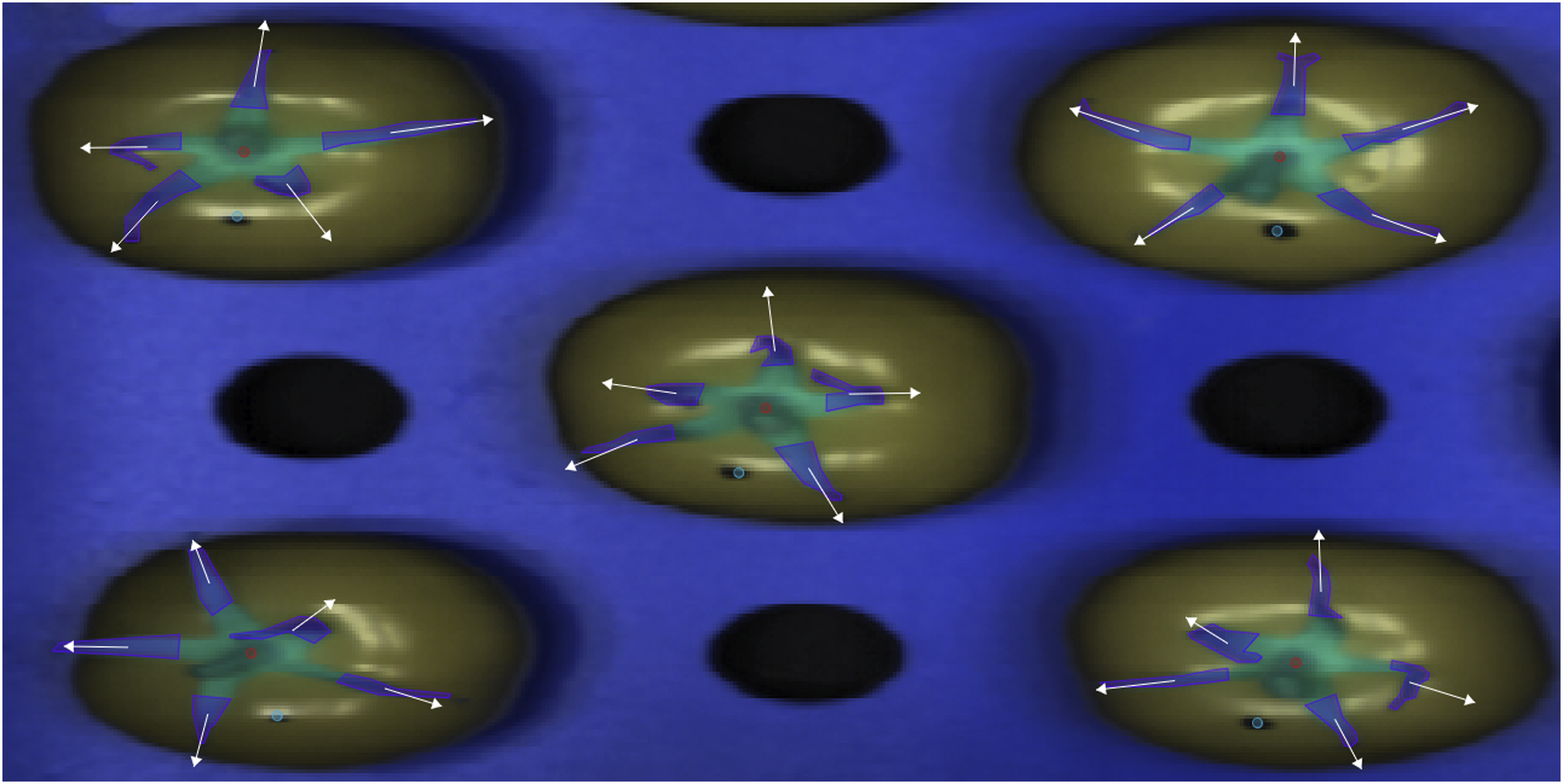
The Darwin annotation tool from V7 labs was used to perform annotations. 22 Annotations were used to extract sepal pixel spectra using a custom Python image processing pipeline employing the Numpy and Pandas libraries. The extracted sepal pixel spectra were made available for the R pipeline in spreadsheet format. 23
Data analysis
A chemometric analysis was conducted with the aim of calibrating and validating models to predict the susceptibility to fungal infection in tomatoes according to their degree of disease as observed by specialists after 4 days of germination. This analysis was done using R Statistical Software (v4.3.0; R Core Team 2021) with caret, rchemo and prospectr packages, and involved the following steps:24–27
Data visualization
Firstly, spectra were plotted to have a first appreciation of the shape of the data, observe their clarity, signal-to-noise ratio, presence of obvious outliers, baseline, etc.
Data exploration and outlier removal
Burger found that bad pixels exhibit significantly different spectra compared to their neighbors. These abnormal pixels were classified into “dead pixels,” which do not respond to light, “hot pixels,” characterized by high dark current, and “stuck pixels,” which maintain an almost constant intermediate value. Liu further explained that hot pixels have a higher dark current than normal pixels, which experience a moderate dark current increase after irradiation. Moreover, some pixels are always noisy, while others are noisy only sporadically; some may show a “non-linear response to light intensity” while some others behave randomly. 28 In any case, these abnormal pixels exhibit distinct behavior compared to the rest and thus should be removed.
In this study, all pixels of a sepal were subjected to exploratory analysis using principal component analysis (PCA) at both the sepal and variety levels. During this process, any pixels presenting anomalies, such as being out of focus, were detected and removed before averaging all pixels of a sepal. This procedure served as a robust quality control measure, aimed at identifying and eliminating spectra that are out of focus or of poor quality.
In this step, PCA was applied over all the pixels for a given sepal. To detect outlier pixels, Mahalanobis distances were computed between the individual projection of each score value onto the model and the center of the model. The identification of outliers was determined based on a specified confidence level (0.95), indicating the probability that a data point lied within a certain range. The cutoff for Mahalanobis distances was employed as a threshold, beyond which data samples were classified as outliers. The confidence level played a crucial role in controlling the sensitivity of the outlier detection, with higher confidence levels leading to more stringent criteria for identifying outliers.
Once the outliers were removed, the remaining pixels were averaged, and the datasets were finally reassembled according to their labels. Consequently, data exploration was carried out again by PCA in order to remove outliers at variety level (in Provine, Brioso and Cappricia datasets). Score plots were created, outliers were detected visually and removed from the dataset.
Pretreatments on raw spectra
Different models were calibrated and validated using various pretreated forms of the original spectra, and their performances were compared. These methods include: Detrend grades 1 and 2; Savitzky–Golay first and second derivatives, second polynomial degree and either 9-, 11-, 15-, or 17-point smoothing windows; standard normal variate (SNV); and combinations of these.29–31 Only the best results are presented.
Data split
Three binary-class scenarios were derived from the visual expert scoring described in the data collection section: - Scenario 1: Score of 0 was considered healthy, and any other value was considered infected. - Scenario 2: A score of 1 or less was considered healthy and the rest infected. - Scenario 3: Scores from two consecutive days were averaged, and samples were considered healthy when the score was 0.5 or lower, otherwise the sepal was considered infected.
Stratified sampling was carried out in the following way. Each dataset was divided into calibration (70%) and validation (30%) sets, in a representative way for each class, randomly. This means that the 70/30 ratio was respected in both classes.
Feature selection
An iterative process was used to select a sparse subset of important variables from the training set, using CovSel algorithm.32,33 Iteratively top 5 to top 39 important variables (ivs), (numbers chosen arbitrarily), were chosen for each pretreatment, labelling and cultivar. The selected variables were then used as input for the classification model, and saved in a matrix called “CovSelTrain”. The same ivs were selected from the test Set, and saved in “CovSelTest.”
Calibration and validation of PLSDA models
The Training set was split again, into calibration (70%) and validation (30%) sets, randomly. Different models with different number of latent variables (LVs) were calibrated in the calibration set and tested in the validation set. The number of LVs was selected according to the model that showed the lowest prediction error in the validation set.
All models calibrated in the calibration set must be tested (validated) later, in the validation set. A model might yield exceptional and highly accurate outcomes when applied to the calibration set. However, if overfitting occurs, the same model may produce poor results when evaluated using the validation set. In other words, an overfitted model fits perfectly well the calibration set, but cannot be generalized for efficient use in new, unknown samples.
To avoid this, the optimal number of latent variables must be chosen, according to the error observed in the validation set, when the model is tested on independent samples, which were not used during its calibration.
The prediction error in the calibration set can always decrease, carrying a risk of overfitting. Instead, the prediction error in the validation set decreases up to an optimal number of LVs, after which it increases. At this inflection point the optimal number of LVs that should be chosen for the model can be known. If a greater number of LVs is chosen, the model will have a risk of overfitting.
In other words, for each latent variable number, a prediction error value is obtained in the validation set. It is necessary to know all the prediction error values that correspond to all the different numbers of Lvs and choose the one that entails the smallest prediction error, in the validation set.
The PLSDA model, already optimized for the number of latent variables, was tested in “CovSelTest,” and classification parameters were obtained.
Evaluation of results
Parameters commonly used to evaluate classification models.
TN: true positives; TN: true negatives; FN: false negatives; FP: false positives.
Source: Akosa, 2017.
The iterative process carried out in this work can be summarized as follows: A. Spectra visualization and outlier removal. B. Model selection. 0. Start with a cultivar from a set of cultivars. Start with no “best model” for the cultivar. 1. Select labelling scenario (from 3 scenarios). 2. Select one pretreatment or combination of pretreatments; 3. Split dataset. 4. Select important features. 5. Apply PLSDA and select the optimal number of latent variables (LVs). 6. Repeat Steps 4 and 5 selecting from 5 to 39 variables by CovSel. 7. If a model BA is higher than the previous model, keep the current model as the “best model.” Note: Results of steps 1 to 7 will give the best model per cultivar. C. The same process was repeated for global modeling (“GM”) where different scenarios of variety combinations were investigated: Cappricia + Provine, Cappricia + Brioso, Brioso + Provine and Cappricia + Provine + Brioso.
Results and discussion
Average of the pixels coming from the region of interest (ROI)
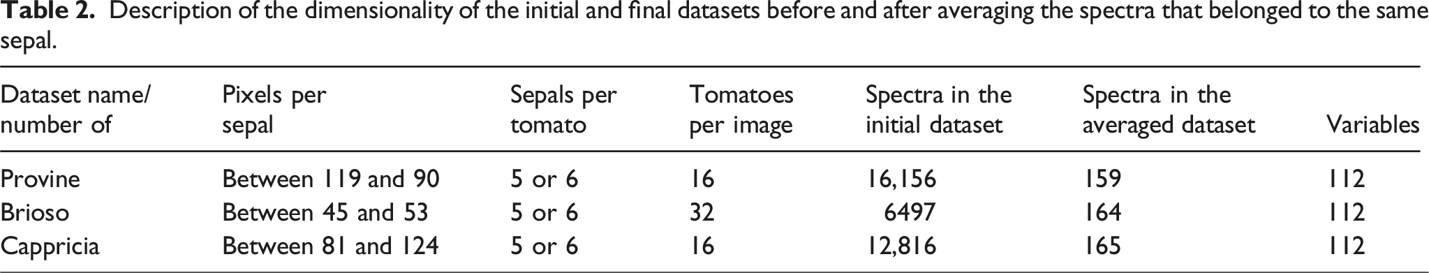
Description of the dimensionality of the initial and final datasets before and after averaging the spectra that belonged to the same sepal.
Interpretation of raw spectra
Three bands were observed in the pure and pretreated spectra of all varieties (Figure 2(a) and (b)). In the following paragraphs, tentative assignments will be mentioned along with their bibliographic sources. Raw (a) and SNV and second derivative (2, 17, 2) spectra (b) for each variety.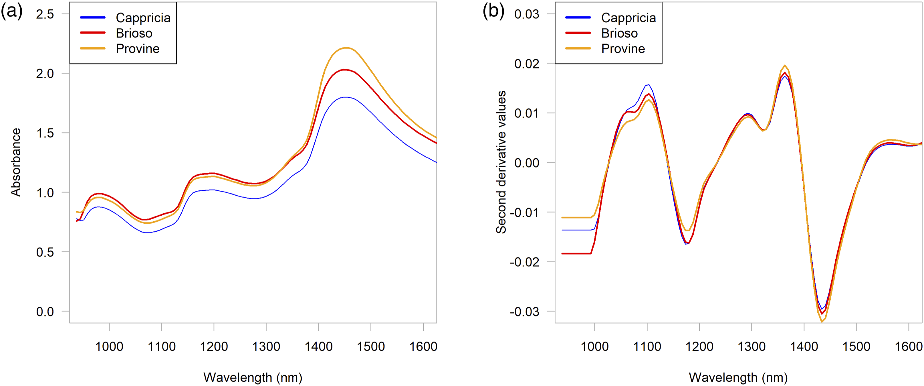
The maximum intensities observed were 1.80 (Cappicia), 2.21 (Provine) and 2.03 (Brioso); at 1455 nm (6873 cm−1) in Cappricia and at 1448 nm (6907 cm−1) in the other two varieties. These bands can be attributed to the symmetric and asymmetric stretching vibrations of water molecules at the first harmonic of the OH stretching vibrations of water. 36 More specifically, those wavelengths are included into two well-defined wavelength ranges where water shows the greatest variation of energy absorbance in response to disturbances, (Water Matrix Coordinates, “WAMACS”), called C8 and C9. “WAMACS describe different conformations of water such as water dimers, trimers, superoxides, water solvation shells, etc.”36,37
C9 1458-1468 nm: Water molecules with 2 hydrogen bonds (S2)
C8 1448-1454 nm: ν2 + ν3, Water solvation shell, OH-(H2O)4,5.37,38
The other peak in raw spectra was located at 1195 nm (8368 cm−1) in all three varieties. According to Jakubíková et al. “The region from 8300 to 8600 cm−1 corresponds to the third overtone band of the bond CH.” 38
Dalimov et al. concluded that tomato has approximately 11% lignin with carboxylic groups that distinguish it from other plants. 28 Moreover, these authors analyzed IR spectra of suspended tomato particles, and found typical absorption bands for lignin and carbohydrates. They assigned the 1195 nm wavelength to the second C-H stretching overtones of methyl groups, CH3-groups, as well as the lignin component of tomatoes.
However, other publications assigned this band to glucose. Tanaka et al. measured several glucose anomers in light and heavy water by NIR, and found a peak at 1195 nm in both solvents. 39 Furthermore, Lopez et al. performed carbohydrate analysis by NIR, and assigned the same peak to the OH stretch 1st overtone of glucose. 40
Finally, the three raw spectra have a peak at 979 nm (10,242 cm−1). It has been assigned in literature to the O–H stretching second overtones, to the hydroxide ion (980 nm) and to the hydrogen-bonded –OH, 2nd overtone (980 nm).41,42
Pretreatments and exploratory analysis
First, the raw spectra were plotted after being extracted from the images. This first visualization allowed us to have a first appreciation of how the spectra looked in relation to noise and scattering effects, distortions in the baselines, signal-to-noise ratio, in addition to the presence of clear outliers. To understand the presence of multiplicative and/or additive effects in the spectra, their intensities were plotted as a function of the average spectra (graphs not shown here). The shape of these graphs (millefeuille or cone) helped distinguish effects in the spectra. In all cases, combined effects (multiplicative and additive) were found in the analyzed spectra. Figure 2(a) shows the average of the raw spectra for each variety, and Figure 2(b) shows the average of the spectra pretreated with SNV and second derivative (17-point window, 2nd order polynomial fit). As mentioned above, other pretreatments were applied and compared as well. It should be mentioned that in this study, the most appropriate pretreatments were chosen according to the way in which they modified the performance of the models.
In this example, SNV was used to remove both the scattering effects caused by the diffusion of photons and the measurement noise (random phenomena present throughout the entire measurement chain). The resulting spectra had media equal to zero and standard deviation equal to one. Furthermore, the second derivative allowed to find the exact location (center) of the shoulders in the original spectra, by deconvoluting and highlighting the peaks. As a result, significantly narrower bands were observed. The peaks appeared in the same locations as the peaks in the original spectra.
The PCA analysis was performed in this case on the pretreated spectra, first with SNV and then with the second derivative (17-point window, 2nd order polynomial fit), in all three varieties.
When examining all three varieties together using PCA, discernible clustering patterns did not emerge (Figure 3). The analysis indicated that the cumulative variance explained by the first 20 principal components accounts for approximately 99.6% of the total variance. Specifically, the first principal component (PC1), the second principal component (PC2), and the third principal component (PC3) represented the most significant contributors to this cumulative variance, explaining 45.5%, 24.6%, and 10.4% of the total variance, respectively. Subsequent components gradually contributed smaller proportions of variance, with PC20 explaining 0.1% of the total variance. Despite the comprehensive coverage of variance by the first 20 components, no distinct separation between the varieties was observed in the PCA plot, suggesting considerable overlap in their underlying characteristics. PCA score plots of three sample groups (Cappricia, Brioso, Provine): (a) PC1 vs PC2, (b) PC2 vs PC3, (c) PC1 vs PC3, (d) PC1 versus PC4.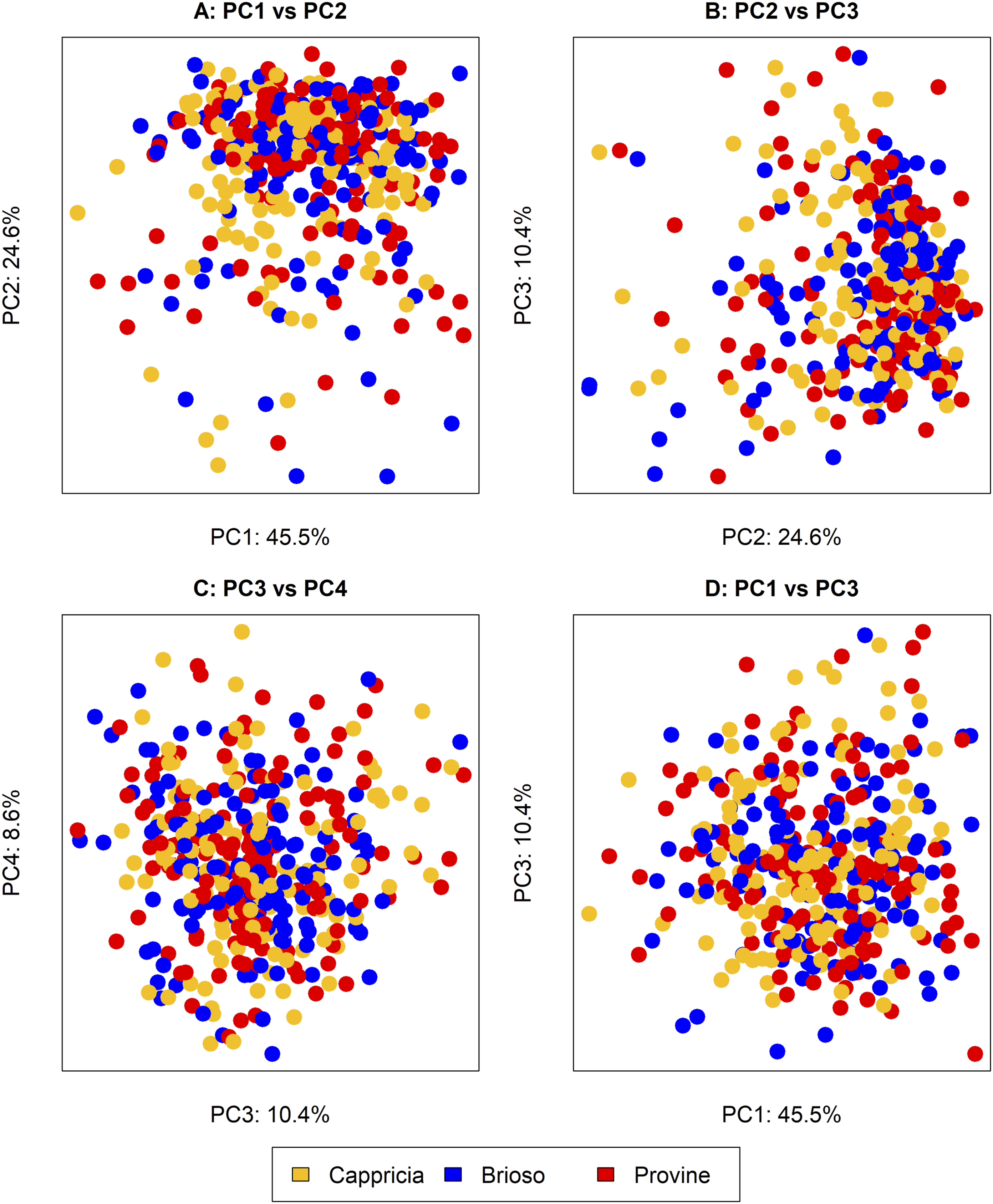
Results of exploration by PCA, to detect outliers at cultivar level.
As previously mentioned, principal component analysis was conducted individually for each variety, as well as collectively for all varieties combined. Opting for the former approach afforded a more nuanced understanding of the intrinsic variability inherent to each distinct variety. The focus centered on elucidating the important wavelengths showed by the loadings of the initial three principal components (PC1, PC2, and PC3). It is worth noting that while the analysis predominantly relied on these three components, a more comprehensive examination necessitated a greater number of components to adequately account for the variance observed within each dataset. For instance, in the case of Cappricia, 99.0 % of the variance was explained by 7 PCs, Provine exhibited 99.1% variance explained by 8 PCs, and Brioso manifested 99.2% variance explained by 8 PCs.
These loadings represented the correlation between the original variables (wavelengths) and the principal components. Loadings of greater magnitude indicated stronger correlations between the variables (wavelengths) and the principal components. The sign of the loadings indicated the direction of the correlation. Positive loadings indicated a positive correlation between the wavelength and the principal component, while negative loadings indicated a negative correlation.
PC1 loadings highlighted distinct wavelengths across the three varieties (Figure 4). Between 1034 nm and 1132 nm, Cappricia and Brioso exhibited notable wavelengths, while Provine showed a key wavelength at a lower intensity. Cappricia displayed a significant wavelength at 1251 nm. In the range from 1300 nm to 1400 nm, all three varieties presented key wavelengths. Lastly, in the 1400 to 1500 nm range, Brioso had peaks at 1420 nm and 1505 nm, while Cappricia showed peaks at 1413 nm and 1512 nm. PC 1 Loading plots of cultivars Cappricia, Provine and Brioso.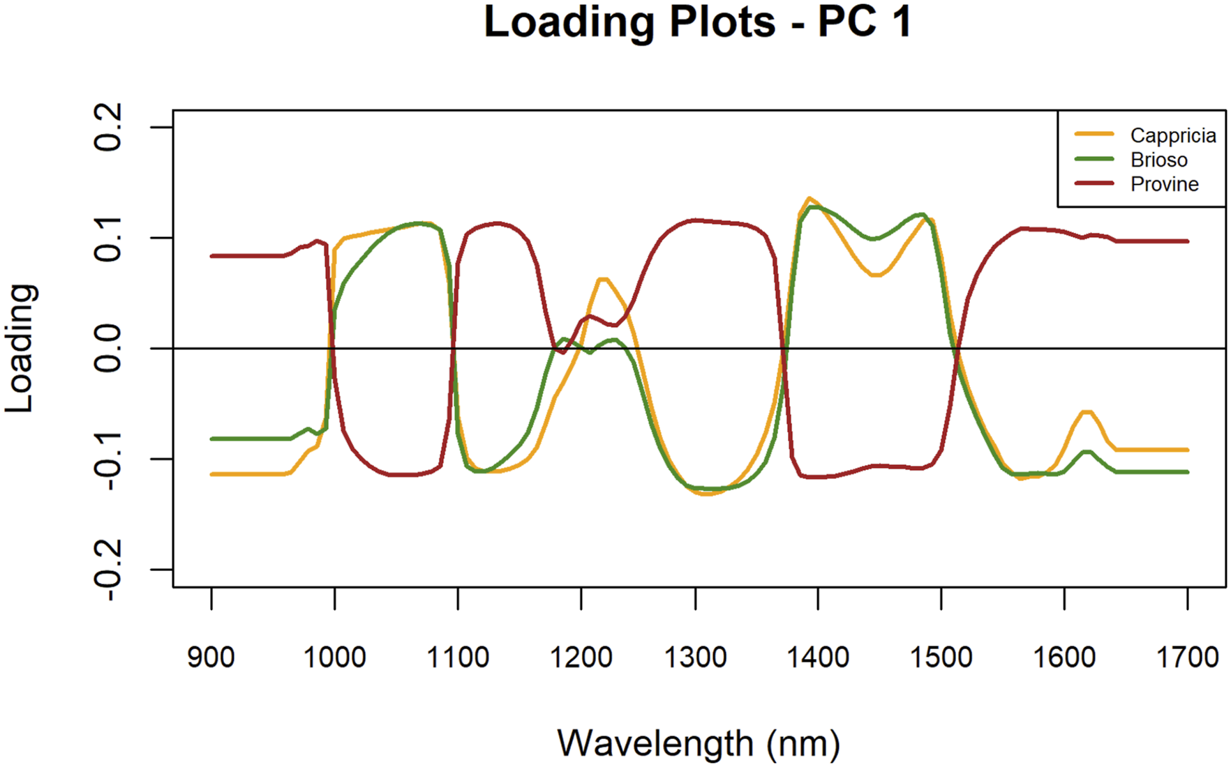
Similarly, PC2 loadings showed shared peak positions among the varieties (Figure 5). Each variety exhibited a peak at 1034 nm, while all three varieties presented notable peaks at 1258 nm, 1391 nm, and 1469 nm. Between 1500 nm and 1600 nm, Brioso showed defined peaks at 1533 nm and 1633 nm, with Provine peaking at 1554 nm and 1618 nm. Cappricia also aligned with Brioso at 1533 nm and 1633 nm. Starting from 1300 nm, the intensity range was more constrained for Provine (0.32329) than for Brioso (0.35), highlighting distinctions in spectral intensity ranges among the varieties. PC 2 loading plots of cultivars Cappricia, Provine and Brioso.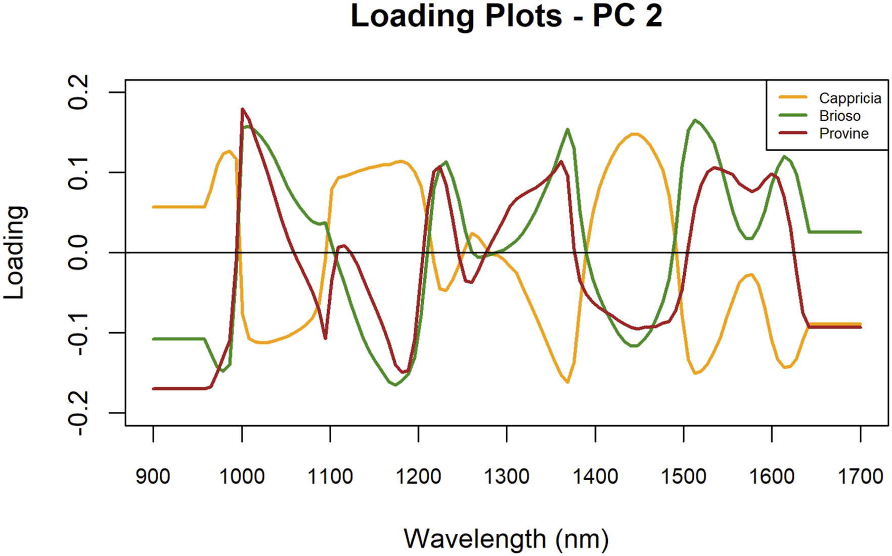
In addition, the analysis of PC3 loadings identified unique peak positions for each variety (Figure 6). Brioso exhibited peaks at 1027 nm, 1146 nm, 1244 nm, 1335 nm, 1462 nm, and 1611 nm. Cappricia showed peaks at 1209 nm, 1363 nm, and 1583 nm, while Provine presented peaks at 1209 nm, 1391 nm, and 1540 nm. These distinct wavelengths highlight the spectral characteristics of each variety based solely on peak positions. PC 3 loading plots of cultivars Cappricia, Provine and Brioso.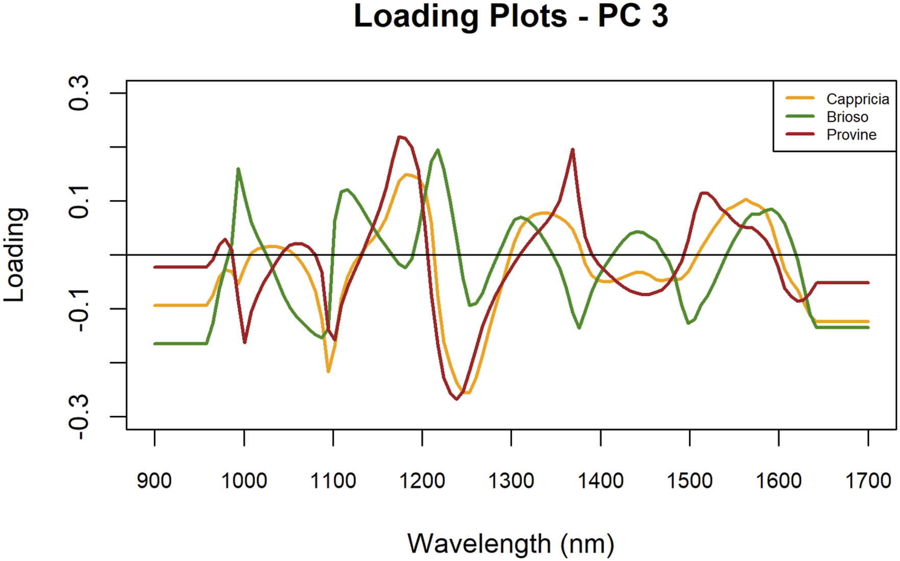
In summary, each tomato variety demonstrated distinct spectral patterns across PC1, PC2, and PC3, highlighting unique characteristics that may be influenced by NIR wavelengths. PC1 revealed notable differences in Cappricia, suggesting distinctive biochemical or structural components relative to Brioso and Provine. PC2 showcased spectral features that set Provine apart, indicating specific biochemical markers or metabolic traits distinguishing it from the other varieties. Lastly, PC3 emphasized unique spectral properties primarily in Brioso, marking characteristics less evident in Cappricia and Provine. These findings underscore the potential for NIR wavelengths to differentiate tomato varieties based on their spectral profiles.
Data split
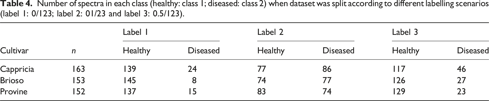
Number of spectra in each class (healthy: class 1; diseased: class 2) when dataset was split according to different labelling scenarios (label 1: 0/123; label 2: 01/23 and label 3: 0.5/123).
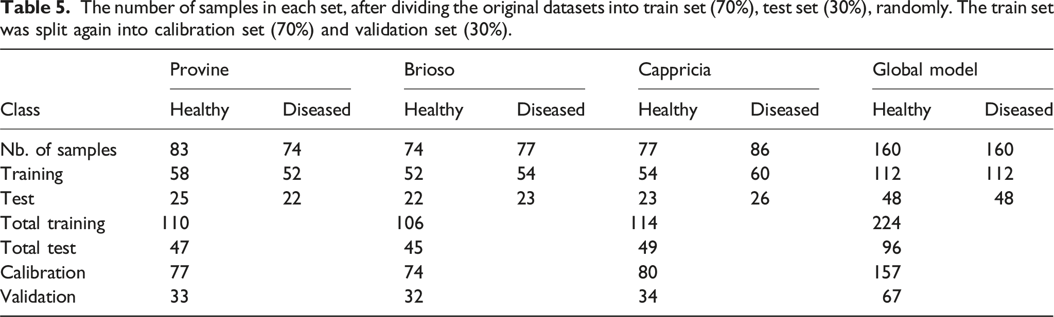
The number of samples in each set, after dividing the original datasets into train set (70%), test set (30%), randomly. The train set was split again into calibration set (70%) and validation set (30%).
Classification
Intravariety models
Different results obtained using different labeling scenarios between the healthy and the diseased classes for Cappricia cultivar were compared (plots not shown). As a result, the precision metric behaved erratically when Scenario 1 was selected. This metric showed high values when less than 13 variables were chosen, but then decreased abruptly with 14 variables; and increased again when 15 variables were chosen. This counterintuitive behavior was due to the fact that the precision metric took into account false positives in the denominator, which changed abruptly with different splits. In other words, the behavior of the precision metric showed that the data were not uniformly distributed in both classes, when Scenarios 1 and 3 were chosen. Another indicator of class balancing was the correlation between the accuracy and the balanced accuracy. When the classes were balanced, these metrics were almost identical, and their lines overlapped as observed in Scenario 2. On the other hand, a clear separation was observed between them, the accuracy was higher than the BA (graph not shown).
As a rule, high BA values showed that the model performances were good for both classes. On the other hand, high accuracy metric showed that the model performed well, in general, given the existing dataset balance. When using Scenarios 1 and 3, this was the case only for the majority classes.
It should be mentioned that there are several ways to solve data imbalance. One of them is oversampling (adding samples from the least represented class); another one is undersampling (deleting samples from the majority class). In the first case, poor implementation risks overfitting, the risk of overfitting increases, since during cross-validation, the same samples that are in the model can be used to validate it. In the second case, important information can be removed from the model.
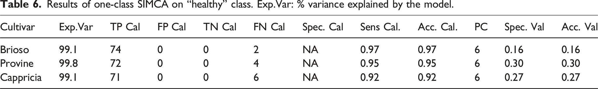
A one-class classification could also have been used, where all samples similar to the samples of one class are included, and the others discarded by the model. However, these models are always less specific, and in the case of the present study, they showed poorer classification metrics.
Results of one-class SIMCA on “healthy” class. Exp.Var: % variance explained by the model.
Due to these reasons, Scenario 2 was chosen to calibrate and validate the models. No addition or removal of samples was made, except for the aforementioned outliers.
The relationship between BA and ivs can be seen in Figure 7, for the different Scenarios 1, 2 and 3, in the Cappricia model. Once again, we can see that Scenario 2 was the best option, because it showed higher BA values. Comparison of balanced accuracy in different labelling scenarios according to different number of important variables as input for PLSDA, in the Cappricia model.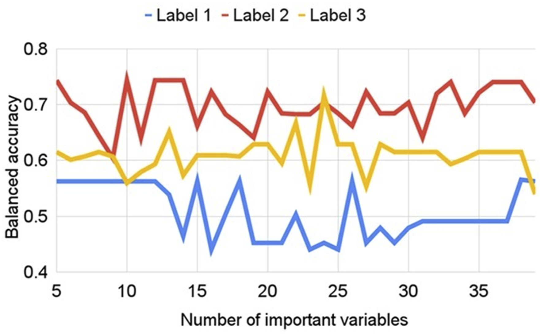
Another interesting aspect to highlight in Figure 7 is that the model’s performance remained the same with 5 variables as it did with 37 or 38 variables. This indicated that a smaller subset of variables captured the essential information needed for classification, making the model more efficient without significantly compromising accuracy. Specifically, for Cappricia, the 5 most influential variables chosen by CovSel were: 959 nm, 1000 nm, 1097 nm, 1441 nm, and 1654 nm. It is interesting, therefore, to analyze what these variables brought and what the NIR was sensitive to in this case.
In a general sense, NIR spectroscopy is particularly sensitive to overtones and combination bands of fundamental molecular vibrations, primarily involving C-H, O-H, N-H, and S-H bonds. The spectral assignment of the specified wavelengths were elucidated through their association with various molecular vibrations and the corresponding chemical compounds. The wavelength at 959 nm was related to the first overtone of C-H stretching vibrations, commonly found in hydrocarbons, lipids, and fatty acids. 43 At 1000 nm, a region that corresponds to harmonic combinations of C-H and O-H stretches, as well as overtones of C-H bonds in methyl and methylene groups was observed. This wavelength was often linked to carbohydrates, proteins, and alcohols. 44 The wavelength of 1097 nm was linked to the first overtone of O-H and N-H stretching vibrations, indicating the presence of water, proteins, and amines. 45 The 1441 nm wavelength corresponded to a combination of O-H stretching and bending bands, commonly found in water and alcohols. It was also sensitive to the hydrogen bonding in these compounds.44 Finally, the wavelength at 1654 nm was associated with combination and overtone bands of N-H stretching and bending vibrations, along with potential C-H combinations, indicative of proteins, amides, and organic compounds containing nitrogen.46
Achieving a balance between optimizing the model to achieve the highest statistical parameters and a more efficient model in terms of complexity but with slightly lower performance is always necessary. It is therefore worth noting that while the model with 5 variables was more efficient, the optimized model required 33 variables. This underscored the trade-off between model complexity and efficiency, where the choice depended on the specific requirements and priorities of the analysis.
Optimal models were generated using different parameters for each tomato variety: for Cappricia, SNV pre-treatment along with second derivative2,15 and 33 independent variables (ivs) were employed; for Provine, SNV with 13 ivs was applied; while for Brioso, raw spectra with 18 ivs were used.
Global models
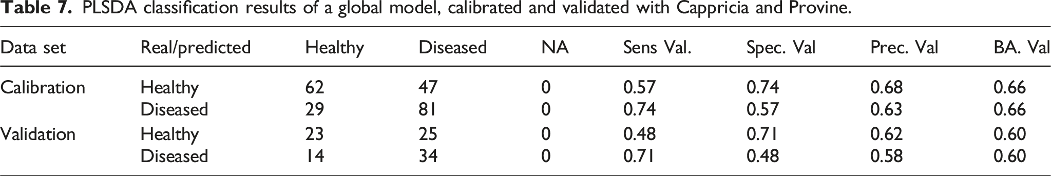
PLSDA classification results of a global model, calibrated and validated with Cappricia and Provine.
PLSDA classification results of all the optimal models in this study.
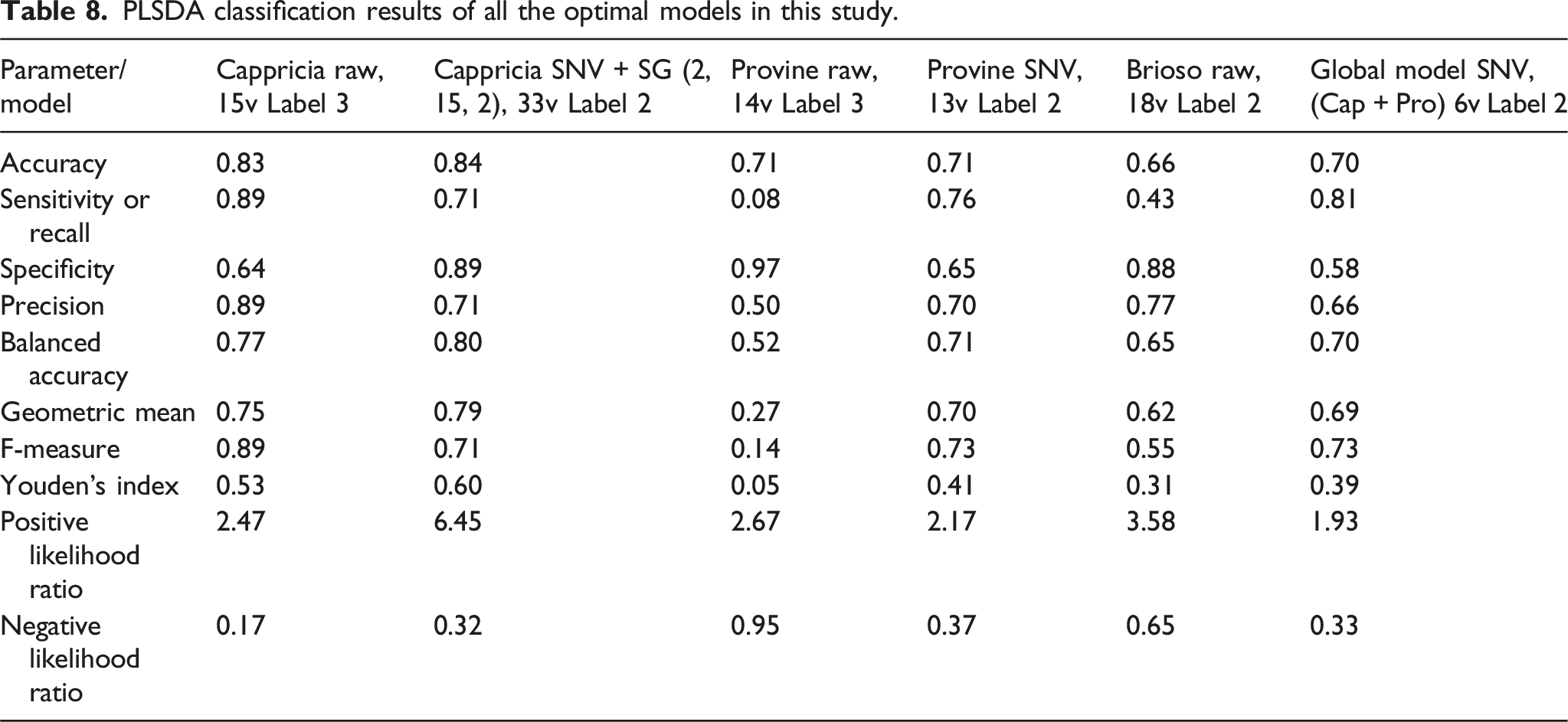
Accurate predictions for healthy sepals (sensitivity) were as follows: Cappricia (0.71), Provine (0.76), GM (0.81). Similarly, for diseased sepals correctly classified as such (specificity): Cappricia (0.89), Provine (0.65), GM (0.58).
Moreover, good performances on both positive and negative classes were found in the Cappricia Intravariety model. High positive likelihood ratio of 6.45 (above 1: increased evidence for disease-free) for the Healthy class; Low negative likelihood ratio of 0.32 (increased evidence for disease) for the Infected class.
For two-class classification, the geometric mean was calculated as the square root of the product of specificity and sensitivity (Table 1). As a rule, if one of the classes cannot be recognized by the model, the geometric mean tends to zero. 47 This parameter showed this behavior, when its values were less than 0.5. This was observed in the case of sample classification of the Provine variety using Scenario 3. Although the specificity of this model was high, the sensitivity was very low (0.08), and the geometric mean was 0.28. In all other cases, this parameter was greater than 0.5 showing that the models were able to recognize both classes.
Interpretation of information conveyed by PLSDA loadings
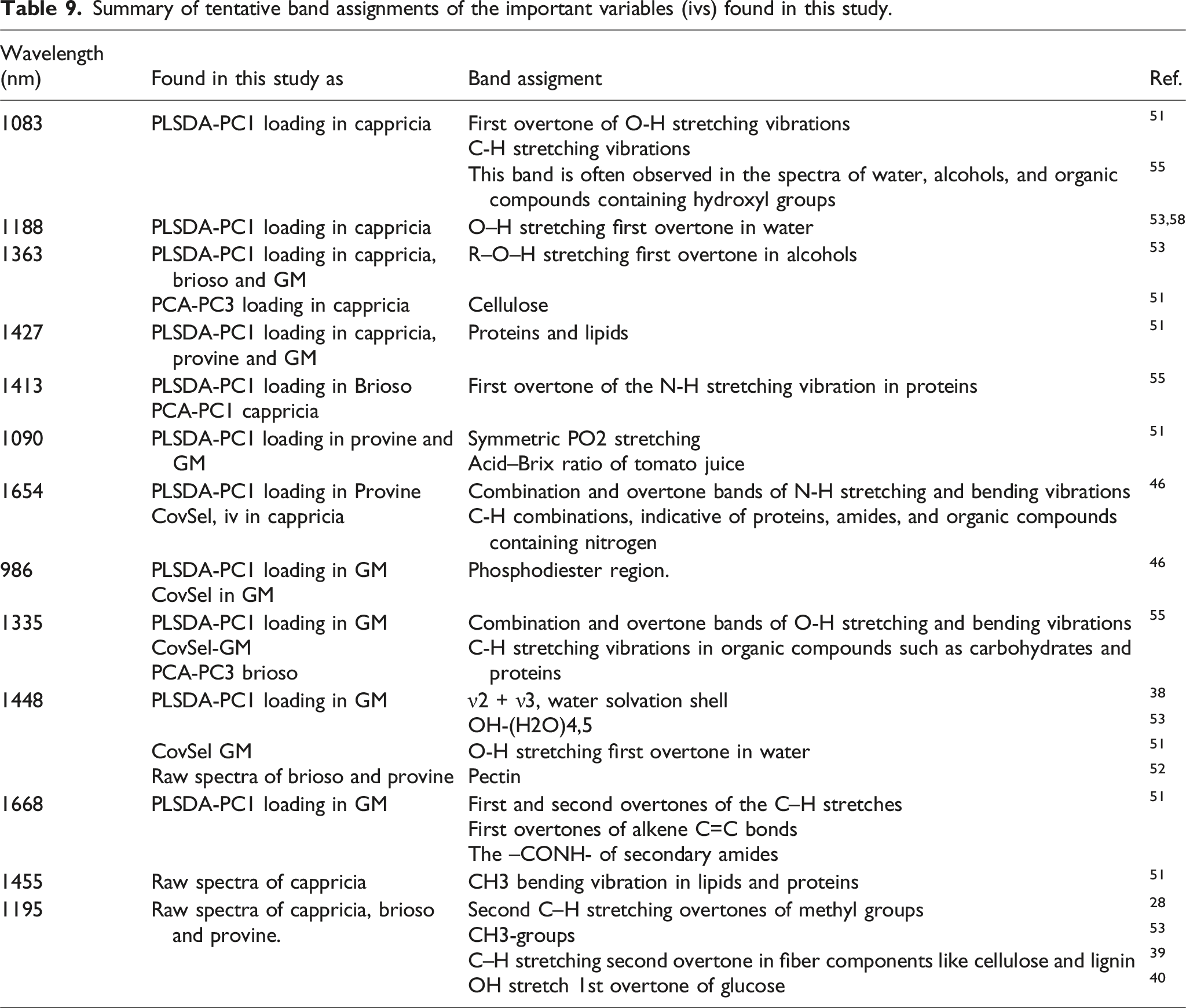
Out of the 33 variables selected by CovSel in the Cappricia model, PLSDA assigned greater importance to 1083 nm (iv 7), 1188 nm (iv 10), 1363 nm (iv 18), and 1427 nm (iv 21), according to the loadings of its first principal component.
In the Brioso model, 18 variables were selected by CovSel, with PLSDA also emphasizing 1363 nm (iv 7), similar to Cappricia, indicating its relevance to the susceptibility of tomato sepals. Additionally, PLSDA placed emphasis on variable number 9, at 1413 nm, which represents an important feature in Brioso sepals, aiding in their distinction from other varieties.
Regarding Provine, 13 variables were selected by CovSel, and among them, the PLSDA model for classification utilized 1090 nm (iv 6), 1427 nm (iv 8), and 1654 nm (iv 10). Interestingly, wavelength 1427 nm (iv 8) was common between Provine and Capprica, indicating its significance across multiple varieties.
In the GM with SNV, comprising the 37 most important variables according to CovSel, the key ones were five: 986 nm (iv 5), 1090 nm (iv 9), 1335 nm (iv 15), 1448 nm (iv 20), and 1668 nm (iv 31). It is worth noting that the 1363 nm wavelength (iv 18) was common among Capprica, Brioso, and the GM, while the 1427 nm wavelength (iv 21) was common between Capprica, Provine, and the GM.
Several reasons explain the selection of specific wavelengths by PLSDA models. According to Silva et al. in 2020, the factors contributing to tomatoes’ susceptibility to fungal diseases include the abundance of simple sugars and organic acids, or the activity of host cell wall-modifying proteins. 48 These factors, combined with the presence of water and environmental conditions, elucidate why the selected wavelengths played a significant role in the classification studied in this work.
It is worth noting that natural defenses in fruit, like cell walls, waxy coatings, and the skin, provide inherent resistance. When an infection takes place, the fruit initiates various systemic signals that activate specific defenses against the pathogen, thus safeguarding other parts of the fruit. The stage of ripeness determines the type of defense compounds present in the fruit. Nonetheless, some pathogens can bypass these defenses and cause infections, highlighting the importance of the composition of ripe fruit in the emergence of post-harvest diseases. 49
As mentioned earlier, the raw spectra showed bands at approximately 979 nm, 1195 nm, 1448 nm, and 1455 nm. These bands were also observed in similar wavelengths (970 nm, 1446 nm, and 1200 nm) by Li et al., who estimated the sensory qualities of tomatoes using visible and near infrared spectroscopy. 50 These authors attributed the 970 nm band to water and the 1190 nm band to the second overtone symmetric stretch of methyl groups. 48
Furthermore, the bands at 970 nm, 979 nm (or 978 nm), 1188 nm (or 1190 nm), and 1448 nm (or 1450 nm) have been attributed to the O-H stretching first overtone in water by several authors.51–53 According to de Brito et al. the peak at 979 nm (or 978 nm) is caused by water due to its relation to the O–H absorption band range (740 nm, 840 nm, 960 nm, and 1440 nm). 51 Similarly, the bands at 970 nm, 1188 nm (or 1190 nm) and 1448 nm (or 1450 nm) were attributed to the O–H stretching first overtone in water.52,53
The water content in tomato sepals can affect their susceptibility to fungal attacks. 54 High moisture levels in plant tissues, including sepals, can create a favorable environment for fungal growth and infection. Fungi, such as Botrytis cinerea (grey mold) and A. alternata, thrive in humid conditions where water availability facilitates spore germination and mycelial growth. 55 Spores of many pathogenic fungi require high humidity conditions to germinate. The presence of water in plant tissues, including sepals, provides the moist environment necessary for spores to activate and begin germinating. 38 According to Thomma, some spores require high humidity to germinate and penetrate plant tissues. 56 Elad et al. emphasized that water content and humidity levels can significantly impact the resistance or susceptibility of tomatoes to fungal infections, as fungi like Botrytis cinerea require moisture for spore germination and infection establishment. 57
Secondly, polysaccharide and saccharide levels contribute to tomatoes susceptibility to fungi. 48 Peaks for polysaccharides and/or saccharides (at 1170 nm and 1200 nm) were used to differentiate tomatoes of different ages, indicating postharvest ripening levels regardless of storage conditions. 52 Blanco et al. found that the polysaccharide content in tomato stem tissues significantly affects the susceptibility of tomatoes to Botrytis cinerea infections. Research has shown that these compounds play crucial roles in the structural integrity and biochemical properties of plant tissues, thus affecting their interactions with fungal pathogens. Tomato sepals, like other plant tissues, are composed of cells with cell walls containing polysaccharides. These polysaccharides contribute to the structural integrity of the sepals and play a role in their defense against pathogen invasion.38,55 By fortifying the cell wall, polysaccharides in tomato sepals enhance their resistance to fungal pathogens. A robust cell wall can impede the penetration of fungal hyphae or spores, limiting their ability to infect the sepals and cause disease. 38 According to Jones and Dangl, during pathogen invasion, fungal pathogens attempt to penetrate the plant cell wall to gain access to nutrients and cause disease. Polysaccharides play a vital role in strengthening the cell wall, making it more resistant to penetration by fungal hyphae or spores. This reinforcement of the cell wall serves as a physical barrier that impedes the progress of fungal pathogens, thereby enhancing plant defense mechanisms. 58
Moreover, tomato sepals contain various sugars such as glucose, fructose, and sucrose, which can serve as energy sources for fungi. The 1170 nm band is associated with the C–H stretching second overtone bonds, indicating the presence of carbohydrates in fruit. Furthermore, Blanco et al. indicated that NIR data between 1069 and 1125 nm, specifically at 1083 nm and 1090 nm in this current research, have been used to predict the acid–Brix ratio of tomato juice. Regarding the 1668 nm band, it has previously been assigned to the first and second overtones of the C–H stretches, the first overtones of alkene C=C bonds, and the -CONH- of secondary amides. 51 These functional groups, such as cis-RCH=CHR,’ CH, aromatic, and CH3, are associated with sugars, fruit acids, and some amino acids. 50
On the other hand, loadings at 1455 nm (or 1456 nm) relate to CH3 bending vibration in lipids and proteins, while a loading at 1090 nm (or 1095 nm) corresponds to symmetric PO2 stretching. 51 The 986 nm (or 981 nm) region is associated with the phosphodiester region, and the 1427 nm (or 1422 nm) band pertains to proteins and lipids. 51
The susceptibility of tomato sepals to fungal infections is significantly influenced by their lipid content. Lipids serve as essential components of plant cell membranes, affecting permeability and rigidity, which can either hinder or facilitate fungal penetration. 59 Additionally, certain lipids act as barrier components, with cuticular waxes providing hydrophobicity to prevent pathogen entry. 59 A reduction in these protective lipids can increase susceptibility to fungal infections. Furthermore, sepals possess an intricate defense mechanism that is triggered by the detection of invading pests or pathogens, leading to a series of events that may result in enhanced resistance. 60 As integral parts of cellular membranes, lipids play a pivotal role in facilitating the communication pathways that are essential for the regulation of defensive actions in plants. Research has shown that a variety of lipids, are critical in the transmission of signals during plant-pathogen interactions. 60
When it comes to proteins, Ferreira et al. described their role in plant-pathogen interactions as follows: “The interaction between a plant and a pathogen can be likened to a battle, where the primary tools used in the fight are proteins produced by both the plant and the pathogen.” 61 According to Bashir et al., the function of a cell or tissue is primarily determined by its protein composition. 62 Furthermore, a plant’s resistance to fungal infections relies on alterations in the protein composition of its cells. Upon exposure to fungal species, certain proteins stimulate the accumulation of lignin in the plant cell walls, which can strengthen the plant’s defenses against fungal pathogens. 62 Moreover, enzymes involved in lipid synthesis, such as those belonging to the phospholipase family, are responsible for generating signaling compounds that are released in response to pathogen assaults. 60
Furthermore, the 1363 nm (or 1360 nm) band is attributed to the R-O-H stretching first overtone in alcohols. 49 This spectral feature can be related to the defense mechanisms of tomato sepals against fungi because the presence of specific alcohols or phenolic compounds in the sepals, which exhibit this band, might play a role in enhancing the plant’s defenses. Moreover, they serve as precursors in the synthesis of phytoalexins, antimicrobial compounds produced in response to fungal infection, and in the formation of phenols and flavonoids, which possess antifungal properties.63,64 Alcohols also contribute to the production of lignans and tannins, which reinforce cell wall integrity and act as physical barriers against fungal invasion. 49
Phenylpropanoids, which include various chemical families such as flavonoids, isoflavonoids, stilbenes, monolignols, and lignin, function as inducible phytoalexins in many vegetable species to combat pathogens. In tomatoes, the primary phytoalexin is α-tomatine, a glycoalkaloid found throughout the plant, including the leaves, stems, and unripe fruit. Tomatine serves as a natural defense compound, protecting the tomato plant against pests and pathogens. 49 A previous study conducted by Ito et al. revealed that α-tomatine induced cell death in Fusarium oxysporum, a fungus prevalent in tomato crops. 65
Additionally, peaks related to cell wall components like pectin (1448 nm), cellulose (1363 nm), and lignin (1195 nm) are crucial. 53 Changes in these components, along with cell wall thickness during ripening, are significant. Other key peaks identified across different conditions were those relating to the structural and compositional development of the cuticle and cell wall. Compositional changes in key compounds such as pectin, cellulose, and other polysaccharides, as well as changes in cell wall thickness, are part of the ripening process. 66 Pectin undergoes de-esterification, serving as a measure of tomato maturity. Variations at 1300 nm may be due to fungal growth in inoculated date fruits, and the 1650 nm band might relate to hardness, as explained by Wang et al. for grain kernel at 1680 nm. 19 Fungal infection can alter the texture of food, making the date fruits softer as the infection progresses, a change identified at 1650 nm. 67 The 1195 nm (or 1200 nm) band is linked to the C–H stretching second overtone in fiber components like cellulose and lignin. 53
Lastly, acids like malic and citric acid altering pH, and phenolic compounds, which some fungi use as nutrients, also play roles in the susceptibility of tomato sepals to fungal infections.68,69 These organic acids can influence the pH of plant tissues. The pH can affect fungal growth and the activity of fungal enzymes. Fungi often thrive in specific pH ranges, and altering the pH of the host tissue can either inhibit or promote fungal infection. 68 Similar to sugars, citric acid declines with progressing maturation after ripening while the content of malic acid remains relatively constant. 66 Phenolic compounds are part of the plant’s defense mechanisms. However, some fungi have evolved to utilize these compounds as nutrients, potentially aiding their growth and infection processes.54,69
Summary of tentative band assignments of the important variables (ivs) found in this study.
Conclusion
This work was carried out with the objective of developing a method to predict the susceptibility of freshly harvested tomatoes to the presence of fungi, in a non-destructive way, before the disease can be observed visually. To this aim, hyperspectral images of the samples were measured, and models were developed based on their relationships with ground truth data.
The models can be divided into two general categories: those calibrated and validated using a single variety (intravariety), and those calibrated and validated with several varieties together (global models). In both cases, the best results were found using Scenario 2 as a reference.
Within the first category, the optimal model was created with the Cappricia variety: Balanced accuracy = 0.84, Sensitivity = 0.71 and Specificity = 0.89. As for the global models, the optimal models were calibrated using Cappricia and Provine together: Balanced accuracy = 0.70, Sensitivity = 0.81, Specificity = 0.58.
In this study, the significance of specific wavelengths in distinguishing tomato varieties and understanding their susceptibility to fungal infections was investigated. For the Cappricia model, PLSDA highlighted the importance of 1083 nm, 1188 nm, 1363 nm, and 1427 nm, indicating their relevance in characterizing tomato sepals’ susceptibility. Similarly, in the Brioso model, 1363 nm was emphasized, along with 1413 nm, distinguishing Brioso sepals from others. Provine model emphasized 1090 nm, 1427 nm, and 1654 nm, with the wavelength 1427 nm being common among multiple varieties. These findings were supported by previous studies suggesting that factors like sugar abundance, organic acids, water content, and environmental conditions contribute to tomatoes’ susceptibility to fungal diseases, while the presence of specific wavelengths corresponded to various biochemical and structural components in tomato sepals, such as polysaccharides, saccharides, lipids, proteins, and phenolic compounds, playing crucial roles in plant defense mechanisms and fungal infection susceptibility.
The results from this research suggest the conclusion that discrimination between more susceptible and less susceptible sepals is feasible under controlled conditions.
Footnotes
Declaration of conflicting interests
The author(s) declared no potential conflicts of interest with respect to the research, authorship, and/or publication of this article.
Funding
The author(s) disclosed receipt of the following financial support for the research, authorship, and/or publication of this article: EU Commission; 664387.