Sage Journals: Discover world-class research

Abstract

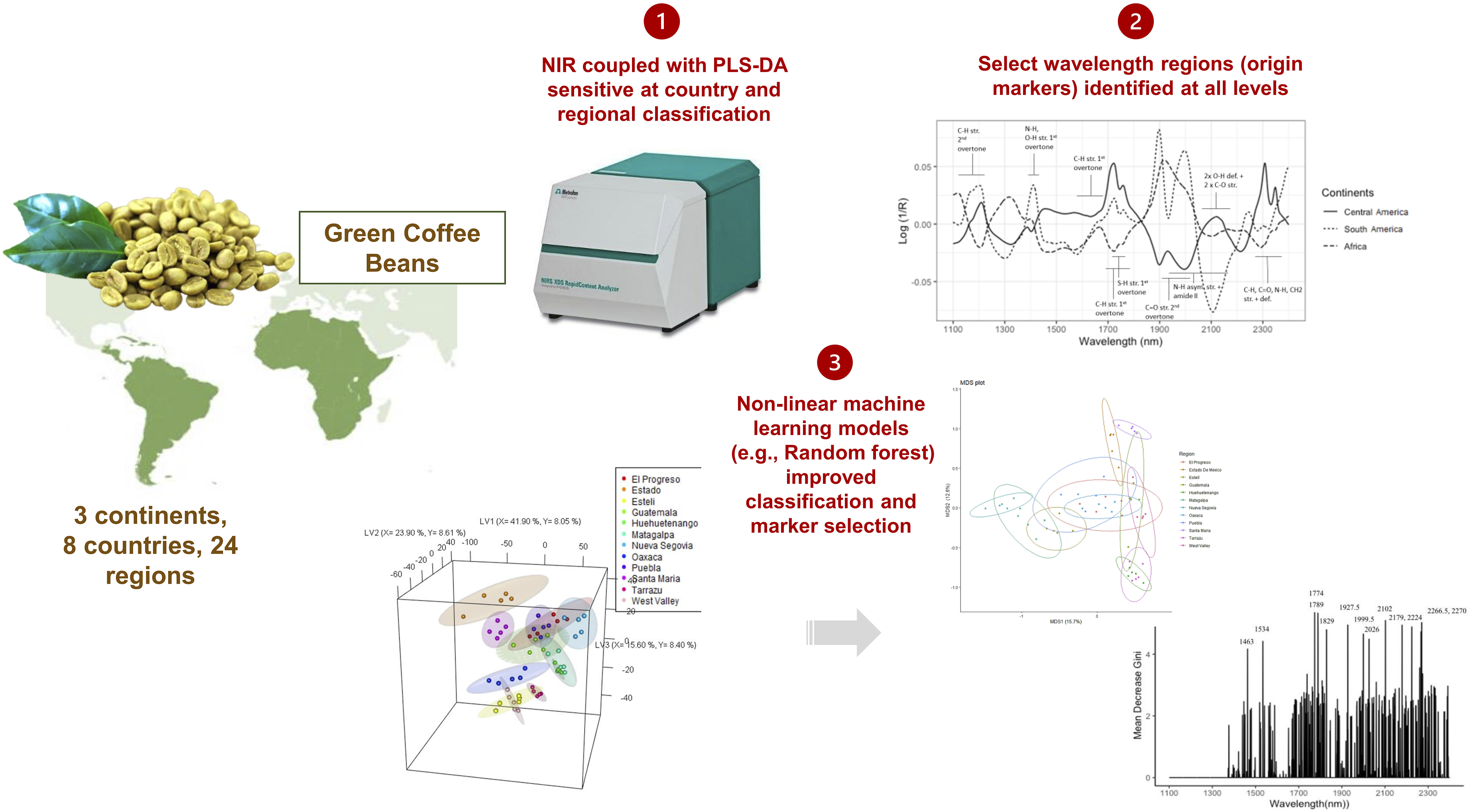
Over the past decade, there has been overwhelming interest in rapid and routine origin tracing and authentication methods, such as near infrared (NIR) spectroscopy. In a systematic and comprehensive approach, this study coupled NIR with advanced machine learning models to explore the origin classification of coffee at various scales (continental to regional level). Speciality green coffee beans were sourced from three continents, eight countries, and 22 regions. The dispersive bulk NIR spectra were used for spectral registration in the reflectance mode, and the obtained spectra were preprocessed with extended multiplicative scatter correction and mean centering. The classical linear partial least squares-discriminant analysis adequately predicted origin at the continental and country level, and showed promise at the regional level. Non-linear machine learning models improved predictions further, with the best accuracy found using random forest with accuracies up to 0.99. Discriminating wavelength regions and constituents were identified at each origin scale, with more minor wavelength regions selected by random forest. This proof of concept work demonstrated the potential of NIR spectroscopy coupled with machine learning for rapid origin classification of coffee from the continental to the regional level.

Graphical Abstract

Keywords

origin classification coffee traceability NIR machine learning PLS-DA non-linear random forest

Introduction

The last decade has witnessed overwhelming interest in the use of vibrational spectroscopy methods, such as near infrared (NIR) spectroscopy, for origin traceability and authenticity of high-value agri-food products.¹ Compared to their traditional counterparts, these methods are fast, non-destructive, and affordable. They can easily be implemented into an onsite, rapid, and robust toolbox to verify the geographical origin of high-value agri-foods, such as coffee, innovating the current less effective and slow traceability system.

Coffee is one of the high-value agri-foods frequently subjected to origin fraudulent activities due to the increasing demand for single-origin speciality coffee.² NIR spectroscopy has thus been increasingly utilised for coffee origin verification studies.³ NIR spectroscopy was used to classify and estimate diterpene concentrations in Ethiopian green coffee beans from different regions using high performance liquid chromatography (HPLC) as the reference 4. NIR spectroscopy has also been used to classify green coffee from different regions within Brazil,^5–7 and two regions in Indonesia.⁸ The spectral regions important for regional discrimination have been associated with lipids, chlorogenic acids, caffeine, trigonelline, amino acids, proteins, sugars and carbohydrates between 1400 – 2350 nm.⁵ Most coffee origin studies using NIR spectroscopy have looked at classification at the regional level. Beyond regional classification, NIR spectroscopy was used to differentiate Colombian coffee from 13 other countries (two continents) (1300 – 2400 nm).⁹ In a recent study, coffee samples from nine countries and two continents (America and Asia) were classified at the continental level using NIR spectroscopy.¹⁰

Chemometric data analysis methods are commonly used to analyse NIR spectral datasets. Nonetheless, previous studies have mainly employed linear chemometrics-based classification methods such as principal components analysis (PCA), linear discriminant analysis (LDA), and partial least squares-discriminant analysis (PLS-DA). Lately, there has been a lot of enthusiasm for using non-linear machine learning models due to their ability to handle more complex data.^11,12 These have not been well investigated, with limited understanding surrounding their use in coffee origin studies. Only one study has utilised a non-linear classifier, namely support vector machine (SVM), and demonstrated perfect (100%) prediction accuracy on four regions of coffee within Brazil using NIR spectra.⁷

The research gaps include the lack of studies investigating coffee origin at different scales, from the continental to the regional level. There is a need for more advanced machine learning models to handle more complex classification problems with a greater range of regions and levels of classification (continent, country, region). Lastly, there is a lack of studies which have identified spectral regions and their associated compounds/groups driving the classification across various scales.

This work aims to address the research gaps by investigating the potential of NIR spectroscopy for rapid origin classification of coffee at different origin scales (continental, country, regional), and for the first time, the use of four different non-linear machine learning models to improve the performance of more complex NIR problems. These modelling techniques include k-nearest neighbours (KNN), kernel support vector machines (SVM), extreme gradient boost (XGB), and Random Forest (RF). The selection of wavelength regions important for discriminating origin at the three levels will also be identified.

Materials and methods

Samples

Green coffee beans (GCBs) and metadata were obtained from Oritain Global Limited (Dunedin, New Zealand), a traceability company. The samples included 24 GCB samples originating from three continents (Africa, Central America, and South America), eight countries (Ethiopia, Kenya, Costa Rica, Guatemala, Mexico, Nicaragua, Colombia, and Peru), and 22 regions (Gedio, Guji, Maywal, Kiajibbi, Yara, West Valley, Tarrazu, Santa Maria de Dota, El Progreso, Guatemala, Oaxaca, Puebla, Estado De Mexico, Esteli, Matagalpa, Nueva Segovia, Antioquia, Huila, Narino, Cusco, Pasco). The samples were verified with certification that they were of the arabica species (Coffea arabica L.), wet-washed, and collected between 2021 to 2022 - pooled from producers in that same region and time. These samples were selected based on their importance to the coffee industry, coming from leading coffee producing continents within the coffee belt (which include 50 countries within Africa, Central America, South America, and Asia). Each sample was ground into green coffee powder (GCP) with six replicates using a liquid nitrogen mill (Cryomill, Retsch, Germany) to a particle size of 5 μm.

NIR spectral registration

A dispersive NIR spectrometer (XDS Rapid Content Analyser, Metrohm, Herisau, Switzerland) was used for spectral acquisition in reflectance mode. Approximately 2 g of powder was packed into a quartz glass vial (17.25 mm spot size) after careful mixing, with six replicates taken per sample (technical replicates). The vial was then centered onto the sampling window area, fitted with an iris adaptor, which was rotated to collect a more representative spectrum. For each technical replicate, nine analytical replicates (spectra) were obtained for a total of 1296 observations. The measurements were taken over the spectral range 1100 to 2500 nm (data sampling interval, 0.5 nm; background, 256 scans, sample, 32 scans). An instrumental internal reference standard was used for the background scan. The Vision Air 2.0 Network software (version 66072207) was used for instrumental control and spectral acquisition.

Data analysis

The spectral data were statistically assessed with R-Studio version 4.2.0.¹³ The nine analytical replicates per technical replicate were first averaged to produce six observations per sample to give a total of 144 observations.

The spectra were then preprocessed with extended multiplicative scatter correction (EMSC)¹⁴ and mean centering, which fits a second order polynomial onto the average spectrum to correct for raw spectra curvature- due to non-linearities introduced by light scatter.¹⁵ The preprocessed data was then saved for further analysis. Before modelling, the preprocessed spectra were split into training (80 %) and test (20 %) datasets using the caret (version 6.0-94) package in R, grouped by sample ID to prevent replicates splitting across the datasets.¹⁶ Cross validation (CV) was performed with a k-fold 10 data splits repeated ten times. The model performance was evaluated with balanced accuracy (Acc)^17,18 across the training, testing, and CV datasets (equation (1)).

Balanced Accuracy = \frac{1}{n} * \sum (\frac{{T P}_{i}}{{T P}_{i} + {F N}_{i}} + \frac{{T N}_{i}}{{T N}_{i} + {F P}_{i}}) / 2

(1)

Where n is the class number,

{T P}_{i}

represents the true positives for the i^th class and

{F N}_{i}

represents the number of false positives for the i^th class,

{T N}_{i}

represents the number of true negatives for the i^th class, and

{F P}_{i}

represents the number of false positives for the i^th class.

A dummy classifier also known as a random rate classifier, the no information (NR) rate, was constructed for each model to prevent overinflation of model performance using Acc. Each model was assessed to ensure its importance if Acc > NR (p-value <0.05). Compared to a random baseline, NR evaluates success in model prediction.

Linear supervised partial least squares-discriminant analysis (PLS-DA) was then conducted for the continental, country, and regional level classification. PLS-DA combines the dimension reducing ability of partial least squares (PLS) with the discriminatory capability of linear discriminant analysis (LDA)¹⁹ The spectral data was set as the X predictor, while the origin class was input as the Y response variable.²⁰ The evolution of root mean square error of calibration/train (RMSEC) and root mean square error of cross-validation (RMSECV) was used to decide on the optimum number of latent variables (LVs) used in the model. The ropls package (version 1.26.4) was used for PLS-DA in R. PLS-DA has an embedded function to relate the distribution of scores to spectral features, which can be plotted to identify the wavelength regions important for origin discrimination for each latent variable via the loading weights.^21,22

Non-linear machine learning classification models were then explored: K-nearest neighbours (KNN), radial basis function (RBF) kernel support vector machines (SVM), XGBoost (XGB), and random forest (RF). KNN measures the Euclidean distance between the observation calibration (train) and prediction (test) points.²³ K is the parameter of the nearest neighbours that is optimised based on the classification error rate and the number of observations within each class. The highest rank of the class becomes the model predicted class. The class (version 7.3-19) package in R was used to perform KNN.²⁴

The RBF kernel SVM captures non-linear relationships in the data using the RBF kernel.²⁵ The class decision boundary is optimised using the cost (C) and gamma (γ). The shape of the boundary is determined by the γ, with higher values increasing the boundary flexibility, and lower values preventing an overfit. C balances the trade-off between errors and boundary complexity, controlling the penalty for misclassification. The parameter combination was optimised with the best performance across all cross-validation rounds. Both KNN and RBF-SVM do not contain an embedded feature selection, but the genetic algorithm can be used to search for the optimum set of features that maximises classification performance in the model, but are computationally intensive.²⁶ RBF-SVM was performed using the package e1071 (version 1.7-13) with the “radial” kernel.²⁷

Both XGB and RF are ensemble decision trees which are structured like a tree where the features are the nodes, feature values are edges, and classes are leaves.²⁸ Beginning at the base of the tree, the tree branches are connected based on feature values, and the final node is the final prediction. Nonetheless, XGB and RF are distinct in their hyperparameter tuning, construction and residual treatment. XGB trees are shallow, with little depth, progressively constructed with each tree learning from the residuals of the trees before it. In RF however, each tree is constructed independently using a subset of features and the final prediction is based off the voting or average of all individual tree predictions. RF introduces randomness and diversity in feature selection with a bagging concept.

The XGB hyperparameter tuning includes the learning rate (eta), maximum depth (max_depth), number of trees (ntree), and regularisation parameters gamma (γ) and lambda (λ). Eta controls the contribution of each tree towards prediction, max_depth controls the maximum depth of every tree, ntree controls the number of boosting iterations, γ prevents an overfit using the requisite loss reduction, and λ helps to lessen the influence of individual features. The parameter combination is optimised using multiclass log loss (mlogloss). Gain is the improvement in model accuracy and the reduction in the loss function. XGB splits tree nodes up to the maximum tree depth and prunes the tree backward till there is no positive gain or improvement in model performance. In addition to the hyperparameters ntree and max_depth, RF has mtry which controls the quantity of features that are randomly selected with each tree node, thereby preventing an overfit through the introduction of diversity. These parameters are optimised through the out-of-bag (OOB) error rates that measures the predictions left out (one third of the data) and not included in bootstrap sampling during model training, providing an unbiased estimation of model accuracy.

XGB and RF contain an embedded feature selection opportunity to identify the wavelengths contributing most towards the models. XGB has an importance function which is calculated as the total gain from each tree node where the feature was utilised for splitting. Features with more importance have more influence on the model. RF feature selection is based on Gini impurity, a measure of uncertainty, it evaluates the importance of the feature by its ability to reduce the Gini impurity.²⁹ The feature with the greatest reduction in Gini impurity is most influential for class separation.

XGB was conducted using the package xgboost with the objective set to multi:softmax (version 1.6.0.1) and RF was performed with the random forest package with the tuneRF function for parameter optimisation (version 4.7-1.1).⁴²

While linear model scores can be plotted as a scatter plot to visualise model performance, more complex non-linear models operate in a high dimensional space with difficult to visualise decision boundary. To visualise the performance of the RF models, a dimension reduction step called a Multi-Dimensional Scaling (MDS) plot can be plotted.³⁰ MDS reduces the data into a two-dimensional MDS1 and MDS2 axes which perform like a conventional x and y scatter plot, providing an opportunity to estimate the underlying classification mechanisms within the model. The closer the data point is to the other, the greater their degree of similarity.

Results & discussion

Spectral features

NIR spectra are characterised by absorption bands associated with different vibrations of chemical covalent bonds. The main absorption bands are related to the composition of the bean. The mean spectra of each continent plotted after preprocessing with the associated chemical assignments are shown in Figure 1 below. The spectral pattern is in agreement with previous studies.^5,7,10,31,32 Green arabica coffee beans have been known to be dominated by carbohydrates. Specifically, the components include cell wall polysaccharides (50-60 %), galactomannans and arabinogalactan-proteins, lipids (13-17 %), proteins (11-15 %), sugars (7-11 %), and chlorogenic acids (5-8 %). Carbohydrate and sugar C-H and O-H overtones are known to dominate between 1150-1250 nm, 1400-1650 nm, 2050-2150 nm, 2250 nm, and 2350 nm.³¹ Cellulose C-H and O-H bonds signal at 1470 nm, 1780 nm, 1840 nm, and 2080 nm. Absorption bands of N-H overtones at 1450 nm, 1550 nm, 1740 nm, 2085 nm, and 2180 nm are associated with proteins and polyamides. The C-H overtones of fatty acids, lignin and amino acids signal around 1170-1220 nm, and between 1650-1750 nm. The C=O stretching overtones of esters signal around 2300 nm. Water O-H absorption bands are around 1430 nm and 1886-2000 nm.³³ The absorptions of C-H overtones of caffeine are at 1670 nm and 2222-2500 nm.^32,34

Figure 1.

Mean spectra plotted against wavelength constructed using EMSC preprocessed spectra for each continent (Central America, South America, Africa) with their associated chemical assignments of absorption bands.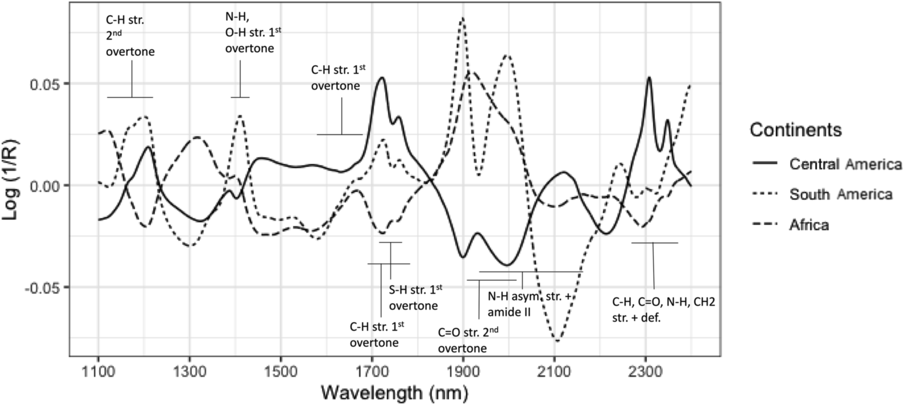

Qualifying the raw spectral data

After visual inspection of the raw spectra, preprocessing using EMSC and mean centering was applied for scatter correction. Unsupervised PCA was used for outlier detection and initial exploration. Overall, no outliers were detected and a good precision was observed among the replicates. Next, supervised classification models were then employed on the dataset, and the model classification and quality were further accessed using accuracy and a dummy classifier.

Linear partial least squares-discriminant analysis classification model

The classical and linear partial least squares-discriminant analysis (PLS-DA) was applied to understand the origin classification performance of NIR spectra at different scales, from the continental to the country and up to the regional level. At the continental level, five latent variables (LVs) were selected as optimum based on cross-validation, and explained 93.60 % and 38.80 % of X and Y variances, respectively (see Figure 2). There is no clear separation between the continents on LV1. On LV2, Africa was partially differentiated from the South American samples. There is a relatively good prediction balanced accuracy (Acc) of 0.77 which was more than the no information rate (NR) (p-value <0.05) at the continental level. It is evident from Figure 2 that there are high variations within each continent, indicating the potential country and/or regional level differences. To better investigate these variations, independent PLS-DA models were built for each continent.

Figure 2.

Partial least squares-discriminant analysis (PLS-DA) 3D scores plots at the continental level (Africa, Central America, South America).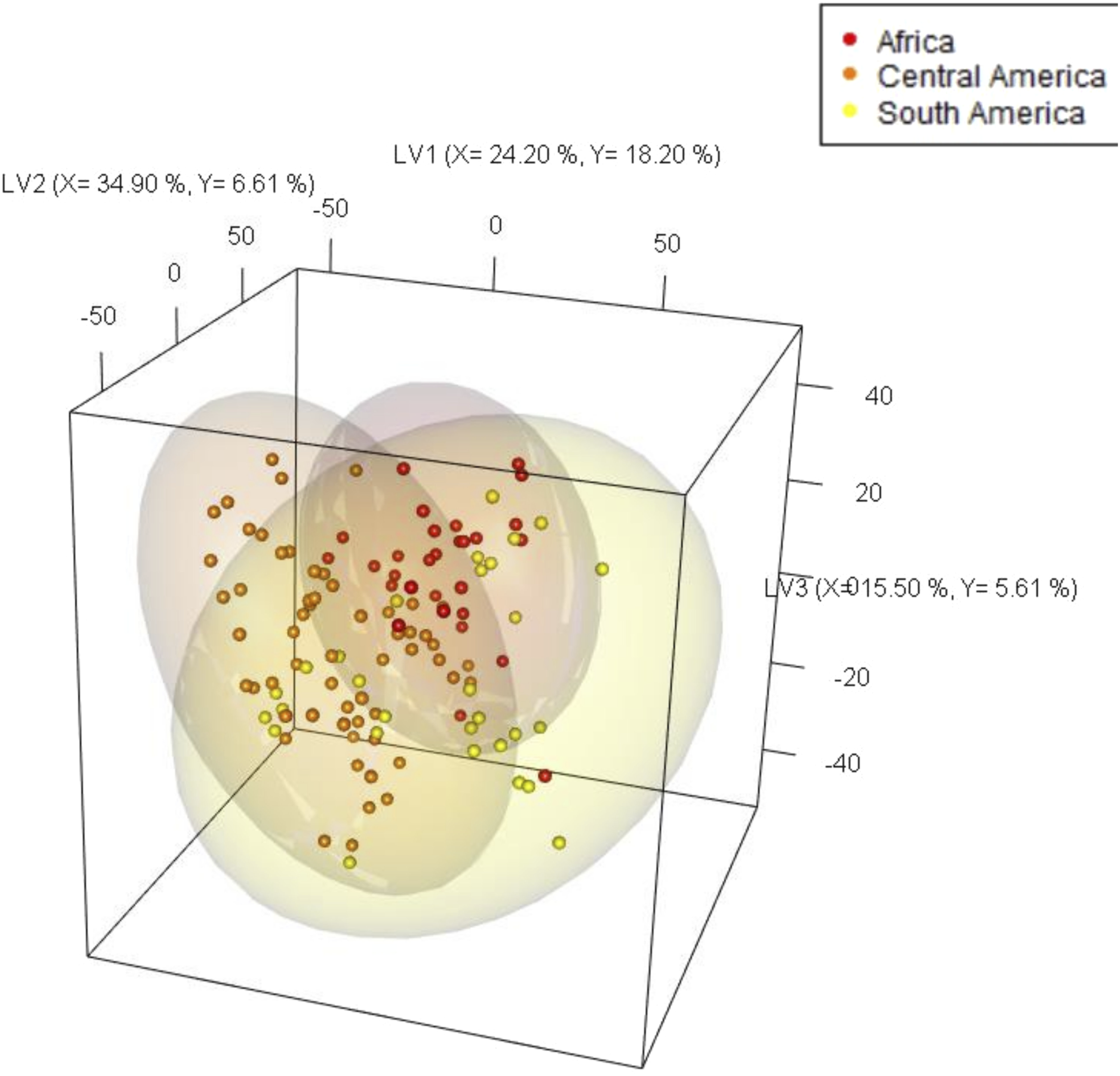

The African samples were explored using PLS-DA with Ethiopia and Kenya as the two classes (Y-variables) (Figure 3a). The model explained 87.20 % and 93.80 % of the X and Y variances, respectively. The two African country samples were differentiated on LV1, with Ethiopian coffee samples positioned on the negative loading and Kenyan samples on the positive loading. There were also variations observed within each country on LV2. The distribution of scores to spectral features can be understood through the loading weights plot, which indicates the wavelength regions important for origin discrimination from each LV. Loading weights for LV1 (Figure 3bi), have the highest contribution from carbohydrates at about 1500-1650 nm, and 2250 nm on the positive loading, cellulose at 1780 nm and the water peaks on the negative loading at around 1430 nm and 1900 nm. These results indicate that Kenyan samples could have higher carbohydrate and cellulose contents, while Ethiopian samples could contain higher levels of water. There might also be differences in the water holding capacity of the beans from the two countries. Further studies are warranted since the samples were prepared and stored the same way to control for moisture. The LV2 loading weights (Figure 3bii) show a dominance of cellulose on the positive loading at around 2080 nm, and negative loadings of proteins at around 1550 nm. These components may help explain the variations observed within each country. All the samples were predicted accurately at the country level (Acc = 1 > NR) (p-value <0.05).

Figure 3.

Partial least squares-discriminant analysis (PLS-DA) (a) 3D scores plots for Africa at the country level, (b) loading weights plot for (i) LV1, and (ii) LV2.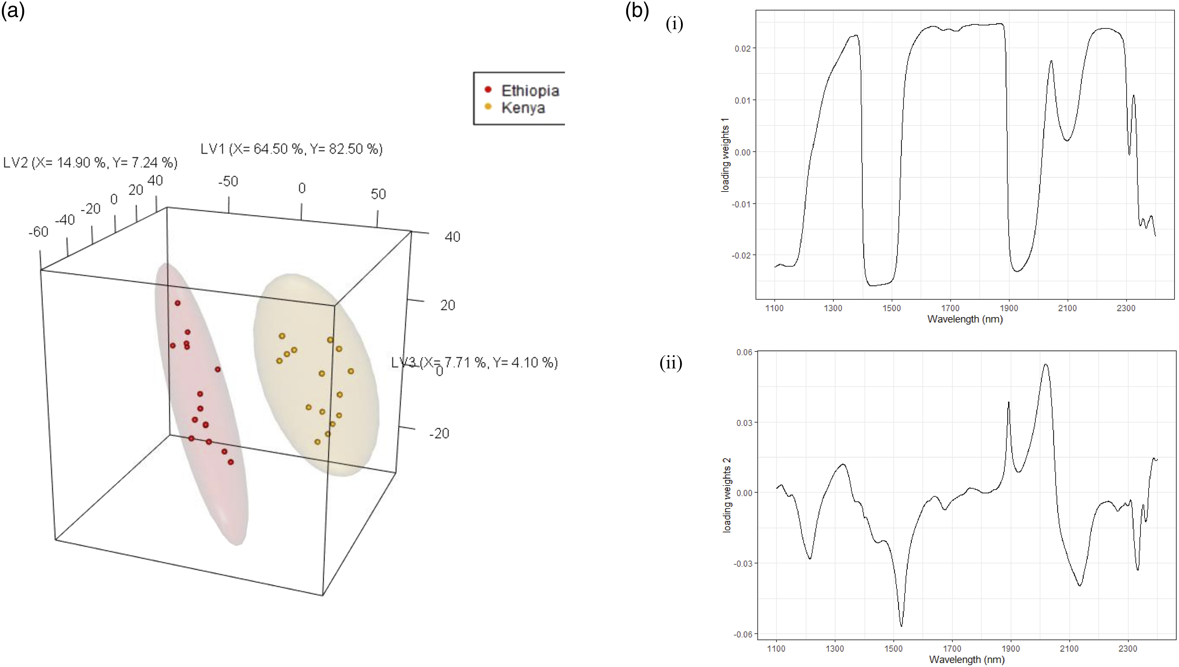

Figure 3 shows an apparent variation (mainly represented by LV3) within each African country. To investigate these variations, and to test the sensitivity of NIR with PLS-DA to classify at the regional level, the African samples were modelled using the five regions as the Y-variables. The model explained 98.50 % and 84.80 % of the X and Y variances, respectively. The Ethiopian regions (Gedio and Guji) were grouped on the positive loading of LV1, separated from the Kenyan samples (Kiajibbi, Maywal, and Yara), which were positioned on the negative loading. Loading weights for LV1 (Figure 4b) show similar results as the loading weights for LV1 for the country level model, but flipped. Water was dominant on the positive loading at around 1900 nm, with Ethiopian regional samples showing higher levels of water. Carbohydrates and cellulose again show dominance in the Kenyan regional samples. LV1 also differentiated Kiajibbi from the other Kenyan samples. Within each country, there were overlaps with Gedio and Guji from Ethiopia, and Maywal with Yara on LV1. These overlapped regions were differentiated on LV2, which showed a dominance of proteins, cellulose, and carbohydrates on the positive loading at around 2100 nm. The predictive accuracy for the African samples at the regional level was Acc of 1 > NR (p-value <0.05). This is the first study on the origin classification of African arabica coffee. Previous research on Ugandan robusta coffee showed poor differentiation from other regions.⁹

Figure 4.

Partial least squares-discriminant analysis (PLS-DA) (a) 3D scores plots for Africa at regional level, (b) loading weights plot for (i) LV1, and (ii) LV2.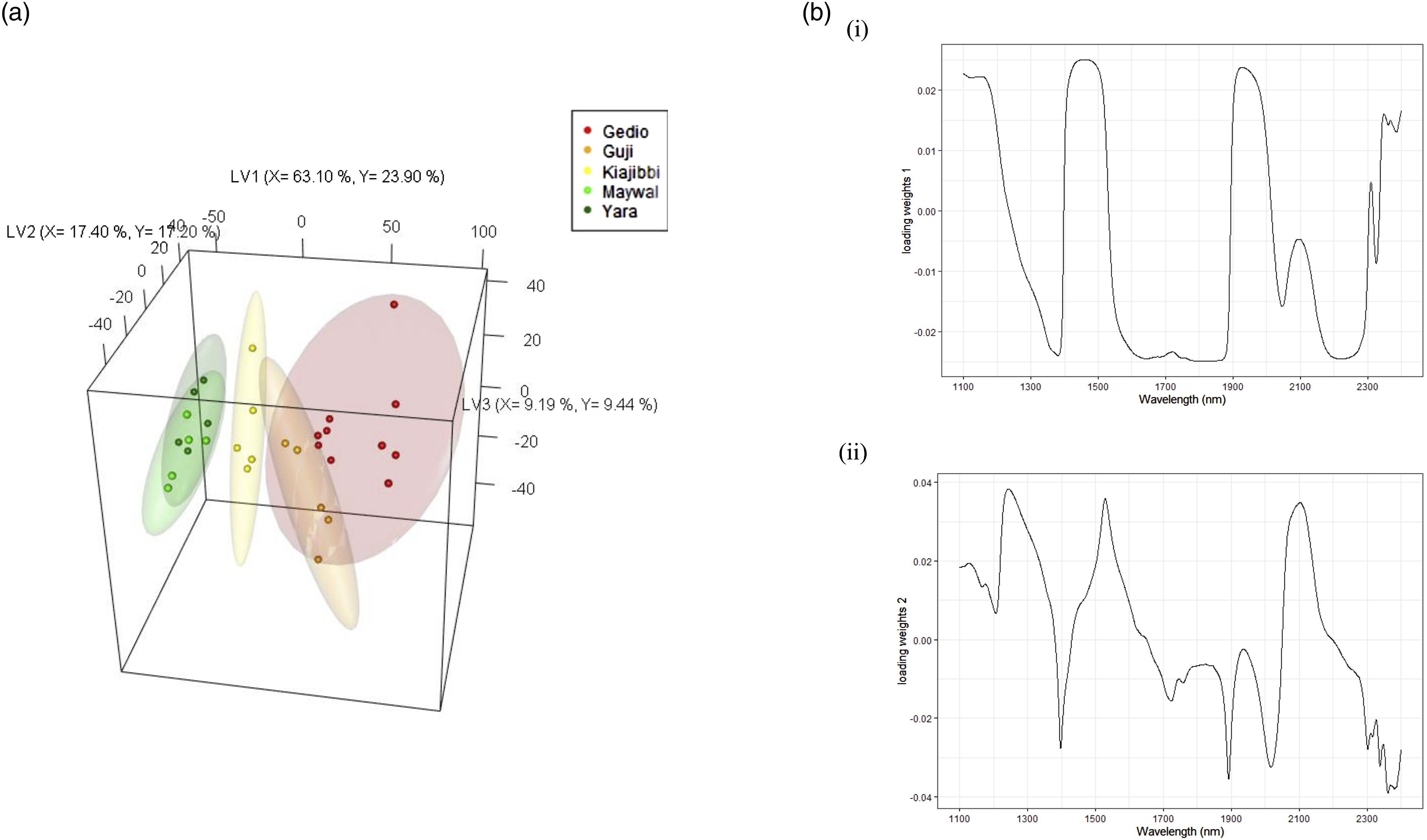

The South American samples were then modelled to study country level differences. The model explained 86.40 % and 88.10 % of the X and Y variances, respectively. The two country samples were differentiated on LV1, with Colombian samples on the negative loading and Peruvian samples on the positive loading (see Figure 5a). The loading weights in Figure 5bi show a dominance of proteins, cellulose, and carbohydrates on the positive loading and water on the negative loading. Colombian samples were characterised by lower levels of carbohydrates and proteins, while Peruvian samples had high water contents. On LV2 and LV3, differences are observed within each country, especially for samples from Colombia. The Loading weights for LV2 in Figure 5bii show a dominance of lignin and cellulose at 1700 nm and 2300 nm peaks associated with caffeine and esters.³¹ The loading weights for LV3 (Figure 5biii) showed a dominance of peaks at 2300 nm on the positive loading. All the samples were predicted accurately at the country level with Acc = 1 > NR (p-value <.05).

Figure 5.

Partial least squares-discriminant analysis (PLS-DA) (a) 3D scores plots for South America at the country level, (b) loading weights plot for (i) LV1, and (ii) LV2, (iii) LV3.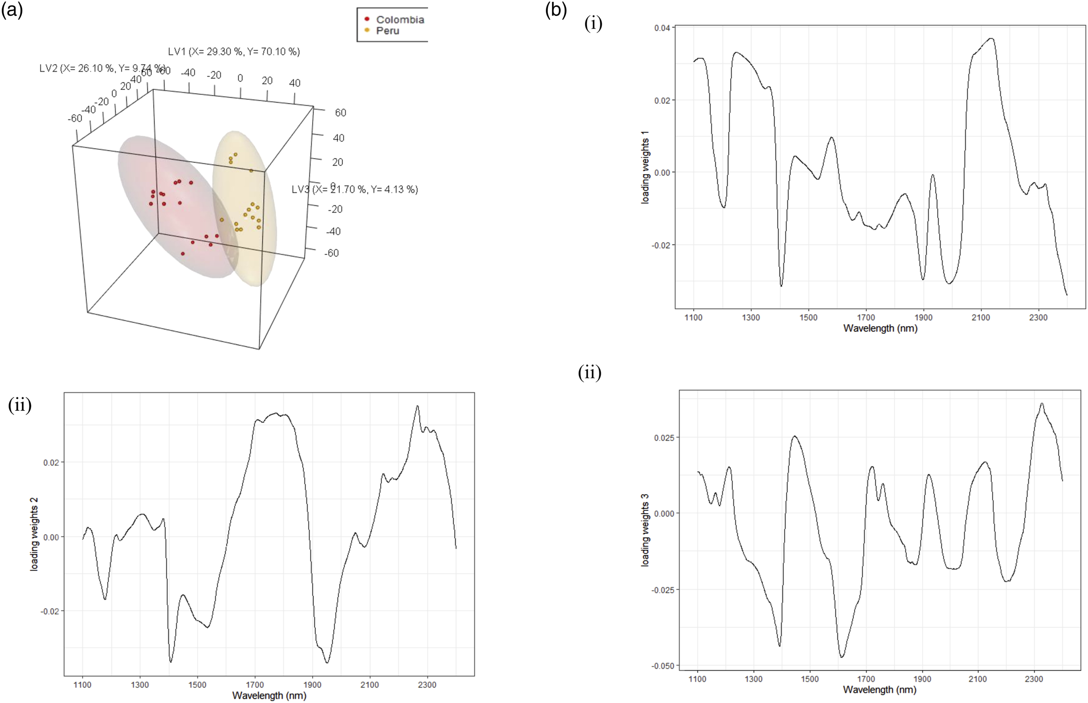

To understand regional differences within country samples on LV2 and LV3 in Figure 5, the PLS-DA model was constructed with the five South American regions as the Y- variable. The model explained 96.60 % and 77.00 % of the X and Y variances, respectively. On LV1, the Colombian (Antioquia, Huila, and Narino) regional samples were grouped on the negative loading and separated from the Peruvian (Cusco and Pasco) samples, which were grouped on the positive loading (see Figure 6a). The loading weights for LV1 (Figure 6bi) show a dominance of carbohydrates on the positive loading at 1500 nm, with Peruvian samples having higher carbohydrate contents, and Narino in Colombia having the lowest levels. These loading weights follow the similar trend as the country level model. On LV2 and LV3, regional separation was observed for both countries. The loading weights for LV2 show a dominance of carbohydrates in the positive loading, and proteins on the negative loading. The loading weights for LV3 show a dominance of cellulose on the positive loading and esters on the negative loading. The South American model also performed well at the regional level with an Acc = 1 > NR (p-value <0.05).

Figure 6.

Partial least squares-discriminant analysis (PLS-DA) (a) 3D scores plots for South America at regional level, (b) loading weights plot for (i) LV1, (ii) LV2, and (iii) LV3.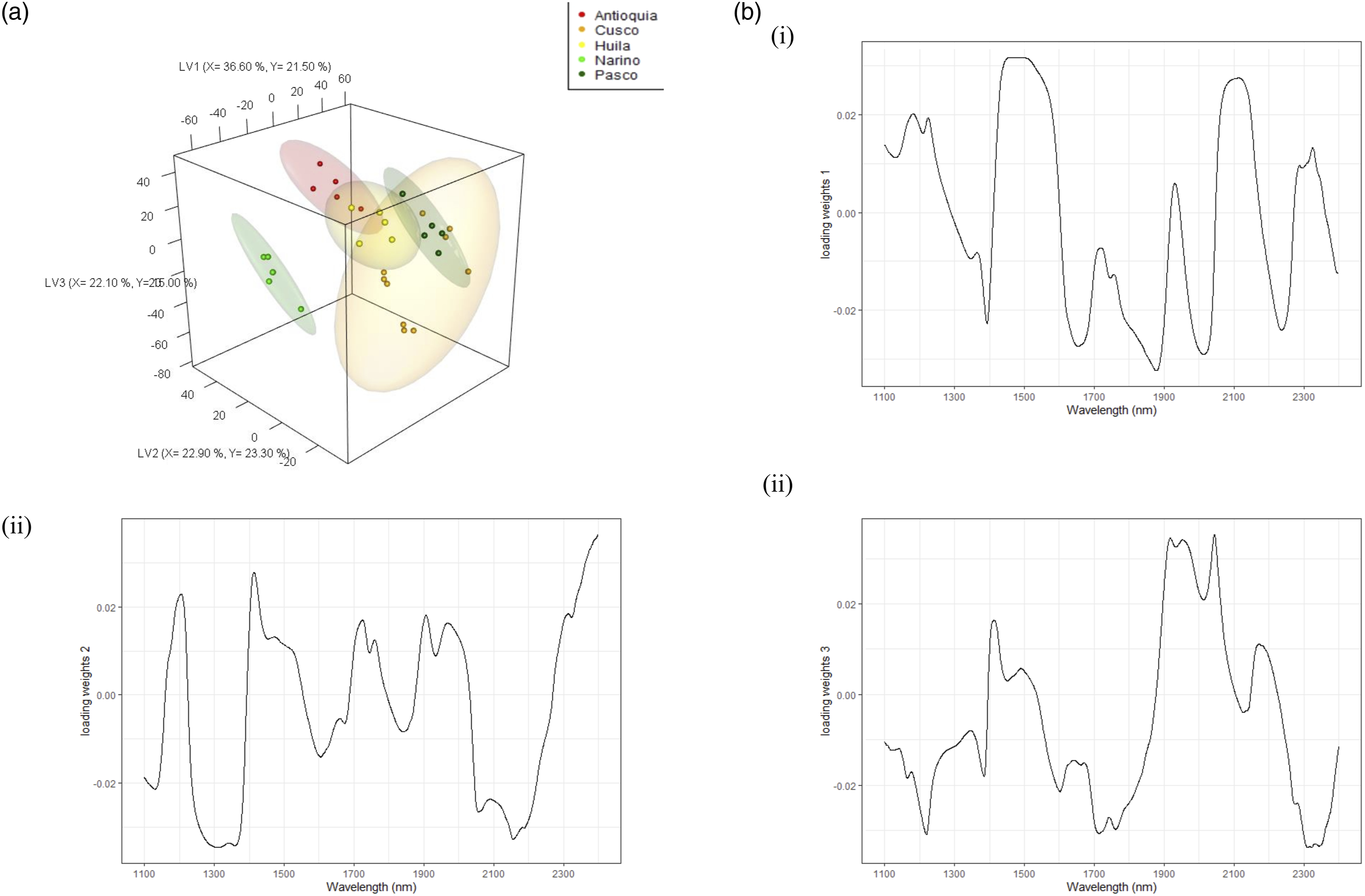

For the Central American samples, PLS-DA was employed on the four countries (Costa Rica, Guatemala, Mexico, and Nicaragua) to investigate country level differences. On LV1, Nicaragua was partially separated on the negative loading, with overlaps of the other three countries on the positive loading (see Figure 7a). The loading weights 1 (Figure 7b) show a dominance of positive loadings of lignin and cellulose around 1700 nm, and esters and caffeine around 2300 nm. These suggest that Nicaraguan samples are lower in lignin, cellulose and esters, and some regional samples in Costa Rica and Mexico have the highest amounts of these constituents.

Figure 7.

Partial least squares-discriminant analysis (PLS-DA) (a) 3D scores plots for Central America at the country level, (b) loading weights plot for (i) LV1, (ii) LV2.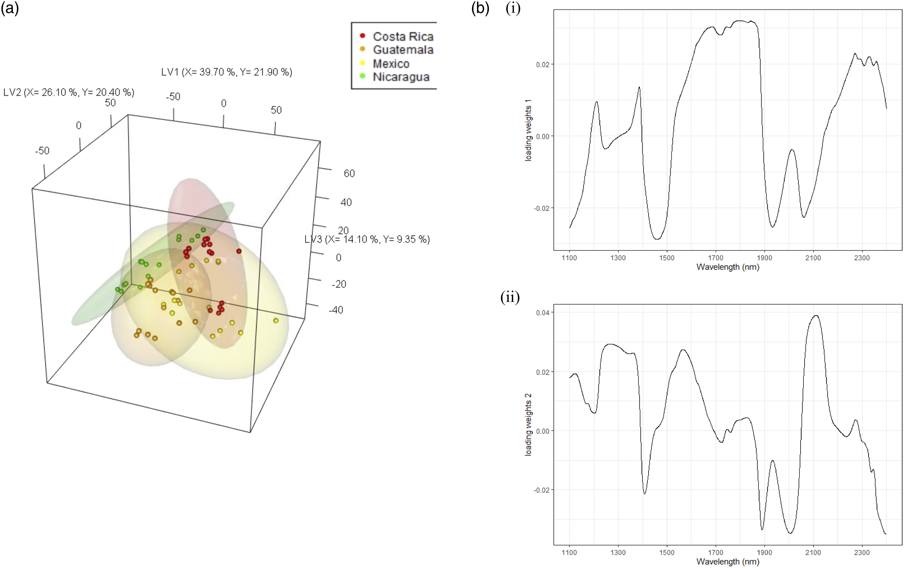

On LV2, Nicaragua and Costa Rica were partially differentiated. The loading weights (LV2) show a dominance of water on the negative loading and carbohydrates and proteins on the positive loading. Nicaraguan samples have the highest water contents, with Costa Rican samples differentiated by their higher carbohydrate and protein contents. The Central American model performed relatively well with an Acc = 0.83 > NR (p-value <0.05) at the country level.

To understand the regional differences observed in Figure 7, the model was built with the 12 regions as the Y- variable. There was no clear separation of regional samples. The predictive accuracy of the regional samples for Central America was poor at an Acc of 0.25 > NR (p-value <0.05).⁵

In summary, NIR showed sensitivity for continental classification. The variations observed within each continent were modelled to identify discriminant wavelengths for country and regional level models. The African and South American samples were most easily differentiated, with the Central American samples performing well at the country level, and poorly at the regional level. Overall, the linear PLS-DA model appeared to struggle at the Central American regional level. Non-linear machine learning modelling techniques were subsequently investigated across all origin scales to determine if classification improvement was possible even for well performing models.

Non-linear machine learning classification models

The performance of non-linear models, such as KNN, SVM, extreme gradient boost (XGB), and random forest (RF), were compared to the linear PLS-DA model. The accuracy of the training (train), cross-validation (CV) and test sets at all origin scales (continental, country, regional) without subsetting across continents are shown in Table 1.

Table 1.

Accuracy for the train, cross-validation (cv), and test set for NIR spectral datasets across the origin scales (continental. Country, regional) using five different modelling techniques [partial least squares-discriminant analysis (PLS-DA), k-nearest neighbours (KNN), support vector machine (SVM), extreme gradient boost (XGB), random forest (RF)].

Origin scale	PLS-DA				KNN				SVM				XGB				RF
Origin scale	Parameter	Train	cv	Test	Parameter	Train	cv	Test	Parameter	Train	cv	Test	Parameter	Train	cv	Test	Parameter	Train	cv	Test
Continent	5 LVs, RMSEE (0.37), R2X (0.97), R2Y (0.39), Q2 (0.30)	0.8	0.67	0.77	k = 2	0.85	0.85	0.85	Cost (10), gamma (0.01), sigma (0.00044), support_v (116)	0.75	0.95	0.68	max_depth (3), eta (0.1), ntree_limit (65), nfeatures (2701), niter (75)	0.92	0.9	0.89	mtry (52), ntree (65), oob (9.48 %)	1	0.93	0.99
Country	4 LVs, RMSEE (0.29), R2X (0.91), R2Y (0.27), Q2 (0.24)	0.6	0.53	0.58	k = 5	0.89	0.78	0.86	Cost (10), gamma (0.01), sigma (0.00049), support_v (120)	0.88	0.95	0.84	max_depth (8), eta (0.1), ntree_limit (100), nfeatures (2701), niter (100)	0.82	0.81	0.79	mtry (52), ntree (100), oob (12.50 %)	0.92	0.86	0.88
Region	4 LVs, RMSEE (0.19), R2X (0.91), R2Y (0.16), Q2 (0.13)	0.25	0.23	0.5	k = 7	0.79	0.76	0.77	Cost (10), gamma (0.01), sigma (0.00053), support_v (118)	0.58	0.83	0.46	max_depth (22), eta (0.1), ntree_limit (83), nfeatures (2701), niter (93)	0.82	0.83	0.75	mtry (52), ntree (90), oob (4.17 %)	0.94	0.94	0.88

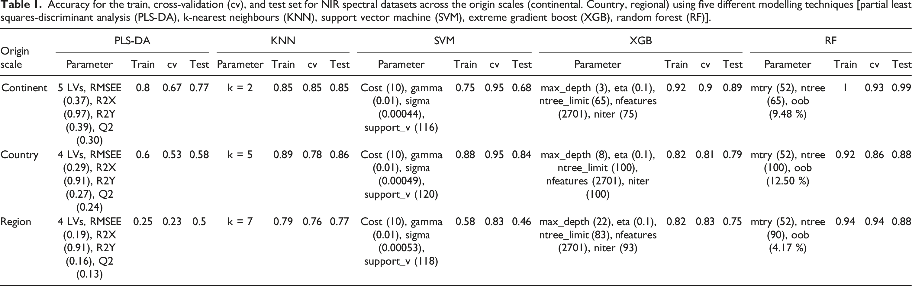
In Table 1, the continental level classification using PLS-DA achieved a relatively good performance with an Acc of 0.77. Non-linear models KNN, SVM, XGB, and RF all appeared to improve the model performance further, with the best model performance from XGB and RF, the two ensemble decision trees. At the country level, with all 8 countries set as Y, the performance was poor at an Acc of 0.58. Non-linear models increased the performance to a moderate Acc of 0.76 (KNN) and 0. 74 (SVM), and up to a good performance of 0.79 (XGB) and 0.88 (RF). Lastly at the regional level with all 22 regions in the model, the model predicted at a level of chance with poor performance even across the training and cv sets. Non-linear models again improved the performance, with XGB and RF consistently performing the best with an improved Acc of 0.80 and 0.88 respectively.

Overall, all the non-linear models have demonstrated potential in dealing with more complicated NIR spectral datasets. The results comparing the best non-linear model agree with a previous study. A bioinformatic classification study comparing 13 machine learning models also found RF and XGB to be exceptional in contrast to SVM and KNN.³⁵

Non-linear models, however, tend to be black boxes in which the innerworkings of the model is not well understood, and variable identification is lacking. While XGB appears to perform well, the mechanisms for classification are not well understood. RF on the other hand includes a built-in feature selection parameter called the Gini impurity which decides the feature (wavelength) that is more important- based on how well the decision tree was split. The features that are more important towards the prediction model show a larger mean decrease in Gini impurity. In addition, the interpretability and graphical visualisation of machine learning algorithms are important for researchers to understand predictive models qualitatively.³⁶ A proximity matrix can be calculated in RF to build a MDS (multidimensional scaling) plot - a visual representation of class similarities via a scatter plot. Proximity is the proportion of time that two classes end up in the same tree node out of all the trees in the forest.

As discussed in the previous section, the Central American regional model had a higher classification challenge with more countries sampled compared to the African and the South American model. This led to the poor predictive Acc of 0.25. Mexico is a large country by land area. This may have led to the overlap of macro and micro climates across regions, resulting in a broad range of constituent concentrations in the coffee bean.^37–41 The Central American regional dataset was thus used as an example to demonstrate the potential of non-linear RF, to see if improvements could be made to the performance, and to identify RF selected features compared to the loading weights from the linear PLS-DA model (Figure 8b).

Figure 8.

Partial least squares-discriminant analysis (PLS-DA) (a) 3D scores plots for Central America at regional level, (b) loading weights plot for (i) LV1, and (ii) LV2.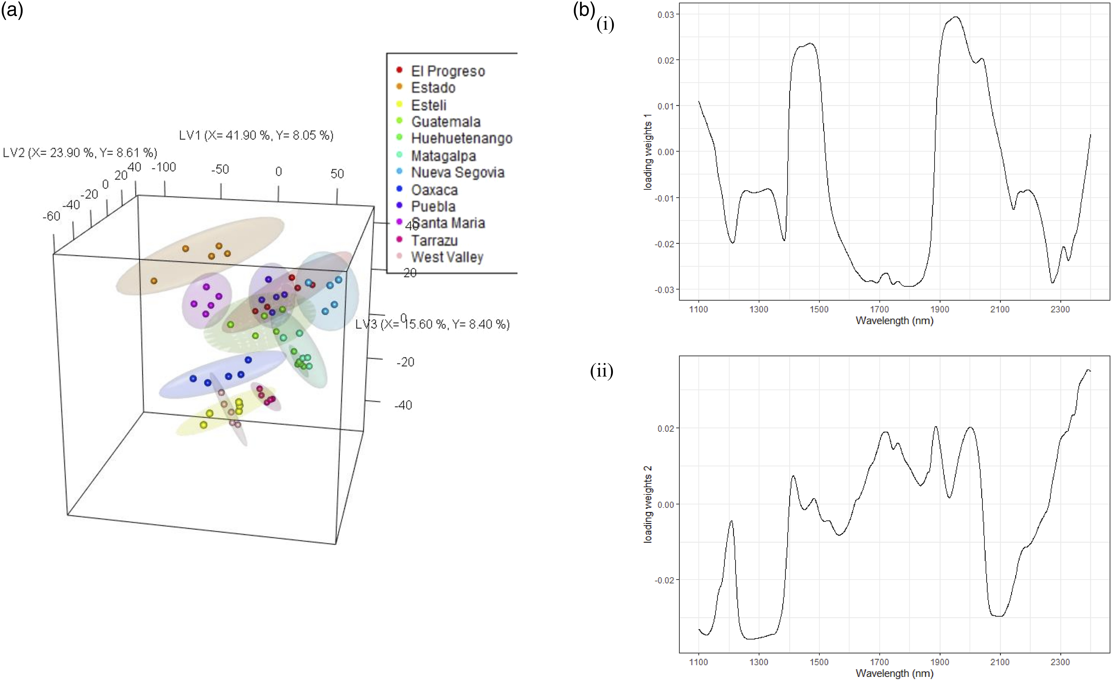

The RF MDS plot and feature selection plots in Figure 9 show some improvements visually – the regions are more distinguished. The RF feature selection plot (Figure 9b) demonstrate the wavelengths most important towards reducing the Gini impurity and thus overall model accuracy. Modelling the Central American data at regional level led to a significant increase in Acc to 0.98.

Figure 9.

Random forest (RF) (a) MDS (multi-dimensional scaling) plot, and (b) feature selection plot with the most important wavelengths indicated the Central American regional model.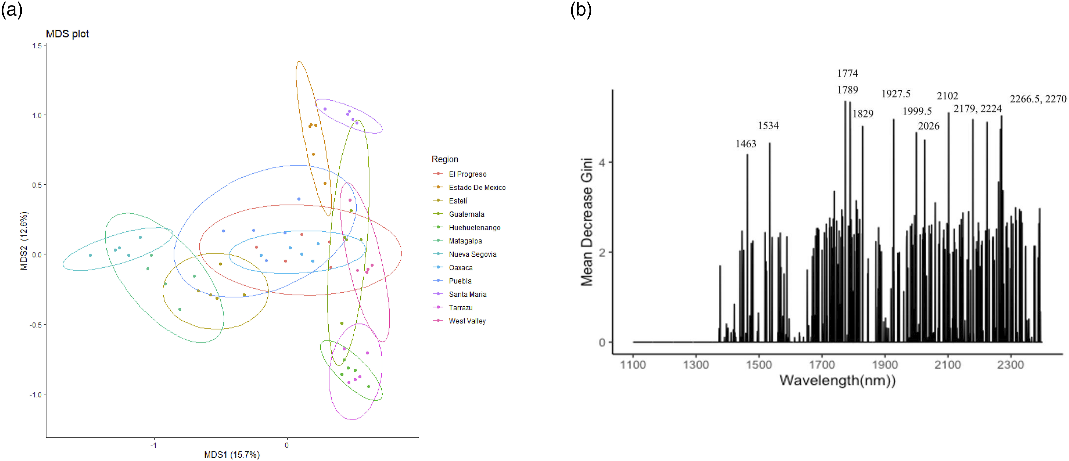

However, the visualisation (Figure 9a) does not appear to be an accurate representation of the excellent performance by the RF model given that there were overlaps across classes. To circumvent this limitation, there is growing interest in Explainable Artificial Intelligence (XAI) which aims to reveal the inner workings and mechanisms behind these complex models.⁴² More effort is needed to make machine learning models more understandable to increase transparency and veracity of predictions.

A broader range of feature selected wavelengths can be observed from the Central American regional RF model (Figure 9b). The RF selected top wavelengths were similar to the ones identified in the linear PLS-DA loading weights (see Figure 8b). Minor peaks appear to become more important when using non-linear RF machine learning models.

Conclusions

The present work demonstrated the potential of NIR spectroscopy coupled with machine learning for rapid and cost-effective origin classification of coffee from the continental to the regional level. NIR spectroscopy coupled with PLS-DA appears to be sensitive at the continent and country level, with promise at the regional level. Overall, this study is the first to indicate the potential of a variety of non-linear machine learning models to improve model performance for authentication of coffee origin. The non-linear models can better deal with complicated classification challenges compared to the linear PLS-DA model. Random forest was found to be superior to other non-linear models for their added visual illustration of the underlying discriminatory mechanisms and variable identification opportunity. Additional effort needs to be put in to enable machine learning models to be more interpretable. However, the choice of an appropriate model depends on the classification problem at hand, and for more straightforward problems, the linear models appear good enough for their simplicity. This is a preliminary study which serves as a proof of a concept demonstrating the potential of NIR spectroscopy coupled with machine learning. Each location was represented by a small number of samples, future studies will require an extended sample set with precise geographical metadata to ensure more representative sampling. The model can be extended and made robust with external validation and by considering natural variations with samples from different years, seasons, batches, and genetics. Targeted analyses can be performed to confirm the identification of the discriminative wavelength regions. There is potential for NIR spectroscopy coupled with machine learning to monitor the authenticity of coffee beans of labelled origins on a global scale, and to expand it to the verification of bean species.

Footnotes

Acknowledgements

We would like to acknowledge Oritain Global Limited for providing the green coffee bean samples, equipment, and metadata.

Declaration of conflicting interests

The author(s) declared no potential conflicts of interest with respect to the research, authorship, and/or publication of this article.

Funding

The author(s) received no financial support for the research, authorship, and/or publication of this article.

ORCID iD

Joy Sim

References

Pandiselvam

Prithviraj

Manikantan

, et al. Recent advancements in NIR spectroscopy for assessing the quality and safety of horticultural products: a comprehensive review. Front Nutr 2022; 9: 973457. DOI: 10.3389/fnut.2022.973457.

Manning

. Food fraud: policy and food chain. Curr Opin Food Sci 2016; 10: 16–21. DOI: 10.1016/j.cofs.2016.07.001.

Barbin

Felicio

ALSM

Sun

D-W

, et al. Application of infrared spectral techniques on quality and compositional attributes of coffee: an overview. Food Res Int 2014; 61: 23–32. DOI: 10.1016/j.foodres.2014.01.005.

Scholz

MBS

Pagiatto

Kitzberger

CSG

, et al. Validation of near-infrared spectroscopy for the quantification of cafestol and kahweol in green coffee. Food Res Int 2014; 61: 176–182. DOI: 10.1016/j.foodres.2013.12.008.

Marquetti

Link

Lemes

ALG

, et al. Partial least square with discriminant analysis and near infrared spectroscopy for evaluation of geographic and genotypic origin of arabica coffee. Comput Electron Agric 2016; 121: 313–319. DOI: 10.1016/j.compag.2015.12.018.

Monteiro

Santos

Alvarenga Brizola

, et al. Comparison between proton transfer reaction mass spectrometry and near infrared spectroscopy for the authentication of Brazilian coffee: a preliminary chemometric study. Food Control 2018; 91: 276–283. DOI: 10.1016/j.foodcont.2018.04.009.

Bona

Marquetti

Link

, et al. Support vector machines in tandem with infrared spectroscopy for geographical classification of green arabica coffee. LWT - Food Sci Technol (Lebensmittel-Wissenschaft -Technol) 2017; 76: 330–336. DOI: 10.1016/j.lwt.2016.04.048.

Suhandy

Yulia

Kuroki

, et al. The use of SIMCA Method and NIR spectroscopy with hand-held spectrometers equipped with integrating sphere for classification of two different Indonesian specialty coffees. J Phys : Conf Ser 2021; 1751: 012080. DOI: 10.1088/1742-6596/1751/1/012080.

Medina

Caro Rodríguez

Arana

, et al. Comparison of attenuated total reflectance mid-infrared, near infrared, and ¹H-nuclear magnetic resonance spectroscopies for the determination of coffee’s geographical origin. Int J Anal Chem 2017; 2017: 7210463. DOI: 10.1155/2017/7210463.

10.

Giraudo

Grassi

Savorani

, et al. Determination of the geographical origin of green coffee beans using NIR spectroscopy and multivariate data analysis. Food Control 2019; 99: 137–145. DOI: 10.1016/j.foodcont.2018.12.033.

11.

Wang

Bouzembrak

Lansink

, et al. Application of machine learning to the monitoring and prediction of food safety: a review. Compr Rev Food Sci Food Saf 2022; 21: 416-434. DOI: 10.1111/1541-4337.12868.

12.

Zareef

Chen

Hassan

, et al. An overview on the applications of typical non-linear algorithms coupled with NIR spectroscopy in food analysis. Food Eng Rev 2020; 12: 173–190. DOI: 10.1007/s12393-020-09210-7.

13.

R Core Team . R: a language and environment for statistical computing. Vienna, Austria: R Foundation for Statistical Computing, 2022.

14.

Afseth

Kohler

. Extended multiplicative signal correction in vibrational spectroscopy, a tutorial. Chemometr Intell Lab Syst 2012; 117: 92–99. DOI: 10.1016/j.chemolab.2012.03.004.

15.

Martens

Stark

. Extended multiplicative signal correction and spectral interference subtraction: New preprocessing methods for near infrared spectroscopy. J Pharm Biomed Anal 1991; 9: 625-635. DOI: 10.1016/0731-7085(91)80188-f.

16.

Kuhn

. Building predictive models in R using the caret package. J Stat Softw 2008; 28: 1–26. DOI: 10.18637/jss.v028.i05.

17.

Wei

Dunbrack

Jr . The role of balanced training and testing data sets for binary classifiers in bioinformatics. PLoS One 2013; 8: e67863. DOI: 10.1371/journal.pone.0067863.

18.

Brodersen

Ong

Stephan

, et al. The balanced accuracy and its posterior distribu+tion. In: 2010 20th International Conference on Pattern Recognition, Istanbul, Turkey, 23-26 August 2010, pp. 3121–3124.

19.

Ballabio

Consonni

. Classification tools in chemistry. Part 1: linear models. PLS-DA. Anal Methods 2013; 5: 3790. DOI: 10.1039/c3ay40582f.

20.

Thévenot

Roux

, et al. Analysis of the human adult urinary metabolome variations with age, body mass index, and gender by implementing a comprehensive workflow for univariate and oPLS statistical analyses. J Proteome Res 2015; 14: 3322–3335. DOI: 10.1021/acs.jproteome.5b00354.

21.

Aliakbarzadeh

Parastar

Sereshti

. Classification of gas chromatographic fingerprints of saffron using partial least squares discriminant analysis together with different variable selection methods. Chemometr Intell Lab Syst 2016; 158: 165–173. DOI: 10.1016/j.chemolab.2016.09.002.

22.

Šašić

Ozaki

. Short-wave near-infrared spectroscopy of biological fluids. 1. Quantitative analysis of fat, protein, and lactose in raw milk by partial least-squares regression and band assignment. Anal Chem 2001; 73: 64–71. DOI: 10.1021/ac000469c.

23.

Guo

Wang

Bell

, et al. KNN model-based approach in classification. OTM Confederated International Conferences” On the Move to Meaningful Internet Systems 2003; 1: 986–996. DOI: 10.1007/978-3-540-39964-3_62.

24.

Zhang

. Introduction to machine learning: k-nearest neighbors. Ann Transl Med 2016; 4: 218. DOI: 10.21037/atm.2016.03.37.

25.

Hearst

Dumais

Osuna

, et al. Support vector machines. IEEE Intell Syst Their Appl 1998; 13: 18–28. DOI: 10.1109/5254.708428.

26.

Jarvis

Goodacre

. Genetic algorithm optimization for pre-processing and variable selection of spectroscopic data. Bioinformatics 2005; 21: 860-868. DOI: 10.1093/bioinformatics/bti102.

27.

Meyer

Dimitriadou

Hornik

, et al. e1071: misc functions of the department of statistics, probability theory group formerly: E1071). R Cran: TU Wien, 2023.

28.

Quinlan

. Learning decision tree classifiers. ACM Comput Surv 1996; 28: 71–72. DOI: 10.1145/234313.234346.

29.

Menze

Kelm

Masuch

, et al. A comparison of random forest and its Gini importance with standard chemometric methods for the feature selection and classification of spectral data. BMC Bioinf 2009; 10: 213–216. DOI: 10.1186/1471-2105-10-213.

30.

Torgerson

. Multidimensional scaling: I. Theory and method. Psychometrika 1952; 17: 401–419.

31.

Buratti

Sinelli

Bertone

, et al. Discrimination between washed arabica, natural arabica and robusta coffees by using near infrared spectroscopy, electronic nose, and electronic tongue analysis. J Sci Food Agric 2015; 95: 2192-2200. DOI: 10.1002/jsfa.6933.

32.

Ribeiro

Ferreira

MMC

Salva

TJG

. Chemometric models for the quantitative descriptive sensory analysis of arabica coffee beverages using near infrared spectroscopy. Talanta 2011; 83: 1352-1358. DOI: 10.1016/j.talanta.2010.11.001.

33.

Czarnecki

Beć

Grabska

, et al. Overview of application of nir spectroscopy to physical chemistry. In: Ozaki

Huck

Tsuchikawa

, (eds). Near-infrared spectroscopy: theory, spectral analysis, instrumentation, and applications. Singapore: Springer Singapore, 2021, pp. 297–330.

34.

Grabska

Beć

Ozaki

, et al. Anharmonic DFT Study of near-infrared spectra of caffeine: vibrational analysis of the second overtones and ternary combinations. Molecules 2021; 26: 5212. DOI: 10.3390/molecules26175212.

35.

Olson

Cava

Mustahsan

, et al. Data-driven advice for applying machine learning to bioinformatics problems. Pac Symp Biocomput 2018; 23: 192–203. DOI: 10.48550/arXiv.1708.05070.

36.

Ribeiro

Singh

Guestrin

. “Why should i trust you?” Explaining the predictions of any classifier. In: Proceedings of the 22nd ACM SIGKDD international conference on knowledge discovery and data mining, San Francisco, USA, 13-17 August 2016, pp. 1135–1144. DOI: 10.48550/arXiv.1602.04938.

37.

Bertrand

Boulanger

Dussert

, et al. Climatic factors directly impact the volatile organic compound fingerprint in green arabica coffee bean as well as coffee beverage quality. Food Chem 2012; 135: 2575–2583. DOI: 10.1016/j.foodchem.2012.06.060.

38.

Joët

Laffargue

Descroix

, et al. Influence of environmental factors, wet processing and their interactions on the biochemical composition of green arabica coffee beans. Food Chem 2010; 118: 693–701. DOI: 10.1016/j.foodchem.2009.05.048.

39.

Joet

Bertrand

Dussert

. Environmental effects on coffee seed biochemical composition and quality attributes: a genomic perspective. In: 25th International Scientific Colloquium on Coffee, 08-13 September 2014, Colombia.

40.

Teuber

. Geographical indications of origin as a tool of product differentiation: the case of coffee. J Int Food & Agribus Mark 2010; 22: 277–298. DOI: 10.1080/08974431003641612.

41.

Worku

De Meulenaer

Duchateau

, et al. Effect of altitude on biochemical composition and quality of green arabica coffee beans can be affected by shade and postharvest processing method. Food Res Int 2018; 105: 278-285. DOI: 10.1016/j.foodres.2017.11.016.

42.

Buyuktepe

Catal

Kar

, et al. Food fraud detection using explainable artificial intelligence. Expet Syst 2023; 2023: e13387. DOI: 10.1111/exsy.13387.