Sage Journals: Discover world-class research

Abstract

Near infrared spectroscopy is widely used to rapidly and cost-effectively collect chemical information from plant samples. Large datasets with hundreds to thousands of spectra and reference values are increasingly becoming more common as researchers accumulate data over many years or across research groups. These datasets potentially contain great spectral and chemical variation and could produce a broadly-applicable calibration model. In this study, partial least squares regression was used to model relationships between near infrared spectra and the foliar concentration of two ecologically-important chemical traits, available nitrogen and total formylated phloroglucinol compounds in Eucalyptus leaves. The nested spatial structure within the extensive dataset of spectra and reference values from 80 species of Eucalyptus was taken into account during calibration development and model validation. Geographic variation amongst samples influenced how well available nitrogen could be predicted. Predictive error of the model was greatest when tested against samples from different Australian states and local government areas to the calibration set. In addition, the results showed that simply relying on spectral variation (assessed by Mahalanobis distance) may mislead researchers into how many reference values are needed. The prediction accuracy of the model of available nitrogen differed little whether 300 or up to 987 calibration samples were included, which indicated that an excessive number of reference values were obtained. Lastly, a suitable multi-species calibration for formylated phloroglucinol compounds was produced and the difficulties associated with predicting complex chemical traits were discussed. Directing effort towards broadly applicable models will encourage sharing of calibration models across projects and research groups and facilitate the integration of near infrared spectroscopy in many research fields.

Keywords

Available nitrogen forage quality formylated phloroglucinol compounds herbivore large datasets near infrared partial least squares regression sample size

Introduction

Near infrared (NIR) spectroscopy is a non-destructive, fast and accurate technology, which is used to answer research questions in many fields. As this technology has become more readily available, large datasets are increasingly becoming more common. Accumulating spectra and reference values over many years or across projects and research groups can lead to large datasets with thousands of samples.^1–3 Large datasets (>1000 samples) that are used to predict chemical traits from near infrared spectra present particular challenges in chemometrics. As a project accumulates ever more samples with more diversity, the dataset intrinsically contains greater chemical and spectral variation that must be represented in a robust calibration model. If captured successfully, however, researchers can develop a broadly applicable “global” calibration model that encapsulates chemical diversity.⁴ Reducing time and cost for NIR calibration development would benefit many fields such as forestry, agriculture, pharmaceutics and ecology where large datasets are becoming more common. In saying that, it is still unclear how best to explore, capture and utilise the variation inherent within a large dataset.

Investing in a global calibration involves substantial initial costs, and so approaches to reduce the time and costs of model development are valuable. To tackle a large and diverse dataset, one must explore the sources of compositional variation and how it can assist in the selection of samples for calibration and validation of models. Variation originates from differences across measurement days,⁵ plant parts,⁶ plant species⁷ and laboratories.¹ Ecological studies present unique challenges because they can extend over a variety of environments, climates and plant taxonomic groups and the data are inherently more variable than those of an agricultural commodity or a pharmaceutical product.⁸ Models developed in ecological studies are usually restricted to site-specific analyses and have questionable utility for applications outside the collection sites of the calibration set.^9–15 However, there have been some successes in creating global calibration models across wide areas, which open the door to further improvements in model performance.¹⁶

Over many years, sharing of samples and NIR spectra in agricultural research groups has facilitated the compilation of very large datasets.^1,17 For example, studies have collated over 25,000 forage samples (e.g. legumes and grasses) from seven countries and compared calibration methods for moisture, crude protein and neutral detergent fibre.¹ The authors found differences in the predictive performance of the calibration equations on independent datasets and that performance could be improved with different statistical techniques and standardisation of instruments and procedures. In addition to these suggestions, taking account of nested spatial structure in large datasets would also improve the performance of global calibrations.

In this study, calibration methods for quantitative NIR spectroscopy were explored using a diverse dataset of Eucalyptus leaves. The samples were collected as part of a larger landscape study of variations in forage quality for the koala (Phascolarctos cinereus). A robust global calibration of the nutritional quality of tree leaves is important for investigations into plant-animal interactions and patterns of animal distribution and abundance,^18–20 aiding wildlife management and conservation. The choice of a large ecological dataset with samples from many origins allowed for the exploration of the influence of nested structure (structures within the data where samples can be grouped based on similar properties) and broadened the understanding of different approaches for global calibration development.

An ecological study – Eucalypt forage quality

The nutritional quality of eucalypt leaves for vertebrate herbivores has been widely studied and researchers have identified several chemical traits that contribute to foraging behaviour, habitat selection, and reproductive success in populations of wild folivores.²¹ The chemical traits that have been most useful for determining eucalypt forage quality are the foliar concentrations of available protein¹² and formylated phloroglucinol compounds (FPCs).²²

Available protein or available nitrogen (N_A, with nitrogen being a proxy for protein) is an integrative measure that accounts for the effect of tannins on the amount of total nitrogen (N_T) available for digestion. Tannins are a class of secondary compounds commonly found in many plants, which can make plant proteins unavailable to the animal. The variability of N_A in eucalypt leaves across a landscape has been shown to explain the reproductive success of the common brushtail possums (Trichosurus vulpecula) and the growth rate of their offspring,¹² as well as food tree choice by wild greater gliders (Petauroides volans)¹⁰ and koalas.¹³ In addition, N_A is an influential factor in forage quality for a number of herbivorous species outside of Australia, such as moose in Alaska²³ and spider monkeys in Bolivia.²⁴

FPCs are a diverse group of terpene adducts found largely in the eucalypt subgenus Symphyomyrtus. FPCs have unknown physiological effects in animals but their intake is strongly regulated because they cause nausea and aversions to feeding.²⁵ There are approximately 30 known FPC compounds found in different eucalypts, many as very minor components. Previous studies have focussed on quantifying approximately 17 of the most common of these²⁶ and so quantifying the total FPC concentration in eucalypt leaves is much more difficult using NIR spectra than it is for N_A. Previously, FPC calibration models have only been developed for one to three eucalypt species at a time^9–11 and fewer than 10 species have been studied.²⁶ Developing calibration models for complex chemical traits, like FPCs, across a large number of species with significant spectral and chemical diversity is not simple but is essential to facilitate landscape–scale studies of plant-animal interactions.

Calibration development and model validation

Often, cost and laboratory restrictions dictate compromises during calibration development and users must understand the consequences of these decisions. Some important considerations are how to select calibration samples, how many reference samples are required for calibration, how to validate the model, what is a realistic predictive error for independent samples, how to identify suitable/unsuitable spectra for calibration and what standardised chemical trait(s) can be used to compare taxonomically-diverse samples. In addition, there are a suite of chemometric options for developing calibration models and the suitability of these options vary depending on the application and the properties of the dataset.^27,28

Partial least squares (PLS) regression is widely used for modelling NIR data. It is a powerful multivariate technique that finds latent factors in the data to maximise the covariance between spectra and the chemical trait. To ensure that the underlying relationship is captured in a PLS model, researchers typically perform cross-validation on the calibration set. The newly developed calibration model is then tested using spectra from independent samples, the validation set, to ensure that the model is neither over-fitted nor under-fitted.^27,28 In this instance, the predicted values from the model and reference values of the independent dataset are compared. When an independent test is not available, researchers typically subdivide their reference value data into a calibration and validation set.

While it is better to have more genuinely independent samples, the nested structure within large datasets may indicate how best to split the reference value data.²⁹ Using a variety of subdivision techniques during cross-validation may provide a fairer assessment of the predictive capability of the model for future samples. Three common types of cross-validation techniques were investigated in this study:

Leave One Out (LOO_CV): one sample is put aside at each iteration.

Leave Group Out (LGO_CV): calibration samples are split into groups with similar characteristics such as geographic location.

Random subset (RS_CV): K-fold or Monte Carlo groupings: samples are randomly allocated into groups of a set size.

Using nested structure when selecting validation samples (cross-validation technique ii) is likely to provide a tougher, and therefore more convincing, test of the calibration. Introducing tougher challenges during model development should lead to a more robust global calibration which can then be applied with confidence to new samples. Further, it is widely accepted that LOO_CV (cross-validation technique i) should be used for small datasets only as it tends to select models that are over-complex. The problem is that leaving out a single observation is in general too small a perturbation to be an adequate test of the robustness of a model.

Aims

Available nitrogen: Using the nested structure

The first aim of this study was to produce a calibration model for N_A that could accommodate the variation in a multi-tree species, multi-site database and its performance was estimated on three independent datasets. The spectra of samples may be similar within groups (e.g. samples collected from a similar geographic area or across the same or closely-related species).^1,5,6 Thus, this study tested whether using nested structure during cross-validation and validation could provide a more realistic assessment of the sensitivity of the model for new samples.

Available nitrogen: How many calibration samples do you really need?

The second aim explored how the number of samples included in calibration development affected the modelled relationship between NIR spectra and N_A. Selecting samples for laboratory analysis is typically based on the variability of spectra (as indicated by metrics such as the Mahalanobis distance). However, the variation in the chemical trait of interest may not explain all of the variation in spectra.⁵ Satisfactory calibrations for N_A has been previously established,^11,14,20 and it is possible that selecting samples based on spectral variation alone may lead to an excessive number of reference value samples. This study investigated how the number of calibration samples can influence the predictive accuracy of a model by splitting the reference value data.

FPC calibration: Do you need every compound?

The third aim was to develop a single FPC calibration model using a multi-species dataset. The study investigated whether the 17 FPC compounds that have served as a relative measure of total foliar FPCs in past studies^10,30 were necessary for robust calibrations of total FPCs or whether the same accuracy could be achieved with a smaller subset of compounds. It was expected that a subset of prominent compounds could be predicted with higher accuracy, facilitating model calibration and increased prediction accuracy for total FPCs.

Methods and materials

Sample collection

All data were collected as part of a large landscape project that covered eastern and southern Australia (Figure 1). Samples sites included a variety of ecosystems such as coastal, subalpine and semi-arid Australia. Mature, fully expanded eucalypt leaf samples were collected over two field seasons; September 2012–April 2013 (field season one, 2096 samples) and September 2013–April 2014 (field season two, 1566 samples). Leaf samples were collected using a throw-line launcher.³¹ Samples were frozen immediately in dry ice and upon return to the laboratory were stored in a freezer at –20°C until they could be further processed (no longer than two months from collection).

Figure 1.

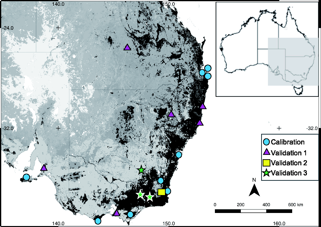
Map of study sites across four Australian states; Queensland, New South Wales, Victoria and South Australia. Land cover is represented by the shading of the map. Local government areas are marked by different shapes to represent calibration or validation samples.

Sample preparation and spectral collection

Each sample was freeze-dried and ground to pass a 0.5 mm screen using a FOSS Cyclotec 1093 cyclone mill (Foss, Hilleroed, Denmark). Ground samples were stored in sealed polyethylene containers at 22°C and away from light. For each sample, two subsamples of ground leaf powder were presented to the instrument. Spectra were collected at 2 nm intervals from 400 to 2498 nm using a scanning near infrared spectrophotometer (Foss-NIRSystems 6500; www.foss.com) with a spinning cup attachment. If the root mean squared error of the difference between the two spectra [expressed as log (1/R)/10⁶] was less than 150, the replicates were averaged. If the root mean squared error was greater than 150, the spectra were re-collected from the sample. This work was conducted in a laboratory at 18–22°C. The large eucalypt dataset was split differently to develop N_A and FPC calibration models (described in the following sections and summarised in Table 1).

Table 1.

Summary of data used for calibration model development to predict available nitrogen and formylated phloroglucinol compounds.

							Calibration				Validation
Analysis	Units	Dataset name	Subgenera	Dataset size	Reference samples	SEL	N (samples)	Range	SD	Mean	N (samples)	Range	SD	Mean
Available nitrogen	%	N_A	Monocalyptus Symphymyrtus Angophora Corymbia	2096	987	0.03	987	0.2–2.4	0.33	1.03
		Validation1	Monocalyptus Symphymyrtus		37	0.06							37	−0.02–1.81	0.40	0.74
		Validation2			11	0.08					11	−0.02–1.81	0.59	0.97
		Validation3			84	0.04					84	0.03–2.05	0.40	1.25
TotalFPCs₁₇	mg.g⁻¹	FPC	Symphymyrtus	1605	329	1	200		0–53	11	13	129	0–59	12	17
TotalFPCs₈		FPC	Symphymyrtus	1605	329	1	200	0–46	10	10	0–58	129	10	13

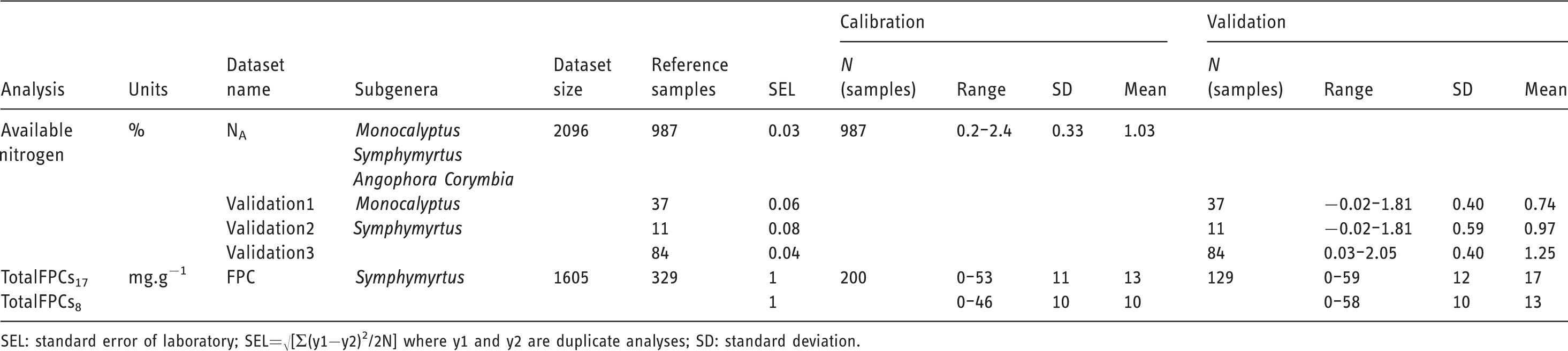
SEL: standard error of laboratory; SEL=√[Σ(y1−y2)²/2N] where y1 and y2 are duplicate analyses; SD: standard deviation.

Available nitrogen

Calibration data description and selection

The N_A calibration models were developed using field season one data only (N = 2096 samples). A subset of samples that represented the spectral variation of the dataset was identified using the CENTER and SELECT functions in the software WinISI III version 1.50E (Infrasoft International, Port Matilda, PA, USA). The CENTER algorithm ranked each spectrum based on its Mahalanobis distance (H distance) to the average spectra and the SELECT algorithm identifies a suitable calibration set for reference chemistry analyses. Using a H distance of 0.6, 987 out of 2096 samples were selected for N_A analysis and calibration development. Principal component analysis (PCA) was performed on all spectral data (N = 2096), while inspecting whether spectra clustered based on any known variables such as geographic location or species. Because sample selection based on Mahalanobis distance is highly sensitive to the presence of outliers, gross outliers were checked using plots of PC scores and of Q-residuals versus Hotelling T² (Q vs. T² plot) within-model distances. Numbers of PCs that captured approximately 90% of the spectral variance were chosen.

Spectral pretreatments

An established in vitro digestion method was used to determine N_A of each sample³² and a summary can be found in Supplementary material 1. Calibration models were developed in MATLAB R2016b. Spectra were cropped to 1102–2498 nm, Savitzy-Golay derivatives³³ were taken to eliminate an additive baseline that arose from non-relevant physical differences such as particle size and standard normal variate or multiplicative scatter correction was applied to each spectrum. Based on prior experience with these low-noise instruments, several combinations of spectral pre-treatments were tested and a summary of these are found in Supplementary material 2. The best pre-treatment for both nutritional traits (based on the most parsimonious model with the simplest math treatment) for spectra was first-derivative with a gap window of 7, second order polynomial and standard normal variate (Supplementary material 3).

Calibration development and internal validation: Using the nested structure

The samples used for chemical analysis (referred hereafter as reference value data, N = 987) were split in four ways and whether there was an ideal technique to subdivide reference value data into a calibration and a split-off validation set was investigated. The reference value data were split randomly, by sample site, by local government area (for example, Brisbane) and by Australian state (for example, New South Wales). Simultaneously, eight different cross-validation techniques against the various splits of the reference value data were compared.

Leave One Out (LOO_CV): partition one sample.

Leave Group Out (LGO_CV): partition samples based on nested geographic structure in the dataset.

SiteCode_CV: partition data by sample site (59 sample sites)

LocalArea_CV: partition data by local government area (17 local areas)

State_CV: partition data by Australian state (4 states)

Random subset (RS_CV): randomly partition reference value data into groups with a set number of samples.

RS₉₈: partition reference value data into 98 groups of 10 samples

RS₅₉: partition reference value data into 59 groups of 17 samples (SiteCode)

RS₁₇: partition reference value data into 17 groups of 61 samples (LocalArea)

RS₄: partition reference value data into 4 groups of 154 samples (State)

The robustness of the calibration models was assessed by testing the calibration model on the validation samples. The root mean squared error of cross-validation (RMSECV) of the models and root mean squared error of prediction (RMSEP) on the split-off validation samples were compared.

External validation

All reference value samples were combined into a single N_A calibration set (N = 987) to explore potential challenges for developing a robust calibration model. All eight cross-validation techniques discussed previously were performed on this combined dataset. The RMSECV curves of the calibration models and selected models with the fewest PLS factors and lowest RMSECV were compared. This informal trading-off of model complexity versus fit might be criticized as subjective, but in a situation where the validation sets are likely to be very challenging, the aim was to be more conservative in selecting numbers of factors than most formal rules would have been. These newly developed PLS models were then tested on three independent validation sets with samples from three separate projects. Three different users collected the spectra; however, all samples were scanned on the same spectrometer.

Validation1: Eucalypt leaf samples from field season two. Samples were collected in sample sites different to those in field season one.

Validation2: Eucalypt leaf samples from four sites in Tantawangalo (NSW).

Validation3: Eucalypt leaf samples collected from three sites in NSW and Victoria (Vic) for an unrelated study.

The predictive performance of the eucalypt model was tested by altering the number of PLS factors. Using all reference value samples, 30 PLS models were developed with from 1 to 30 PLS factors and the models were tested against Validation1, Validation2 and Validation3 datasets. The three resulting plots of RMSEP values were compared with the eight RMSECV curves. Samples from these validation sets were not used during calibration development.

Calibration development and validation: How many samples do you really need?

To reveal if all samples were required to best explain the relationship between NIR spectra and N_A, a series of calibration models were developed and the number of samples included during calibration were varied. Using the reference value data, 886 samples were randomly allocated to a model development set and 101 samples to a “set–aside” validation set. A series of PLS models were developed and both the number of PLS factors and number of calibration samples were varied. Using the model development set, 50 samples were selected using the SELECT function (as described earlier) and 30 models with 1–30 PLS factors were developed. These models were then tested against the split-off 836 samples and the set-aside validation set (N = 101). This step was repeated but the number of calibration samples selected were increased in increments of 50. For example, second round = selected 100 calibration samples and 786 split-off validation samples, third round = 150 calibration samples and 736 split-off validation samples. A total of 510 PLS models (17 increments, 30 PLS factors) were tested against both the split-off validation sets and the set-aside validation set (N = 101). The previous steps were then repeated; however, instead of using the WINISI SELECT function to select the various calibration sets, the calibration samples were randomly selected from the model development set.

Formylated phloroglucinol compounds

Calibration data description and selection

Samples collected across the large eucalypt dataset (N = 3662) were used to develop a multi-species, multi-site FPC calibration model. Only samples from the eucalypt subgenera Symphyomyrtus contain FPCs so the data was reduced from 3662 to 1605 samples after removing the other subgenera. To select a representative subset of samples, the CENTER and SELECT (with a H distance of 0.6) functions in WINISI III were again used and the selection of samples was constrained to a total of 400 samples for FPC analysis. Of these samples, 80 were excluded as they showed no evidence of FPCs upon analysis. Samples with zero analyte are of course informative, but the distribution of the analyte is already heavily concentrated on low values and it was desirable not to skew the calibration any further. A better solution might have been to include all the zeros and use a calibration approach that was able to cope with such analyte distributions,³⁴ but this was not tried. It was ensured that each transect (FPC dataset) and Symphyomyrtus species were represented in the reference set and samples were added when necessary. In total, 329 out of 1605 samples were analysed for FPCs. Further, gross outliers were checked using plots of PC scores and the inlyingness of samples using a Q vs. T² plot was assessed.

Calibration development and validation: Do you need every FPC compound?

The concentration of FPCs was determined using high performance liquid chromatography²⁶ and a summary of these methods can be found in Supplementary material 1. The concentrations of 17 common FPC compounds²⁶ were summed to get a single index of FPCs for each sample, “TotalFPCs₁₇”. In all, 200 samples were randomly chosen for calibration development and the remaining 129 samples were set aside for the validation set. LOO_CV was performed on the calibration set and the most parsimonious model for testing the validation set was selected.

PLS2 regression, whereby all 17 FPC values were regressed simultaneously, as opposed to singly, against the pretreated spectra was performed to investigate variations and covariance between compounds and spectra. The FPC data were not standardised prior to PLS2 as there can be naturally-occurring variance between compounds of the same class. This variance may contain important information that should be reflected in the calibration. For example, some FPC compounds naturally occur in larger concentrations and can be more prominent across species.²⁶ Consequently, these compounds can be more readily isolated to use as standards for HPLC, allowing for more accurate analysis in future studies.⁹

Results

Available nitrogen

Spectra

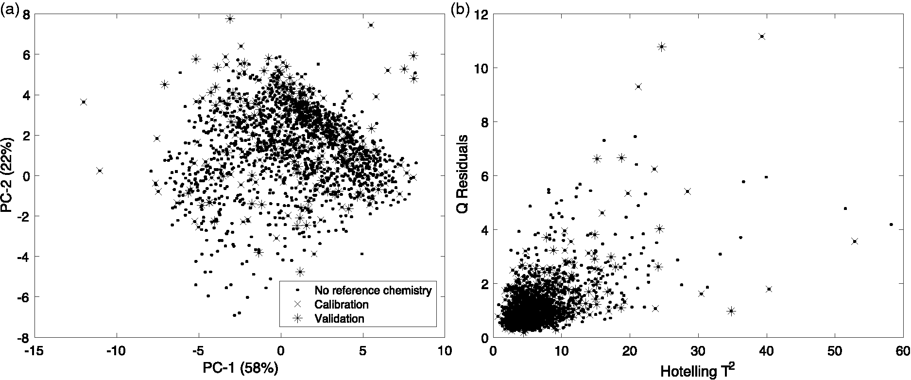
In a PCA of eucalypt dataset, the first two principal components explained 71% of the variation in NIR spectra (PC-1 = 54% and PC-2 = 16%). The SELECT function identified 987 samples for N_A analysis that distributed approximately uniformly across the spectral space of field season one (Figure 2). There were no gross outliers found in the plots of PC (Figure 2(a)) nor in the Q residuals vs. Hotelling T² statistic (Q vs. T², Figure 2(b)). For the Q vs. T² plot, seven PC factors that captured 90% of spectral variance were chosen. With so many samples it is to be expected that there will be a good deal of scatter in both the scores plot and the Q vs. T² plot. There were no points that separated from the rest of the data in either case, and so it was preferred to not exclude any data on the basis of these plots.

Figure 2.

(a) Distribution of scores of the available nitrogen spectral dataset along the first two principal components. (b) Q-residuals versus Hotelling T² within-model distances. Principal component analysis (PCA) was performed on the landscape eucalypt dataset (N = 2096, samples marked by “.”) and 987 samples were selected for calibration development (marked by “×”). Spectral data from three independent validation sets were projected onto the PCA space of the landscape eucalypt data (marked by “”, “” and “”). For the plot of Q vs. T², seven PC factors that captured 90% of spectral variance were chosen.

Samples from the states of Queensland (Qld), Victoria (Vic) and New South Wales (NSW) separated across PC-1 and PC-2 whereas samples from South Australia (SA) appeared to form compact clusters (Supplementary material 4a). While samples from the same local government area (e.g. Kangaroo Island) appeared to cluster (Supplementary material 4b), there were no other obvious clusters with subgenera (Supplementary material 4c), tree species (Supplementary material 4d), sample site (Supplementary material 4e), tree height (Supplementary material 4f) or DBH (Supplementary material 4g). Spectra acquired for samples in the three validation sets do not stand out as different from the training samples in either of the plots (Figure 2). Some samples from Validation1 separated along PC-2, and from the rest of reference value data (south east region of Figure 3(a)).

Figure 3.

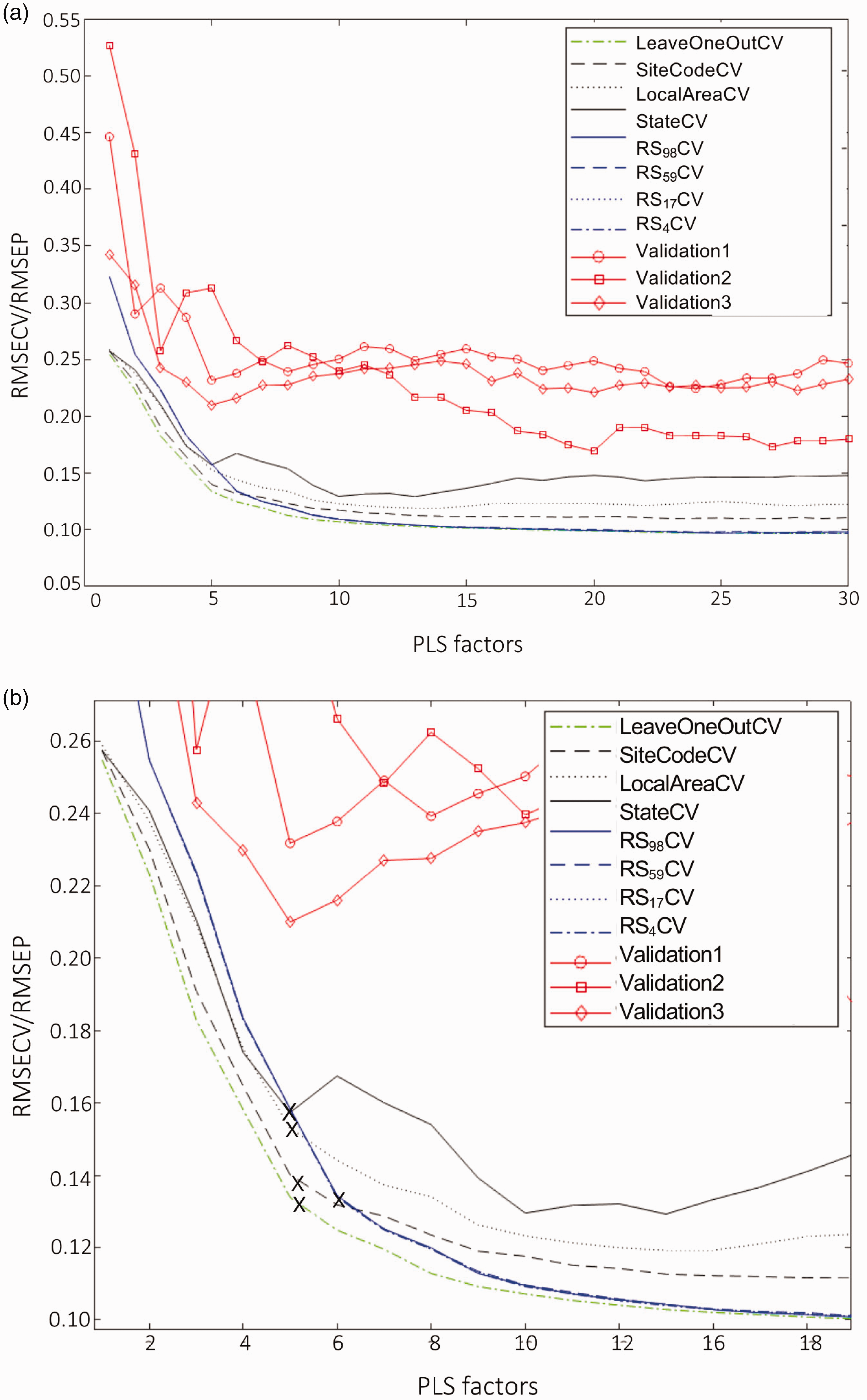
Comparing cross-validation techniques on the landscape eucalypt study and testing the calibration set against three independent validation sets. (a) Eight cross-validation techniques were tested for calibration model development and the key area is enlarged in (b). The techniques used were Leave-one-out (green line), Leave-group-out (black lines, splitting data by SiteCode, LocalArea and Australian State), Random subset division (blue lines, RS10 [98 groups], SiteCode [59 groups], LocalArea [17 groups], State [4 groups]. The predictive capability of the calibration set was tested against three validation sets using the RMSEP of the validation sets (red lines with markers). “×” indicates the selection of the number of PLS factors selected for the calibration models.

Calibration model development: Using the nested structure

Given that spectra clustered with local government area, the reference value data were split based on geographic nested structure and Table 2 summarises the calibration and validation results. The RMSECV of the calibration sets and the RMSEP of the split-off validation sets ranged from 0.12–0.18% N_A (Table 2). Predicting N_A in samples from a different Australian state provided the weakest predictions (highest error) during calibration development. This was demonstrated in both the State_CV (Table 2, RMSECV = 0.15–0.17% N_A) and when predicting N_A in an Australian state different to those in the calibration (Table 2, RMSEP = 0.15–0.18% N_A).

Table 2.

Performance of calibration models with different splits of the reference chemistry set.

		PLS factors	Calibration		Validation
Type of split	CV type	PLS factors	N	RMSECV	N	RMSEP
Random	Leave One Out	5	618	0.13	369	0.13
	SiteCode	5		0.14		0.13
	LocalArea	6		0.14		0.13
	State	5		0.15		0.13
	RS98	6		0.13		0.13
	RS59	6		0.13		0.13
	RS17	6		0.13		0.13
	RS4	6		0.13		0.13
Site code	Leave One Out	5	618	0.12	369	0.14
	SiteCode	5		0.14		0.14
	LocalArea	5		0.15		0.14
	State	5		0.16		0.14
	RS98	6		0.13		0.13
	RS59	6		0.13		0.13
	RS17	6		0.13		0.13
	RS4	6		0.13		0.13
Leave NSW out^a	Leave One Out	5	622	0.12	365	0.17
	SiteCode	5		0.13		0.17
	LocalArea	5		0.15		0.17
	State	5		0.16		0.17
	RS98	6		0.12		0.17
	RS59	6		0.12		0.17
	RS17	6		0.12		0.17
	RS4	6		0.12		0.17
Leave Qld out^b	Leave One Out	6	490	0.13	497	0.18
	SiteCode	5		0.15		0.15
	LocalArea	5		0.17		0.15
	State	5		0.15		0.15
	RS98	7		0.13		0.17
	RS59	7		0.13		0.17
	RS17	7		0.13		0.17
	RS4	7		0.13		0.17
All samples	Leave One Out	5	987	0.13	NA
	SiteCode	5		0.14
	LocalArea	5		0.15
	State	5		0.16
	RS98	6		0.13
	RS59	6		0.13
	RS17	6		0.13
	RS4	6		0.13

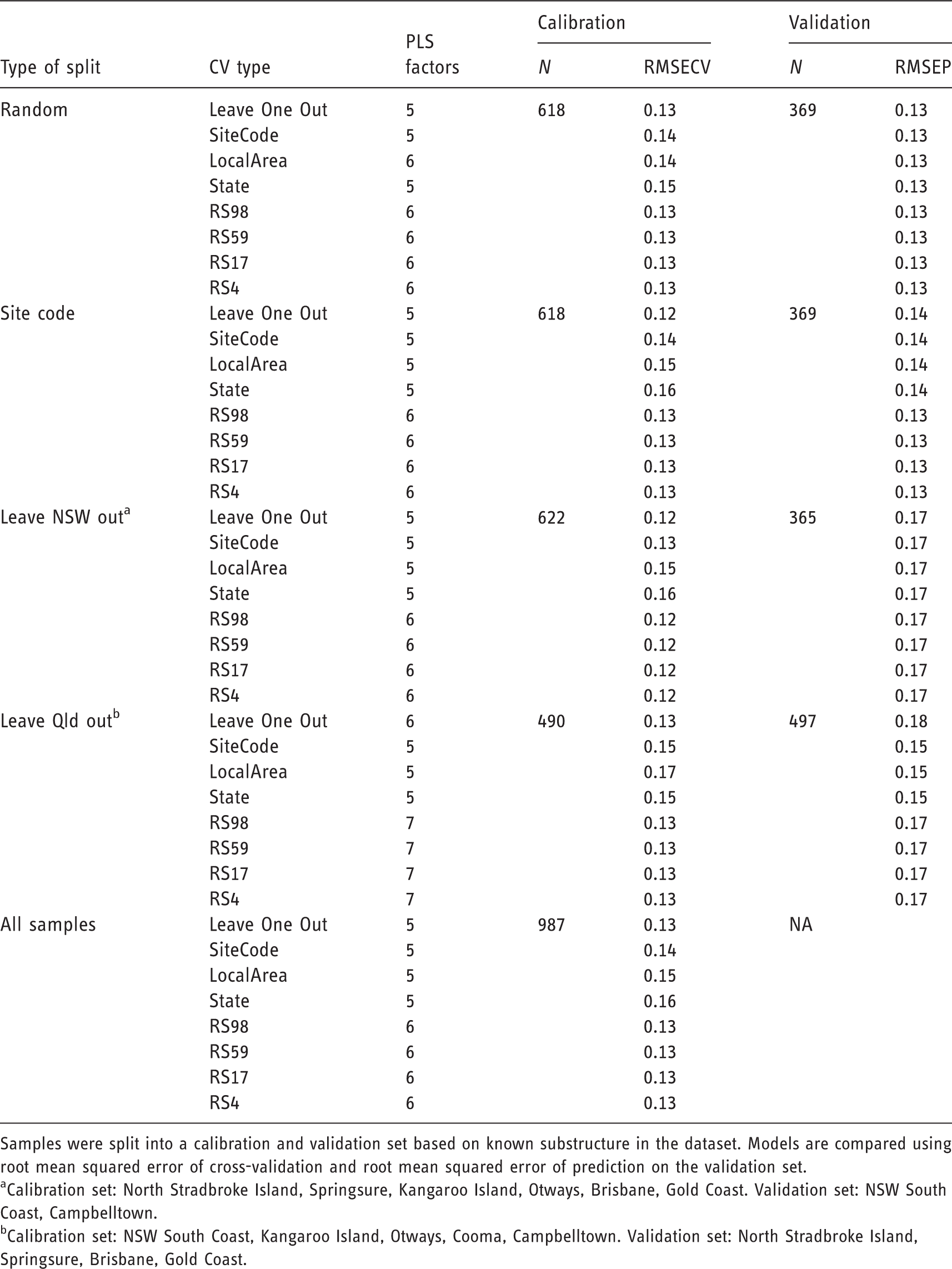
Samples were split into a calibration and validation set based on known substructure in the dataset. Models are compared using root mean squared error of cross-validation and root mean squared error of prediction on the validation set.

^aCalibration set: North Stradbroke Island, Springsure, Kangaroo Island, Otways, Brisbane, Gold Coast. Validation set: NSW South Coast, Campbelltown.

^bCalibration set: NSW South Coast, Kangaroo Island, Otways, Cooma, Campbelltown. Validation set: North Stradbroke Island, Springsure, Brisbane, Gold Coast.

All 987 reference value samples were then recombined to develop a global PLS model. The previously described eight cross-validation techniques were first tested on the large eucalypt dataset (Table 2). LOO_CV had the lowest RMSECV vs PLS factors curve, while State_CV had the highest curve, with a difference of about 0.03% N_A between curves (Figure 3(a) and (b)). RS_cv (Random Subset cross-validation) of the data, regardless of the size of the subsets, did not influence the cross-validation error of the model. The shape of the RMSECV curves differed between the cross-validation techniques. In the case of LOO_cv and LGO_cv, a “bend” in the curve indicated that five latent factors were suitable for building the model (Figure 3). However, in RS_cv six latent factors were chosen and it was found that the RMSECV curve of RS_cv continued to decrease until 22 latent factors. The RMSECV of all eight cross-validation techniques ranged from 0.12 to 0.17 (Figure 3).

The performance of two calibration models were compared, one with five and one with six PLS factors and the models were tested against the three independent validation sets (Figure 4). All independent validation samples were collected from sites in different local government areas to the calibration set. There was clear prediction bias for Validation1 (Figure 4(a) and (b)), while the model performed well for most samples in Validation2 (Figure 4(c) and (d)) and Validation3 (Figure 4(e) and (f)). The RMSEP across all three independent validation sets ranged from 0.21 to 0.31% N_A, approximately 50% greater error than the RMSECV curves (Figure 3(a)). No correlation was observed between the predictive error of the models and Mahalanobis distance from the mean spectra. A large Mahalanobis distance was not necessarily indicative of a large predictive error. No consistent relationship was also found between position in the Q vs T² plot and whether or not a sample predicted well (contribution to RMSEP). For example, outliers from Validation1 in the Q vs T² plot (Figure 2(b)) were predicted well with the calibration model (Figure 4(a) and (d)). Contrastingly, the model poorly predicted five samples (Figure 5(c) and (f)) and these samples were in fact inliers in Q vs T² plot (Figure 2(b)). These samples had relatively small Mahalanobis distances from the mean spectra and were located near many reference value samples. It is unknown why these samples were unique or different from the rest of the samples in this dataset. They were neither unique in collection site, tree species, Australian state nor chemistry.

Figure 4.

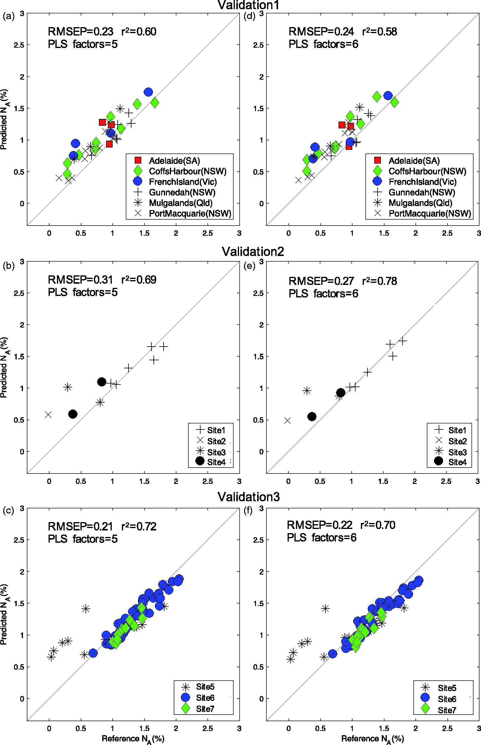
The relationship between reference and predicted available nitrogen (N_A) (%) across three independent validation sets. Samples were collected from New South Wales (NSW), Queensland (Qld), Victoria (Vic) and South Australia (SA). For each validation set, two separate calibration models were used, (a) to (c) models fitted with five PLS factors and (d) to (f) models fitted with six PLS factors. Data were fitted against a 45° line. Data points are marked by different sample sites within the validation set.

Figure 5.

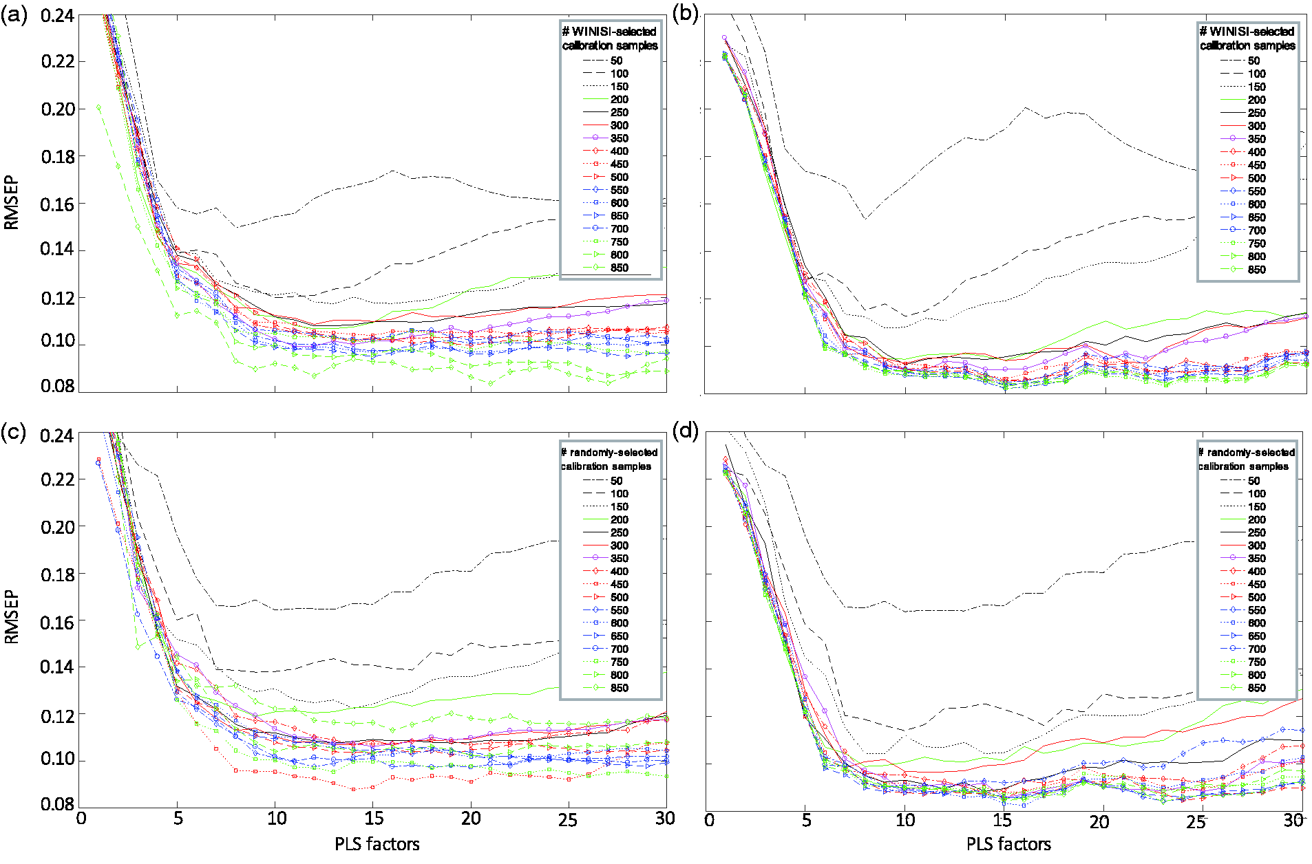
The change in the error prediction (RMSEP) of a model with an increasing number of calibration samples during model development. Using the reference chemistry samples from the landscape eucalypt study (N = 987), 886 samples with reference chemistry were allocated to a model development set (MDS) and 101 samples for a separate validation set. Calibration models were developed with an increasing number of samples (in increments of 50 samples) and increasing number of PLS factors. Models using the “SELECT” function in WINISI to select calibration samples from the MDS were (a) tested against the remaining samples in MDS and (b) against the set-aside validation set. Models which randomly selected calibration samples from the MDS were (c) tested against the remaining samples in the MDS and (d) against the set-aside validation set.

Given that different cross-validation techniques indicated different numbers of “optimal” PLS factors, the effect of the number of PLS factors on the prediction capability of the reference value data was investigated (Figure 3(a)). In all, 30 models were generated, with 1 to 30 PLS factors, and were tested against all three validation sets. For Validation1 and Validation3, the lowest predictive error was achieved using a model with five PLS factors. It was found that the RMSECV curve for State_CV was most useful as it best resembled the predictive error in these two RMSEP curves (Figure 3(a)). For Validation2, selecting an appropriate number of factors to build the model was difficult because the RMSEP curve continued to decrease until 20 factors were included. LOO_CV was found to be the least useful RMSECV curve as the RMSECV values were lower than any other RMSECV curve (Figure 3), and suggested cross-validation errors that were overly-optimistic when compared with the RMSEP of the three validation sets (Table 2, Figure 4).

Calibration model development: How many samples do we really need?

Throughout the study, a strong relationship was found between available nitrogen and NIR spectra when using a large number of reference value samples in the model (from 490 to 987 samples, Table 2). Similar results were found whether samples were selected randomly or based on Mahalanobis distance (Figure 5(a) to (d)). Changes to the number of calibration samples and PLS factors in the model influenced the prediction performance of the model (Figure 6(a) to (d)). From 200 samples on, the models appeared to become stable. Generally, including up to seven PLS factors showed smaller prediction errors on both the split-off validation set (the remaining samples in the model development set, Figure 5(a)) and the set aside validation set (Figure 5(b), N = 101 samples). The prediction error of the split-off validation set became smaller as the number of calibration samples increased and as the number of split-off validation samples decreased (Figure 5(a) and (c)). Contrastingly, including more samples during calibration did not necessarily improve the prediction performance of the model on the set-aside validation set. The prediction error on the set-aside validation set plateaued when including 300 or more calibration samples (Figure 5(b) and (d)).

Figure 6.

(a) Distribution of scores of the formylated phloroglucinol compounds (FPCs) spectral dataset along the first two principal components. (b) Q-residuals versus Hotelling T² within-model distances. Principal component analysis (PCA) was performed on the Symphyomyrtus dataset (N = 1605, samples marked by “.”) and 329 samples were selected for FPC analysis. Of these samples, 200 samples were randomly allocated for the calibration set (marked by “x”) and 129 samples for the validation set (marked by “*”. For the plot of Q vs. T², seven PC factors that captured 93% of spectral variance were chosen.

Formylated phloroglucinol compounds

Diversity of FPC chemical profiles

The eucalypt dataset included 38 species, never before analysed for FPCs. These samples were collected across four different Australian states, Qld, NSW, Vic and SA. The reference library included a diverse range of FPC chemical profiles. Evidence of three common chemical profiles²⁶ were found, as well as unique chemical profiles whose eluting peaks remain unidentified.

Spectra

In a PCA of Symphyomyrtus samples from the FPC Dataset, 80% of the spectral variation in NIR spectra was explained by the first two principal components (Figure 6(a)). The reference value samples separated across PC-1 and PC-2 and there were no stand-out differences between the calibration and validation sets (Figure 6). There were no gross outliers found in the plots of PC (Figure 6(a)) nor in the Q vs. T² (Figure 6(b)) and so no data were excluded. For the Q vs. T² plot, seven PC factors that captured 93% of spectral variance were chosen.

Calibration model development: Do you need every compound?

A calibration was developed with the sum of the 17 FPCs, TotalFPCs₁₇. The LOO_CV cross-validation results indicated a PLS model with 14 factors was adequate to explain the variance between TotalFPCs₁₇ and NIR spectra. The RMSECV on the calibration set was 4.4 mg.kg⁻¹ and RMSEP on the independent validation set was 4.7 mg.kg⁻¹ (Figure 7(a)).

Figure 7.

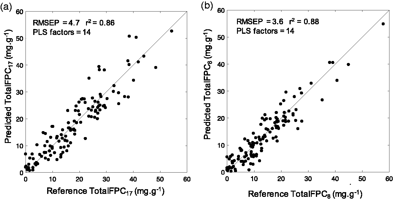
The relationship between reference and predicted formylated phloroglucinol compounds (FPCs, mg.g⁻¹). Separate calibration models were developed to predict two indexes of FPCs, (a) TotalFPCs₁₇ which includes 17 FPC compounds and (b) TotalFPCs₈ which includes eight FPC compounds identified to have a high covariance with near infrared spectra. Data were fitted against a 45° line.

PLS2 with 17 known FPCs was carried out to investigate which FPCs co-varied with the NIR spectra. For the first four PLS factors, eight compounds had a high covariance (Y loadings) with the NIR spectra (Figure 8): eucalyptone, macrocarpal 34, grandinal 44, sideroxylonal A, sideroxylonal C, grandinal 54, macrocarpal A and macrocarpal G. These eight compounds were summed for a new index of FPCs, TotalFPCs₈. There was an improvement on the predictive power of the calibration model with 14 PLS factors. The RMSECV on the calibration set was reduced to 3.7 mg.kg⁻¹ and RMSEP on the independent validation set was reduced to 3.6 mg.kg⁻¹ (Figure 7(b)). The coefficient of variation of the RMSEP between the two FPC indexes was around 30%, indicating that the prediction error across both indexes of FPCs were similar.

Figure 8.

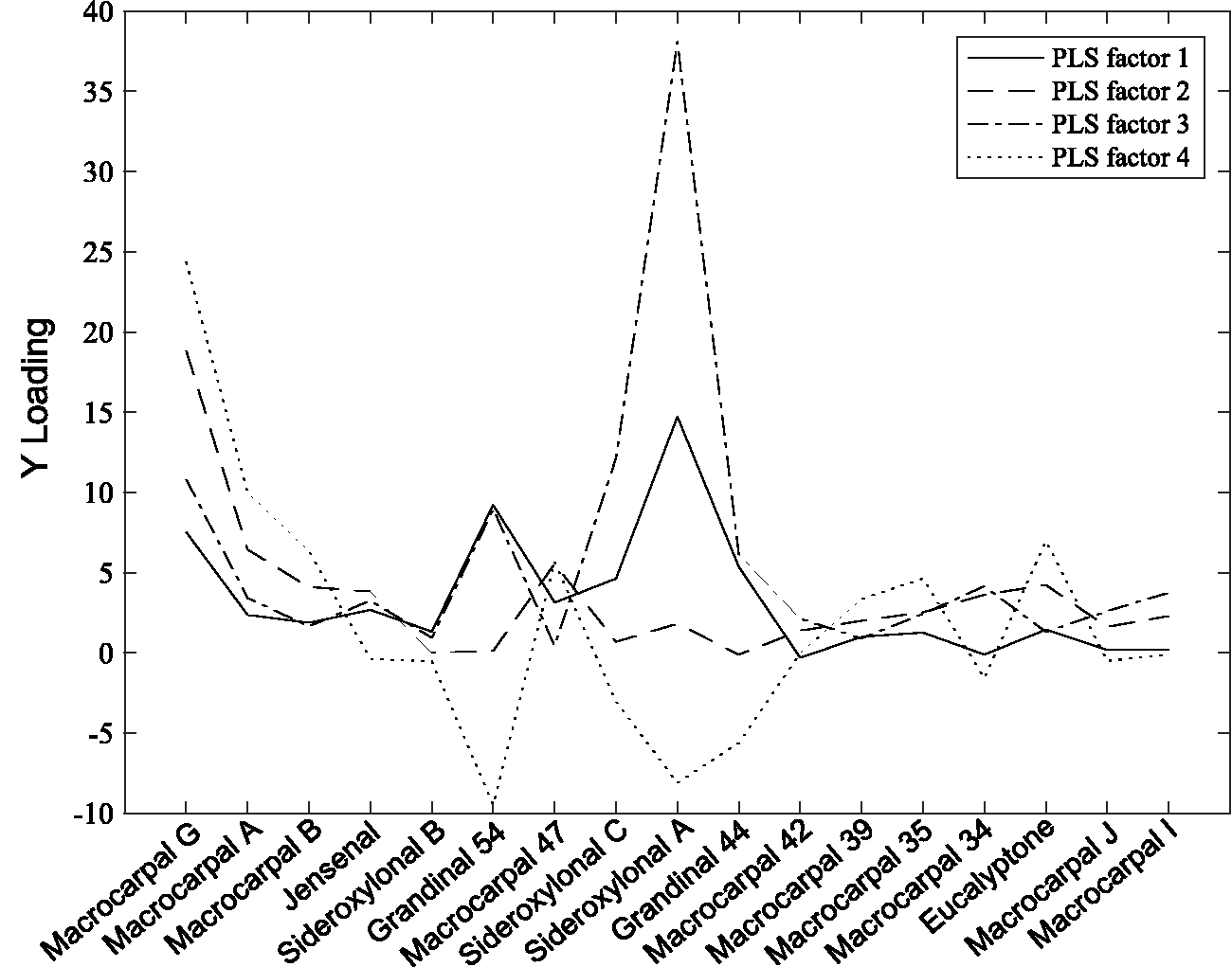
PLS2 on TotalFPCs₁₇ with near infrared spectra. The covariance (Y loadings) of each formylated phloroglucinol compound (FPC) with spectral data across the first four partial least square (PLS) factors.

Discussion

This study examined a variety of model development and validation techniques, illustrating different approaches one can use when building broad-based calibrations with large datasets. Furthermore, the work highlights the power of NIR spectroscopy and multivariate analysis to guide analytical work for complex ecologically-relevant traits.

Available nitrogen: Using the nested structure

The collection sites spanned thousands of kilometres, across eastern and southern Australia (Figure 1), and contained leaf samples from areas and eucalypt species that have never been assessed for nutritional quality. This study explored what types of nested structure could exist in large datasets. The large N_A dataset included 80 eucalypt species from eastern and southern Australia and was highly valuable for building a broad-based N_A calibration. The PCA analysis of the N_A dataset revealed that samples from the same local government area and Australian state clustered to varying degrees in spectral space (Supplementary material 4a, b) and suggested that samples from similar geographic areas may share similar spectral properties. This spatial structure was used during cross-validation and validation. Within the study, the typical pattern found was that regardless of how the eucalypt reference value data was split, the RMSECV and RMSEP values matched well across each test (Table 2). When local government area or Australian state was taken into account, the largest differences between RMSECV and RMSEP were found, with the predictive errors being about 0.02–0.03% N_A (about 20%) greater. It is not unusual to find geographically-similar spectra clumping together during PCA.¹⁴ Thus, there are probably spectral properties within different geographic areas that make samples unique and this could be very useful during model development.

Geographic location is an easy marker that can act as a surrogate for more fundamental, and typically confounding, variables such as plant species, climate zone and soil. Thus, a simple classification of geography will allow researchers to account for different types of variability that are typically difficult to separate. Secondly, access to soil, plant species or climate data is not always possible to collect. However, researchers will know the sample collection location and can use this structure during calibration development. Finally, cross-validating a model based on geographic variation is more in line with the future aims of the calibration. The aim of this study is to predict samples in a new project, and this is typically associated with geographic location.

A broad-based calibration model is more robust if it includes samples from a variety of locations and plant species to capture as much spectral variation as possible. To develop a robust N_A calibration model that covered the range of the large Eucalypt Database, all reference value data (N = 987, Table 2) were combined. During the exploratory process, most validation samples overlapped with the reference value data and a few samples from Validation1 separated out in the south-east region (Figure 2(a)). Given that most independent validation samples were within the spectral space of the reference value data, it was expected that the calibration model would perform well for these samples.²⁷ Despite finding strong relationships with N_A and NIR spectra within the reference value dataset and knowing that this relationship exists in many other previous studies, a reduction in prediction accuracy against independent samples was still experienced. The prediction errors of independent samples were up to 50% greater than that found during calibration development, indicating that the model was somewhat limited when predicting these samples (Figure 4). It is also useful to highlight that the RMSECV results from LOO_CV were the least useful for assessing the model’s ability to predict the validation samples, and this is likely due to pseudo-replicates within geographic location. Thus, the use of LOO_CV is discouraged in large datasets as it is likely to lead to low RMSECV values that do not reflect the predictive error of the model.

Large datasets are invaluable as the heterogeneity of the samples can represent the large natural variability of the study system. However, as new geographic variables or species are introduced to a calibration model, it is likely that unique spectral properties will be encountered which could affect the modelled relationship found between spectra and the chemical trait (non-linear effects). Moreover, it may not be clear which samples are needed to broaden the model. For example, the calibration models in this study performed well for most samples, but it is unknown why the models performed poorly for five independent samples in Validation3 (Figure 4(e) and (f)). These poorly-predicted samples were largely within the spectral space of the large eucalypt database and were not unique in terms of chemistry, tree species or broad geographic location. Whether exploratory plots (Figure 2) could help us identify areas where the model performed poorly was investigated. However, an inconsistent relationship was found between a sample’s position on a Q vs. T² plot and how well a sample could be predicted. This suggests that a spectral outlier does not necessarily indicate that it will be predicted poorly. Thus, it is difficult to assess how well a model has captured the variability of the study system and how it can perform for new samples.

Typically, a drop in prediction accuracy is seen when the model is applied to independent samples, indicating that not all the natural variability in the study system is accounted for in the model. This has been found when building global calibration models for the freshness of albumen,⁵ the cellulose content of eucalypts,³ and properties of pine wood² and forage quality¹ and digestibility.³⁵ A general approach is to include some of the independent validation samples to extend the scope of the model, and this study cautions the use of this method. While this approach (known as a model extension or augmentation) makes the current prediction statistics better, this would require a new independent validation set to test if the predictive performance of the model is indeed better. A drop in prediction accuracy could also reflect variation in data collection. There can be considerable differences between laboratory instruments and users which could lead to prediction bias in new samples.^1–3 It is possible that the prediction bias found in Validation1 could be related to differences between technicians when performing the N_A assay. In this study, the same technician performed N_A analysis on the calibration set, Validation2 and Validation3, while a different technician collected the N_A data for Validation1.

Robust or accurate?

Accurate NIR models that predict complex traits are essential for ecological, silviculture agricultural and botanical studies, yet deciding if and when a model is accurate enough is difficult without knowing exactly what purpose the data will serve. There is limited information on the predictive error of calibration models in ecological studies. Models are typically described by their cross-validation error which is then extrapolated to predictive error for the remaining samples.^9,11,12,15 From RMSECV results only, an error between 0.12 and 0.17% N_A can be expected from this study. The upper range of the RMSECV (0.12–0.17% N_A) is considerably higher than the RMSECV previously reported in other NIR calibration statistics for these chemical constituents (ranging from 0.07 to 0.13% N_A).^{9,10,12,14,15} When testing the models on three independent validation sets, the RMSEP ranged from 0.21 to 0.31% N_A, considerably higher than the RMSECV values. Thus, these results suggest that the current N_A models can predict eucalypt samples from independent datasets with a prediction error range of 0.12–0.31% N_A. These predictive errors are considered acceptable as the eucalypt dataset had a mean of 1% N_A with a range of 0.2–2.7% – considerably wider than that of previous studies (the average N_A in other ecological studies ranges from 0.2 to 0.72%).

The accuracy tolerance of the calibration model is application dependent. Many important ecological effects depend on relatively small differences between samples, sites or seasons. For example, subtle differences of 0.1–0.2% N_A in the average concentration of N_A across the home ranges of female brushtail possums have a substantial impact on their reproductive success.¹² The prediction error of the eucalypt model was 0.13–0.31% N_A, and it is possible that it may not be accurate enough to detect small mean differences of the home ranges of animals in DeGabriel’s study.¹² In the case of a landscape scale project where the comparisons are between sites that vary over a much larger scale, the accuracy tolerance of an NIR calibration model might not be as strict. To the authors’ knowledge, this is yet to be investigated in ecology due to the difficulties associated with collecting chemical data across landscapes. The large Eucalypt Dataset will provide an opportunity to explore the accuracy thresholds required to explain differences in animal abundance and distribution. It is recognised that the most valid calibration method is dependent on what the user intends to achieve with the calibration model; predicting a single dataset accurately or predicting a broad range of datasets adequately.

Available nitrogen: How many samples do you really need?

Accounting for spectral variation is essential for a robust model. However, constructing the initial calibration set for this study based on spectral variation (using the SELECT algorithm) as the major criterion resulted in an excessive number of calibration samples for N_A. This is a common technique for selecting samples and this study suggested that it may not be very efficient. The results that compared split-off and set-aside validation sets suggested that a set-aside validation set is important for determining how many samples are required to efficiently build a calibration model (Figure 5). When testing the split-off validation set, the prediction error continued to decrease as more samples were included in the calibration. During the split-off validation test, more and more spectrally variable samples were selected for the calibration set. Consequently, those samples left-behind to validate the model were less variable, hence, the decrease in prediction error. While predicting these “left-behind” samples is likely to leave users with great calibration statistics, it is also likely to tempt users to chase a prediction accuracy that may be overly optimistic. With the set-aside validation set, however, prediction error dropped off around 0.1% N_A and little improvement in prediction accuracy was found from including 300 to 850 calibration samples. This indicated that equivalent calibrations could be achieved with only 30% of the reference value data. This is a concern as the general aim was to use NIR spectroscopy to efficiently get N_A values for the dataset and analysing hundreds more samples than required contrasts with that aim.

Simply relying on Mahalanobis distance to select samples may lead to an excess of reference value samples as the variation in N_A may not necessarily equal the variation in the spectral space of the dataset.³⁶ To the authors’ knowledge, this test has been rarely investigated in this field and so it is unknown how frequently this may happen in other studies. For future calibrations with chemical traits known to predict well with NIR spectra (such as N_A), this study suggests that users should start conservatively. Select a small number of samples for calibration development and then test the cross-validation performance of the model. If required, add additional reference value samples unique spectral and/or geographic properties to reduce the cross-validation error of the model.

Towards a global calibration

The complexity of a nutritional trait is likely to influence the feasibility of developing a broad-based calibration model for the trait. N_A is relatively simple to measure and can be compared across all eucalypt samples. In fact, N_A has distinguished some subgenera of Eucalyptus and has highlighted the range of inter- and intraspecific variation amongst eucalypt species.³⁷ Given that N_A is a common currency that can be used to compare across studies and sites, it is appropriate to use this dataset to investigate the potential challenges of a broad-based calibration model. However, there are many complex nutritional traits that are equally important for ecological studies and have their own NIR challenges. Here, some guidance is also provided on how to work with more complex traits using the FPC dataset.

Formylated phloroglucinol compounds: Do you need every compound?

FPCs are a highly diverse group of compounds that include different chemical classes and significant structural diversity both within and across species.^26,38 The variability of FPC profiles makes it an intrinsically more complex measurement. Due to this variability, researchers have focussed on developing separate FPC calibration models per eucalypt species. Using these single-species FPC models, researchers have detected many ecologically relevant patterns^30,38,39 and some studies have been validated with concurrent studies using isolated FPC compounds.⁴⁰ This study suggests that an FPC reference library that includes many different eucalypt species may enable the development of a broad-based FPC calibration model.

Using the reference method from Moore et al.²⁶ to quantify 17 FPC compounds, many studies have described how FPCs influence feeding behaviour and tree use in marsupial folivores.^9–11 A comprehensive calibration model was developed to predict TotalFPC₁₇ in 38 different Symphyomyrtus species collected over a wide geographic range. The predictive error of this TotalFPC₁₇ model (RMSECV = 4.4–4.7 mg.g⁻¹) resembled those found in site-specific ecological studies with only one to three eucalypt species (with SECV ranging from 2.4 to 5.8 mg.g⁻¹).^9,11 Thus, this TotalFPC₁₇ model is likely to be valuable for future ecological studies and this study demonstrates that it is possible to build a robust and reliable multi-species and multi-site FPC calibration.

Although the Total FPC₁₇ calibration model is suitable for a broad landscape study, it will most likely require ongoing expansion and maintenance. Some eucalypt species were investigated here for the first time and unique chemical profiles that are yet to be recorded in the literature were found. This suggests that the current reference method may be limited and that there may be a need to invest significant resources in isolating and purifying additional standards. In particular, the widely-distributed E tereticornis showed several late eluting peaks that may be unknown FPCs and these prominent unknown peaks appeared to be characteristic of this species. Indeed, recent research has reported several new FPCs from this species.⁴¹ Given that it is likely that researchers will need to include additional individual compounds to the FPC index, it would be valuable to identify potential sources of error during FPC calibration development.

Complex chemical traits, such as FPCs, are difficult to measure because obtaining standards for individual compounds for HPLC analysis can be a time-consuming and expensive process. The use of PLS2 highlighted potential sources of error associated with the 17 individual FPC compounds during calibration development. The covariance between FPC compounds and NIR spectra differed between compounds. Eight compounds had a high covariance with NIR spectra, whereas nine other compounds showed little covariance (Figure 8). The eight compounds with high covariance tended to occur in larger concentrations and most (but not all) have suitable standards for HPLC analysis.²⁶ Contrastingly, the remaining nine compounds occurred at lower concentrations or were sparsely distributed and so have proven difficult to isolate for use as standards.²⁶ While it is clear that the ability to predict chemical traits relies on accurate reference samples to train the model, this study suggests the use of PLS2 to help identify potential sources of error within complex traits.

This study describes methods that would allow researchers to focus on a select number of FPC compounds and consequently reduce the costs associated with complex chemical trait analysis. It is likely that the reduced index of prominent FPCs, TotalFPCs₈ is valuable, however future studies are required to investigate if TotalFPCs₈ is as ecologically-important as TotalFPCs₁₇. Nonetheless, this study provides the first stepping stone towards a broad-based FPC calibration. Given that the concentration of FPCs and other defensive compounds can restrict how much an herbivore can eat^22,25 and explain animal distribution patterns,⁴² discovering strategies to better and more efficiently assess these compounds is likely to help support the management and conservation of animals.

Conclusions

Identifying the underlying causes of variation in large datasets can help build broad-based calibration models, facilitating the integration of NIR spectroscopy into many fields. This study proposes the use of different cross-validation techniques for model fitting and selection. Knowing how to better split reference value data and testing calibration models against different independent validation sets can lead to more realistic estimates of model predictive performance. Furthermore, this study suggests that assessing model performance while collecting reference value data may help researchers avoid analysing an excessive number of reference value samples for calibration development. Lastly, the study shows that it is possible to use PLS to highlight potential sources of error when building calibration models for complex chemical traits such as FPCs.

The application of the model is important when deciding how best to develop calibration models and assess model predictive performance. Those who wish to build a global model that covers large geographic variation and plant diversity are likely to make compromises on the predictive ability of their model. Nonetheless, the Eucalyptus database could provide a base for a global N_A calibration model. Given the importance of digestible protein in non-Australian study systems,^23,24 the N_A calibration model could be extended to nutritional ecology studies worldwide. Combining leaf samples from multiple projects in a single database would lead to an NIR library that encapsulates the variation of leaf samples for folivores across different countries. The authors’ acknowledge that this is an ambitious goal and challenges ahead would include standardization of reference methods and spectra collection across users and instruments. If this variation can be captured in a single, global calibration model, the number of samples required for chemical analyses in new projects could be significantly reduced and, thus, facilitate the integration of forage quality into ecological studies. To do this, future studies will need to investigate how this complexity may affect the development and accuracy of calibration models. This study has highlighted some potential cross-validation and validation techniques to tackle this.

Supplemental Material

JNS902536 Supplemental Material - Supplemental material for Sample selection, calibration and validation of models developed from a large dataset of near infrared spectra of tree leaves

Supplemental material, JNS902536 Supplemental Material for Sample selection, calibration and validation of models developed from a large dataset of near infrared spectra of tree leaves by Jessie Au, Kara N Youngentob, William J Foley, Ben D Moore and Tom Fearn in Journal of Near Infrared Spectroscopy

Footnotes

Acknowledgements

G. Batten, P. Kenny, R. Deans and C. McDonald-Spicer provided helpful comments on the manuscript.

Declaration of conflicting interests

The author(s) declared no potential conflicts of interest with respect to the research, authorship, and/or publication of this article.

Funding

The author(s) disclosed receipt of the following financial support for the research, authorship, and/or publication of this article: A National Environmental Research Program grant to KNY and a grant from NSW Department of Environment and Heritage to WJF funded this research. Travel grants from ANU Vice Chancellor and International Council of Near Infrared Spectroscopy funded JA.

ORCID iDs

Jessie Au

Tom Fearn

Supplemental material

Supplemental material for this article is available online.

References

1.
Berzaghi P Flinn PC Dardenne P , et al. Comparison of linear and non-linear near infrared calibration methods using large forage databases. In: Davies RK Cho (eds) Near infrared spectroscopy: proceedings of the 10th international conference. Chicester: NIR Publications, 2002, pp. 107–111.

2.
Schimleck LR Hodge GR Woodbridge W. Toward global calibrations for estimating the wood properties of tropical, sub-tropical and temperate pine species. J Near Infrared Spectrosc 2010; 18: 355–365.

3.
Downes G Meder R Harwood C. A multi-site, multi-species near infrared calibration for the prediction of cellulose content in eucalypt woodmeal. J Near Infrared Spectrosc 2010; 18: 381–387.

4.
Smith KF Flinn PC. Monitoring the performance of a broad-based calibration for measuring the nutritive value of two independent populations of pasture using near infrared reflectance (NIR) spectroscopy. Aust J Exp Agric 1991; 31: 205–210.

5.
Kemps BJ Saeys W Mertens K , et al. The importance of choosing the right validation strategy in inverse modelling. J Near Infrared Spectrosc 2010; 18: 231–237.

6.
Gillon D Houssard C , and Joffre R. Using near-infrared reflectance spectroscopy to predict carbon, nitrogen and phosphorus content in heterogeneous plant material. Oecologia 1999; 118, 173–182.

7.
Lawler IR Aragones L Berding N , et al. Near-infrared reflectance spectroscopy is a rapid, cost-effective predictor of seagrass nutrients. J Chem Ecol 2006; 32: 1353–1365.

8.
Vance CK Tolleson DR Kinoshita K , et al. Near infrared spectroscopy in wildlife and biodiversity. J Near Infrared Spectrosc 2016; 24: 1–25.

9.
Moore BD Foley WJ. Tree use by koalas in a chemically complex landscape. Nature 2005; 435: 488–490.

10.
Youngentob KN. Wallis IR Lindenmayer DB , et al. Foliage chemistry influences tree choice and landscape use of a gliding marsupial folivore. J Chem Ecol 2011; 37: 71–84.

11.
Marsh KJ Moore BD Wallis IR , et al. Feeding rates of a mammalian browser confirm the predictions of a ‘foodscape’ model of its habitat. Oecologia 2014; 174: 873–882.

12.
Degabriel JL Moore BD Foley WJ , et al. The effects of plant defensive chemistry on nutrient availability predict reproductive success in a mammal. Ecology 2009; 90: 711–719.

13.
Ebbers MJH Wallis IR Dury S , et al. Spectrometric prediction of secondary metabolites and nitrogen in fresh Eucalyptus foliage: towards remote sensing of the nutritional quality of foliage for leaf-eating marsupials. Aust J Bot 2002; 50: 761–768.

14.
Windley HR Foley WJ. Landscape-scale analysis of nutritional traits of New Zealand tree foliage using near-infrared spectroscopy. For Ecol Manage 2015; 357: 161–170.

15.
Stalenberg E Wallis IR Cunningham RB , et al. Nutritional correlates of koala persistence in a low-density population. PLoS One 2014; 9: e113930.

16.
Asner GP Martin RE Knapp DE , et al. Spectroscopy of canopy chemicals in humid tropical forests. Remote Sens Environ 2011; 115: 3587–3598.

17.
Dardenne P. Calibration transfer in near infrared spectroscopy. NIR News 2002; 13: 3–7.

18.
Stolter C Julkunen-Tiitto R Ganzhorn JU. Application of near infrared reflectance spectroscopy (NIRS) to assess some properties of a sub-arctic ecosystem. Basic Appl Ecol 2006; 7: 167–187.

19.
Rothman JM Chapman CA Hansen JL , et al. Rapid assessment of the nutritional value of foods eaten by mountain gorillas: applying near-infrared reflectance spectroscopy to primatology. Int J Primatol 2009; 30: 729–742.

20.
Wallis IR Edwards MJ Windley H , et al. Food for folivores: nutritional explanations linking diets to population density. Oecologia 2012; 169: 281–291.

21.
DeGabriel JL Moore BD Felton AM , et al. Translating nutritional ecology from the laboratory to the field: milestones in linking plant chemistry to population regulation in mammalian browsers. Oikos 2014; 123: 298–308.

22.
Marsh KJ Wallis IR Andrew RL , et al. The detoxification limitation hypothesis: where did it come from and where is it going? J Chem Ecol 2006; 32: 1247–1266.

23.
Spalinger DE Collins WB Hanley TA , et al. The impact of tannins on protein, dry matter, and energy digestion in moose (Alces alces). Can J Zool 2010; 88: 977–987.

24.
Felton AM Felton A Raubenheimer D , et al. Protein content of diets dictates the daily energy intake of a free-ranging primate. Behav Ecol 2009; 20: 685–690.

25.
Lawler IR Foley WJ Pass GJ , et al. Administration of a 5HT₃ receptor antagonist increases the intake of diets containing Eucalyptus secondary metabolites by marsupials. J Comp Physiol B 1998; 168: 611–618.

26.
Moore BD Wallis IR Palá-Paul J , et al. Antiherbivore chemistry of Eucalyptus – cues and deterrents for marsupial folivores. J Chem Ecol 2004; 30: 1743–1769.

27.
Naes T Isakson T Fearn T , et al. A user-friendly guide to multivariate calibration and classification. Chichester: NIR Publications, 2002.

28.
Martens H Naes T. Multivariate calibration. New York: Wiley, 1989.

29.
Fearn T. Independent validation sets. NIR News 2013; 24: 19–20.

30.
Moore BD Foley WJ Wallis IR , et al. Eucalyptus foliar chemistry explains selective feeding by koalas. Biol Lett 2005; 1: 64–67.

31.
Youngentob KN Zdenek C van Gorsel E. A simple and effective method to collect leaves and seeds from tall trees. Methods Ecol Evol 2016; 7: 1119–1123.

32.
DeGabriel JL Wallis IR Moore BD , et al. A simple, integrative assay to quantify nutritional quality of browses for herbivores. Oecologia 2008; 15: 107–116.

33.
Savitzky A Golay MJE. Smoothing and differentiation of data by simplified least squares procedures. Anal Chem 1964; 36: 1627–1639.

34.
Fearn T Perez-Marin DC Garrido-Varo A , et al. Inverse, classical, empirical and non-parametric calibrations in a Bayesian framework. J Near Infrared Spectrosc 2010; 18: 27–38.

35.
Coates DB Dixon RM. Developing robust faecal near infrared spectroscopy calibrations to predict diet dry matter digestibility in cattle consuming tropical forages. J Near Infrared Spectrosc. 2011; 19: 507–519.

36.
Fearn T. Limitations of Mahalanobis and H distances. NIR News 2011; 22: 16.

37.
Wallis IR Nicolle Foley WJ. Available and not total nitrogen in leaves explains key chemical differences between the eucalypt subgenera. For Ecol Manage 2010; 260: 814–821.

38.
Wallis IR Keszei A Henery ML , et al. A chemical perspective on the evolution of variation in Eucalyptus globulus. Perspect Plant Ecol Evol Syst 2011; 13: 305–318.

39.
Marsh KJ Wallis I Foley WJ. Behavioural contributions to the regulated intake of plant secondary metabolites in koalas. Oecologia 2007; 154: 283–290.

40.
Lawler IR Foley WJ Eschler BM , et al. Foliar concentration of a single toxin creates habitat patchiness for a marsupial folivore. Ecology 2000; 81: 1327–1338.

41.
Liu H Feng MY Yu Q , et al. Formyl phloroglucinol meroterpenoids from Eucalyptus tereticornis and their bioactivities. Tetrahedron 2018; 74: 1540–1545.

42.
Bryant JP Clausen TP Swihart RL , et al. Fire drives transcontinental variation in tree birch defense against browsing by snowshoe hares. Am Nat 2009; 174: 13–23.

Supplementary Material

Please find the following supplemental material available below.

For Open Access articles published under a Creative Commons License, all supplemental material carries the same license as the article it is associated with.

For non-Open Access articles published, all supplemental material carries a non-exclusive license, and permission requests for re-use of supplemental material or any part of supplemental material shall be sent directly to the copyright owner as specified in the copyright notice associated with the article.

0.00 MB

1.10 MB

Sample selection,calibration and validation of models developed from a large dataset of near infrared spectra of tree leaves

Abstract

Keywords

Introduction

An ecological study – Eucalypt forage quality

Calibration development and model validation

Aims

Available nitrogen: Using the nested structure

Available nitrogen: How many calibration samples do you really need?

FPC calibration: Do you need every compound?

Methods and materials

Sample collection

Sample preparation and spectral collection

Available nitrogen

Calibration data description and selection

Spectral pretreatments

Calibration development and internal validation: Using the nested structure

External validation

Calibration development and validation: How many samples do you really need?

Formylated phloroglucinol compounds

Calibration data description and selection

Calibration development and validation: Do you need every FPC compound?

Results

Available nitrogen

Spectra

Calibration model development: Using the nested structure

Calibration model development: How many samples do we really need?

Formylated phloroglucinol compounds

Diversity of FPC chemical profiles

Spectra

Calibration model development: Do you need every compound?

Discussion

Available nitrogen: Using the nested structure

Robust or accurate?

Available nitrogen: How many samples do you really need?

Towards a global calibration

Formylated phloroglucinol compounds: Do you need every compound?

Conclusions

Supplemental Material

JNS902536 Supplemental Material - Supplemental material for Sample selection, calibration and validation of models developed from a large dataset of near infrared spectra of tree leaves

Footnotes

Acknowledgements

Declaration of conflicting interests

Funding

ORCID iDs

Supplemental material

References

Supplementary Material