
Abstract
Interest in the processes that mediate between stimuli and responses is at the heart of most modern psychology and neuroscience. These processes cannot be directly measured but instead must be inferred from observed responses. Race models, through their ability to account for both response choices and response times, have been a key enabler of such inferences. Examples of such models appeared contemporaneously with the cognitive revolution, and since then have become increasingly prominent and elaborated, so that psychologists now have a powerful array of race models at their disposal. We showcase the state of the art for race models and describe why and how they are used.
Keywords
Quantitative models express psychological theories in a way that facilitates rigorously testing them against data. This article reviews an influential and widely used type of quantitative psychological model, the race model. Figure 1 illustrates one of the most well-known examples, Logan and Cowan’s (1984) horse-race model of the stop-signal task, used to measure the ability to inhibit a response. The “horses” represent cognitive processes racing against each other; if the “go” runner wins, a response is made, and if the “stop” runner wins, it is withheld. The speed of the stop runner is the key measure of inhibitory ability, but by definition, that runner’s finishing time is not observable. However, combining what can be observed with assumptions based on the horse-race model enables estimation of the stop runner’s speed. Measuring the unobservable in this way exemplifies the role of race models in inferring psychological quantities that cannot be directly observed.
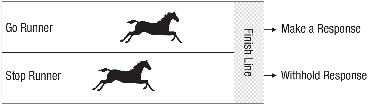
Logan and Cowan’s (1984) horse-race model of response inhibition in the stop-signal task. On most trials (go trials), participants perform a choice task, making a response (typically a binary choice) to a go stimulus, but on some trials, a stop signal (e.g., a tone) also occurs some time after the go stimulus, indicating that they should withhold their response. Typically, the delay between the go and stop signals is varied, and its effects on the probability of stopping and response times (RTs) when stopping fails, along with RTs when there is no stop signal, are observed. The “horses” represent cognitive processes racing toward the finish line; if the go runner wins, a response is made, and if the stop runner wins, it is withheld. Combining the race model with these observables, along with some assumptions about the distribution of finishing times, provides an estimate of stop-signal RT, the time it takes the stop horse to run the race.
What Are Race Models?
The defining characteristics of a race model are that (a) it contains one or more “runners” that take time to complete the race; (b) if there are two or more runners, they may or may not interact in a way that affects their timing; and (c) it acts according to a winner-takes-all rule that controls subsequent processing on the basis of the runner, or set of runners, that finishes first. Evidence-accumulation models (EAMs) are the most widely adopted special case of a race model. In EAMs, the runners have a specific interpretation as processes that are completed when they have accrued a threshold amount of evidence. We first examine several basic EAMs used to model simple decision tasks. We then describe how these basic EAMs can be used as building blocks to study a broader range of tasks and psychological processes.
Figure 2 illustrates three race models, two in which the runners are independent, the linear ballistic accumulator (LBA) and the racing diffusion model (RDM), and one that is a special case of the latter, the Wiener diffusion model (WDM), in which the runners interact. In the LBA and RDM, the horses are evidence accumulators, and each accumulator’s position is the current value of the sum of the evidence for the response that accumulator represents. For example, if the task involves a choice about whether a stimulus is moving to the left or right, the model could have accumulators corresponding to the two response options, as shown in Figure 2. Accumulation rates vary from trial to trial but are on average higher for the accumulator that matches the stimulus than for the accumulator that mismatches the stimulus.
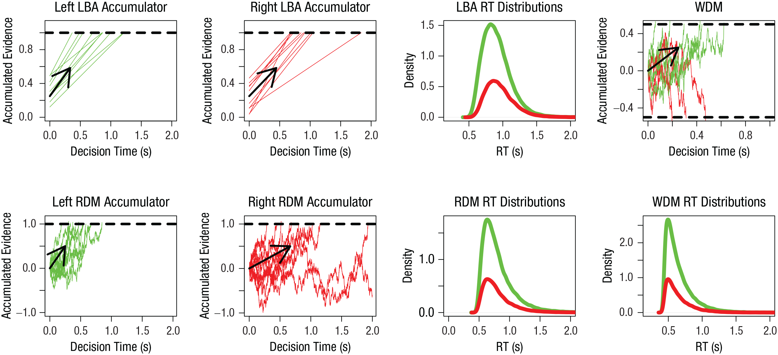
Illustration of a linear ballistic accumulator (LBA), racing diffusion model (RDM), and Wiener diffusion model (WDM) for a choice between “left” and “right” response options when the “left” option is correct (accuracy ~ 73% in all cases). The graphs show the level of accumulated evidence as a function of time and the corresponding response time (RT) distributions for each model. Evidence trajectories and RT distributions for the “left” response are shown in green, and evidence trajectories and RT distributions for the “right” response are shown in red. The LBA and RDM have one accumulator for each response option, each with its own threshold, indicated by a dashed line. For the WDM, there is only one accumulator, but it has two thresholds: The upper dashed line corresponds to the threshold for the “left” response, and the lower dashed line corresponds to the threshold for the “right” response. In all cases, the RT distributions are depicted in their defective form, in which the area under the curve equals the probability of the corresponding response. For each accumulator, evidence trajectories during 10 trials are plotted (straight lines in the LBA, jagged lines in the others); arrows show the average accumulation rates. Each LBA accumulator has independent trial-to-trial variability in the accumulation rate, which has a Gaussian (i.e., normal) distribution, and in the starting point, which has a uniform distribution. Both the RDM and the WDM have Gaussian moment-to-moment variability in their accumulation rates; this variability is independent between the two accumulators in the RDM. R script for the parameters and code to plot this figure are available at OSF, at https://osf.io/xzhe5. The original figure is available under a CC-BY 2.0 license, at https://tinyurl.com/52v7hwam.
In the LBA, accumulation is deterministic (i.e., it occurs at a constant rate within a trial); in the RDM, accumulation is diffusive (i.e., it varies randomly from moment to moment), with a constant average rate. In the LBA, the starting point of accumulation also varies from trial to trial. In both models, the choice is determined by the first accumulator to reach its threshold. Response time (RT) is the sum of decision time (i.e., the time to move from the starting point to the threshold) and nondecision time, typically the sum of the times to encode the choice stimulus and to produce a motor response once a winner is determined. The third column of Figure 2 shows the resulting RT distributions; the area under each distribution represents the corresponding response probability.
The WDM, illustrated in the rightmost column of Figure 2, is a special case of the RDM in which moment-by-moment changes in the level of evidence in one accumulator correspond to equal and opposite changes in the other accumulator. The evidence on which the response is based is thus reduced to a difference between the two accumulators, and the race becomes a tug of war represented as one accumulator with two thresholds. The basic WDM wrongly predicts that incorrect and correct responses have identical RT distributions, so it has been augmented with the same types of trial-to-trial variability as in the LBA, in which case it has been called the diffusion decision model (DDM; Ratcliff & McKoon, 2008). Both the WDM and the DDM remain limited to binary choices, but other diffusive race models, such as the RDM and other variants with less than completely negatively correlated interactions among the runners, are not so limited.
Donkin and Brown (2018) have provided a broad and inclusive review of most types of EAMs. These vary in a variety of ways, such as in whether the accrual of evidence is discrete or continuous and whether it is linear or nonlinear. Bogacz et al. (2007) discussed rationales for the assumptions of EAMs in terms of optimality and their biological basis. Despite the differences among the various types of EAMs, the core parameters are interpreted similarly in all applications: Rates of evidence accrual are determined by arousal, attention, and stimulus characteristics, whereas thresholds are set to strategically control caution and bias in responding. Higher thresholds increase caution, slowing responding but increasing accuracy (i.e., the speed-accuracy trade-off) by overcoming starting-point biases or averaging out diffusive variability. Bias occurs when the threshold is lower for one response than for another.
Figure 3 shows examples of the LBA and RDM used as components in models of complex tasks. Strickland et al.’s (2018) prospective memory decision-control (PMDC) model (see Fig. 3a for details) addresses a prospective memory (PM) task in which participants view a series of letter strings; in most trials, they must indicate whether the string is a word or nonword, but in a small subset of randomly selected trials, the stimulus has an attribute (e.g., the substring “tor”) that requires them to remember to make a different response. To model performance on this task, Strickland et al. augmented a binary-choice LBA with a third accumulator for the PM response. The PMDC model provided a novel cognitive-control-based perspective on PM, illustrating how race models can be used to instantiate both reactive (i.e., stimulus-driven) control, through feedforward inhibition of routine responses when a PM stimulus is detected, and proactive (i.e., anticipatory) control, through setting different thresholds for different accumulators.
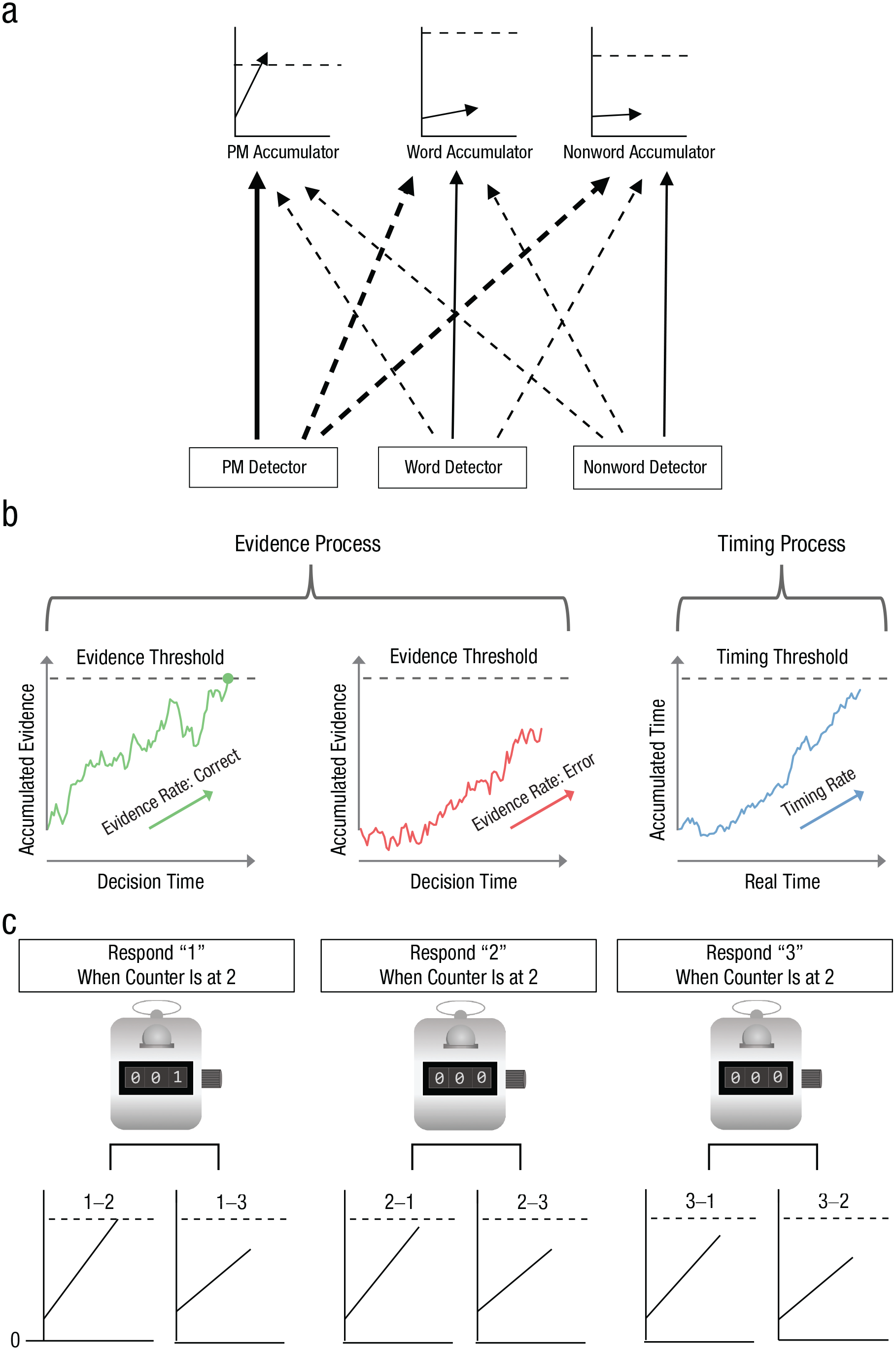
Examples of the linear ballistic accumulator (LBA) and racing diffusion model (RDM) as components in models of complex tasks. Strickland et al.’s (2018) prospective memory decision-control model, illustrated in (a), is a standard binary LBA (i.e., it includes two accumulators corresponding to two response options) that makes a lexical decision (i.e., word vs. nonword) on the basis of inputs from word and nonword detectors unless the accumulators for these responses are beaten by a third, prospective memory (PM) accumulator that receives input from a detector for a PM stimulus attribute (e.g., “tor” as a substring of the lexical decision stimulus). Solid arrows indicate excitatory inputs and dashed lines inhibitory inputs; thicker lines indicate stronger connections. The PM detector both excites the PM accumulator and inhibits the lexical decision accumulators, instantiating reactive control. Similarly, the word detector excites the word accumulator and inhibits the PM and nonword accumulators, and the nonword detector excites the nonword accumulator and inhibits the PM and word accumulators. Response thresholds instantiate proactive inhibition, in this example, favoring PM responses by setting a lower threshold for the PM than for the word accumulator, as only words can contain the PM stimulus. Hawkins and Heathcote’s (2021) timed racing diffusion model, illustrated in (b), is a standard binary RDM (the evidence process) that makes choices in the usual way unless beaten by a third accumulator (the timing process), in which case a random choice is made. Separate accumulators accrue evidence for the correct response and the error response. In this illustration, the green circle marks the point at which the former accumulator won the race. The advantage LBA model developed by van Ravenzwaaij et al. (2020), illustrated in (c), accounts for a choice between three alternatives (labeled “1,” “2,” and “3”; the same approach can be generalized to any number of choices). In this model, standard LBAs accumulate “advantage” evidence (i.e., evidence for one stimulus over another; e.g., 1-2 evidence has a mean equal to the mean for the evidence for Choice 1 minus the mean for the evidence for Choice 2). A counter for each choice starts at zero and is connected to a set of accumulators registering the advantage of that choice over the other options; the counter is incremented each time one of the accumulators reaches its threshold. Under a win-all stopping rule, a response is triggered by the first counter to achieve a count equal to the number of accumulators in the set (e.g., in the model illustrated here, the “1” response is triggered if its counter is the first to register two counts).
Hawkins and Heathcote’s (2021) timed racing diffusion model (TRDM; Fig. 3b) combines a binary-choice RDM with a leading model of time perception (Simen et al., 2016), a diffusive process with a constant input and a threshold set so that it is crossed on average at a target time. Previous attempts to model the effect of the passage of time on decision making relied on implicit timing mechanisms such as decreasing thresholds. The TRDM provides a comprehensive account of such effects with an explicit and hence testable mechanism that is grounded in the literature on timing tasks.
Finally, van Ravenzwaaij et al.’s (2020) advantage LBA (ALBA) models responding contingent on more than one LBA threshold-crossing event. Accumulators correspond to “advantages,” that is, evidence for the presence of one stimulus over another (see Fig. 3c for details). The ALBA accounts for competition effects among choice options previously thought to rule out independent-race models. It extends to cases of more than two response options and predicts Hick’s law, a logarithmic increase in RT as the number of choices increases. The ALBA uses dynamic logical “AND” functions such that all accumulators in a group must finish to trigger a response. Other logical functions can be constructed similarly (e.g., an “OR” function requires only one group member to finish) to provide the building blocks for powerful and general-purpose computations.
Reynolds et al. (2021) proposed an alternative to the ALBA account that requires only two accumulators when there are more than two response options. They built on Vickers’s (1979) hypothesis that equates confidence with a “balance of evidence,” the difference between the winning and losing accumulator when the winner achieves threshold. Reynolds et al. added a set of thresholds to each accumulator to translate the balance of evidence into discrete responses. For example, a choice is rated as uncertain if the losing accumulator has passed all but the last threshold when the winner reaches the threshold (i.e., the loser is not far behind the winner). Figure 4 illustrates this multiple-threshold race (MTR) model and related approaches in which a response is triggered as a function of the states of both accumulators; the response may be based on the total number of thresholds passed, or the thresholds themselves may be defined jointly by both accumulators’ states. Kvam (2019) proposed a geometric perspective integrating these and other race models. In this framework, the state of each accumulator is represented as Cartesian coordinates. Building on Smith’s (2016) seminal circular-diffusion model, Kvam showed that with enough thresholds, or a nonlinear joint threshold, race models can be extended to accommodate continuous responding. Kvam et al. (2022) used this approach to provide a unified account of discrete and continuous responding with respect to line-length and color-matching judgments.
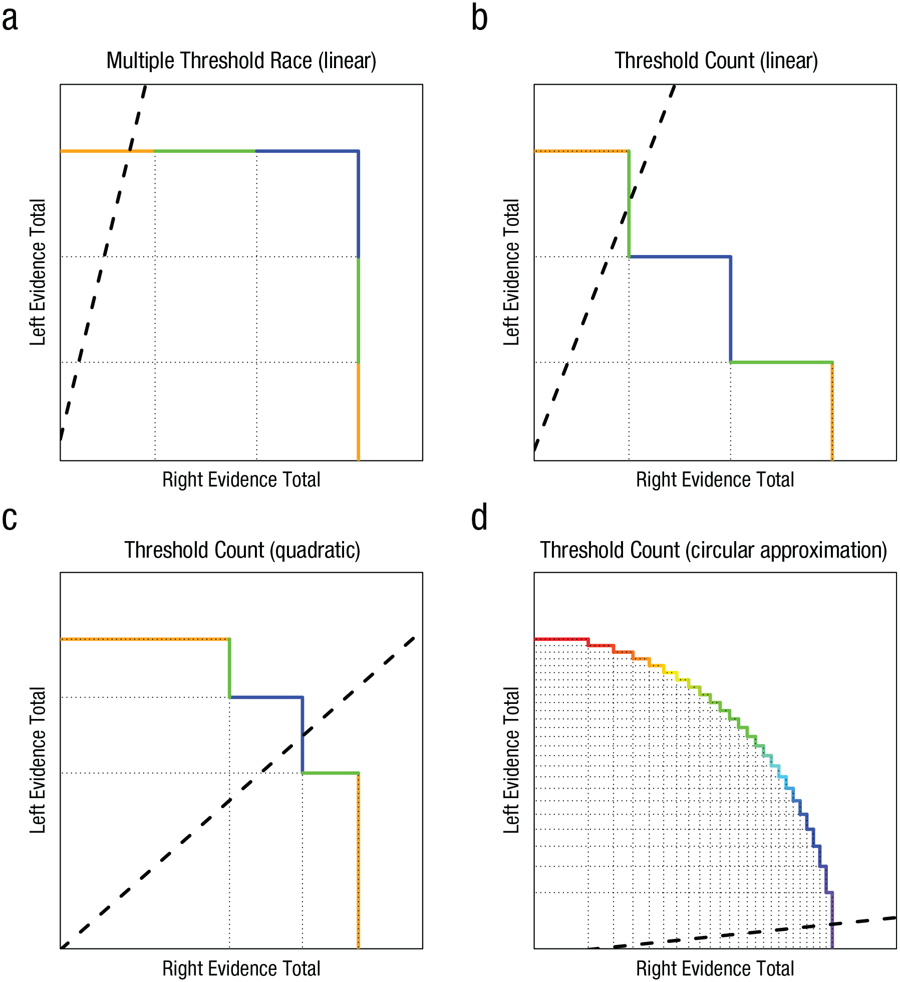
Geometric representations (based on Kvam 2019) showing how two racing accumulators (favoring right vs. left ends of a dimension) account for selection among more than two responses by triggering a response that is based on a particular threshold-crossing event but also contingent on previously occurring threshold-crossing events. For instance, the dimension could range from high confidence in one choice to high confidence in the opposite choice, or from low (e.g., red) to high (e.g., violet) wavelengths of light. The state of the right accumulator is represented on the x-axis, and the state of the left accumulator is represented on the y-axis, so each point on the plane represents the joint state of the two accumulators at a given time. The dashed lines represent examples of how the joint state evolves over time when accumulation is linear and deterministic. Each accumulator has multiple thresholds: Horizontal dotted lines represent thresholds for the left accumulator, and vertical dotted lines represent thresholds for the right accumulator. Each colored line segment corresponds to a different response, which is based on a combination of threshold-crossing events. The four panels represent the relationship between Reynolds et al.’s (2021) multiple-threshold race (MTR) models (a) and threshold-counting models (b–d) within Kvam’s (2019) general geometric framework, in which a response is triggered, and an option chosen, on the basis of the x and y states. The diagram in (a) represents an MTR model in which selecting among six responses is accounted for using three thresholds per accumulator. Responding is triggered the first time an accumulator’s highest threshold is crossed, and the response selected depends on how many of the losing accumulator’s thresholds were previously crossed. This example illustrates a model for a task requiring binary choices (e.g., “left” vs. “right”) rated as being made with low, medium, or high confidence. Orange segments correspond to high-confidence responses, green segments to medium-confidence responses, and blue segments to low-confidence responses; segments on the horizontal line correspond to choosing the “left” response, and segments on the vertical line correspond to choosing the “right” response. In this example, the left accumulator crossed all three thresholds before the right accumulator crossed any, which corresponds to a high-confidence “left” response. Note that the two accumulators could have different numbers of thresholds, thresholds could be spaced unevenly, and different segments could be mapped to the same option. The diagrams in (b), (c), and (d) represent threshold-counting models, alternatives to the MTR models. Threshold-counting models have been used to account for both discrete and continuous responding (Kvam et al., 2022). The diagram in (b) represents a threshold-counting model with three evenly spaced thresholds for each accumulator: A response is triggered when three thresholds have been crossed. This diagram continues the example of the task described for (a). In this case, the first right threshold is crossed after two left thresholds have been crossed, and this triggers a medium-confidence “left” response. The diagram in (c) represents a threshold-counting model that has quadratically spaced thresholds (i.e., even spacing on a squared scale) and accounts for the same responses as in (b). In this case, after the first right threshold is crossed, the first left threshold is crossed, and then a second right threshold is crossed; this triggers a low-confidence “right” response. The diagram in (d) represents a threshold-counting model with 25 quadratically spaced thresholds for choosing a color of the rainbow (a violet choice is illustrated). In the limit of a large number of thresholds, this model approximates a circular boundary in Kvam’s (2019) geometric framework (i.e., a response is triggered when
What Are the Advantages of Using Race Models?
The expressive power of race models is being used in an increasing number of areas. What motivates researchers to quantitatively instantiate their psychological-process theories in this way? One motivation is to avoid mistaken psychological inferences based on data reflecting speed-accuracy trade-offs. For example, Evans et al. (2018) applied the LBA to data from the Human Connectome Project and showed that performance correlations between twins that had been interpreted in terms of cognitive ability were more likely due to the heritability of response caution. Because correctly identifying underlying causes is key for effective interventions, EAMs are increasingly being used in areas ranging from computational psychiatry (e.g., attention-deficit/hyperactivity disorder; Weigard et al., 2018) to performance in time-pressured multitasking environments (e.g., Palada et al., 2019).
EAMs are also used as a second stage, or back end that enables decision-making effects to be disentangled from the effects of an initial stage, or front end, modeling nondecision phenomena. For example, Steyvers et al. (2019) combined a front end accounting for trial-to-trial changes in task-set activation with an LBA back end to model task-switching costs (i.e., slower responding after switching than after repeating tasks). The specificity of this approach supports clearer selection among theoretical positions, and it has been applied, for example, to theories of attentional selection in vision (White et al., 2011), to primacy and recency effects in free recall (Osth & Farrell, 2019), and to theories of multiattribute choice (i.e., choice between options that differ along more than one dimension; Evans et al., 2019). The latter case is instructive regarding the utility of the additional constraint afforded by RTs, as the model that best fit the data differed from earlier comparison models based only on choice data. Incorporating RTs also brings measurement advantages. For example, Jones et al.’s (2015) race model of health-care preferences elicited by identifying the best and worst among a set of options provided the equivalent (in terms of estimation precision) of more than doubling sample size relative to traditional choice-only models. Front ends can also model variability in processing times that adds to a race model’s decision time, such as in Provost and Heathcote’s (2015) model of the mental-rotation-matching task, or can consist of a series of decision stages, as in Fific et al.’s (2010) test of different mental architectures for categorization.
Race models afford even greater expressive ability through probabilistic mixtures that model participants performing a task in different ways on different trials. In work with human participants, mixture models have been used to account for guessing in visual working memory tasks (Donkin et al., 2013) and to misapplication of complicated decision rules (Bushmakin et al., 2017). They have also been used to model monkeys’ low caution in a putatively high-caution condition (Cassey et al., 2014). The ability to test for changes across trials in the cognitive mechanisms determining responses can have applied as well as theoretical implications. For example, we (Matzke et al., 2017) used the mixture approach to account for goal neglect that causes the stop runner to fail to enter the race in response to a stop signal. In our model, the finishing times of the go and stop runners were described by the sum of Gaussian and exponential random variables (i.e., ex-Gaussian distribution). Goal neglect, rather than inhibitory deficits (i.e., slowing of the stop runner), was found to explain why participants with schizophrenia performed more poorly than healthy control participants in the stop-signal task.
How Should Race Models be Used?
Race-model parameters enable insights into the psychological causes of observed phenomena. Going beyond the ability of simple EAMs to account for speed-accuracy trade-offs, the race models in Figure 2 enable insights into more complex constructs. For example, Strickland et al. (2018) found that PMDC parameter estimates indicate that prospective memory failure is mainly due to reactive control rather than proactive control or limited attention capacity.
Race models can also be used to unify theoretical constructs. For example, Hawkins and Heathcote (2021) found that people with greater precision (i.e., less moment-to-moment variability) in the diffusion process underlying a time-interval-production task also had higher precision in the timing component of the TRDM. Reynolds et al. (2020) used the MTR framework to unify race models with perhaps the most widely applied cognitive model, signal detection theory, providing estimates of its discriminability and bias parameters that are informed by RT.
However, to be valid, parameter values must be uniquely identified by the data from which they are inferred. That is not always guaranteed, particularly when the number of observations per participant in each condition is low. We (Heathcote et al., 2019) addressed this issue using hierarchical Bayesian estimation and demonstrated the many advantages of a Bayesian approach. Fitting models to simulated data makes it possible to assess estimation accuracy and precision by comparing the parameters known to generate the data with the parameters that the model infers on the basis of the data. We strongly recommend that such parameter-recovery studies be carried out not only for new models but also for applications of existing models to new designs. If problems emerge, either the design or the model must be adjusted. Hierarchical estimation can help when the number of observations per participant is limited, by constraining each participant’s estimates through a group-level model of individual differences. When there are enough participants, well-estimated group-level parameters can be obtained, although limitations may remain for the participant-level estimates.
Carefully chosen parameterizations are key for both estimation and interpretation. Ideally, accumulation-rate parameters should be made a function of stimulus values. A simple and general way to do so has been proposed by van Ravenzwaaij et al. (2020), who applied it to determine rates (V) when the decision involves choosing the brighter of two stimuli, one on the left (L) and one on the right (R):


Parameter s quantifies cognitive-processing speed, and wS and wD are the weights of the sum (i.e., overall magnitude) and difference (i.e., advantage), respectively, of the subjective brightness of the two stimuli (BL and BR). Subjective brightness followed Weber’s law in being a logarithmic function of the objective luminance. When objective and/or subjective stimulus values are not available, the processing-speed and magnitude terms are not separately identifiable. In traditional EAMs, it can also be useful to interpret differences between the estimated accumulation rates as reflecting the aggregate impact of the discriminability of the stimuli corresponding to different choices and the quality of selective attention to the stimulus features that support that discrimination, and to interpret the sum term as reflecting the aggregate impact of internal (e.g., processing speed) and external (e.g., stimulus magnitude) factors driving a response to occur.
Our final example shows how a single race model can provide a multifaceted characterization of psychological processing that is theoretically revealing, in this case, in the domain of healthy cognitive aging. Slowing with age is pervasive, so leading theories posit a reduction in cognitive-processing speed with age as a broad explanatory factor, but age-related performance decrements have also been attributed to reduced executive function (i.e., reduced ability to flexibly maintain and update goals). We (Heathcote et al., 2022) investigated these theories using a novel stop-signal task (see Fig. 5) requiring inhibition of both easier and harder binary choices, as well as proactive control on go trials based on cues about the response most likely to be correct on the upcoming trial. We fitted a previous stop-signal model (Matzke et al., 2017) with an ex-Gaussian stop runner but replaced the model of the go trials with RDM runners. The hybrid ex-Gaussian/RDM approach provides a rich array of measures, including the key index of inhibitory ability, stop-signal RT, as well as goal neglect and measures based on RDM go processing—peripheral processing speed (nondecision time), central processing speed (average accumulation rate), selective attention (the difference between accumulation rates), caution, and proactive control of bias in response thresholds.
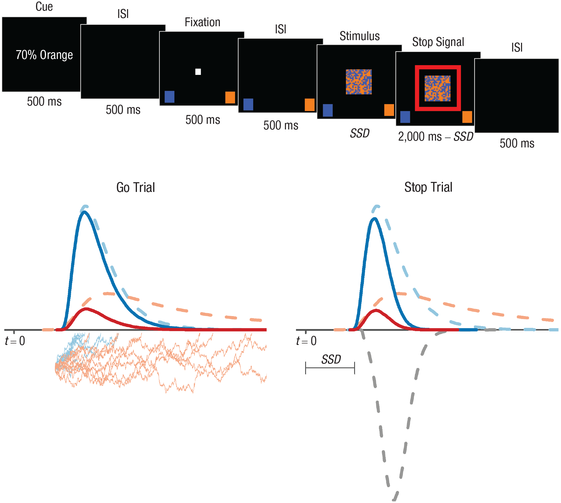
Illustration of a hybrid ex-Gaussian/racing diffusion model applied to a stop-signal task (Heathcote et al., 2022). The go (i.e., choice) stimuli were 20 × 20 grids of blue and orange squares whose position changed randomly on each screen refresh (see https://youtu.be/kXZk_jCHjkM for a video of the task). Participants had to decide which color was dominant. Choice difficulty varied randomly from trial to trial; the dominant color constituted 52% of the squares on harder trials and 54% on easier trials. The top panel illustrates the sequence in a stop trial requiring participants to withhold their response. The cue indicates that there is a 70% chance that orange will be the dominant color in the upcoming stimulus. Stop trials differed from go trials only in that a red square appeared around the choice stimulus at a stop-signal delay (SSD) that increased by 50 ms after a stop trial on which response inhibition was successful (which made stopping more difficult on the next stop trial) and decreased by 50 ms after a stop trial on which response inhibition failed (which made stopping easier on the next stop trial). The stop signal occurred on a randomly ordered 25% of trials. ISI = interstimulus interval. The bottom panel illustrates the go-trial (left) and stop-trial (right) models for this task (t = 0 represents the onset of the choice stimulus). On go trials, once the stimulus is encoded, two runners corresponding to the “orange” and “blue” response options start to race each other from the same initial level. The jagged lines illustrate noisy accumulation of evidence for 10 races. The total that first crosses its response threshold triggers the associated response. In the illustration, the thresholds for the two response options are assumed to be the same and correspond to the x-axis, but when there is response bias, the thresholds for the two accumulators may differ. The dashed lines above the x-axis correspond to the distributions of the two runners’ finishing times across many trials; finishing times are longer for the orange accumulator because it has a lower average accumulation rate. The solid lines correspond to the distributions of the winning times for the two accumulators, which are shorter than the finishing times because faster runners win races. The stop-trial model shows the distributions of the finishing and winning times on stop trials. The finishing time of the stop runner is assumed to have a truncated ex-Gaussian distribution with a lower bound of 50 ms (i.e., the additional gray dashed line below the x-axis). The finishing-time distributions for the go runners are assumed to be identical on stop and go trials. The presentation of the go stimulus is followed at time t = SSD by a stop signal that triggers the stop runner. The go response is successfully inhibited when the stop runner finishes before either of the go runners. Hence, the distributions of winning times for the go runners are faster when inhibition fails (solid lines) than on go trials because slower go finishing times tend to lose out to the stop runner. The original figure is available under a CC-BY 2.0 license, at https://tinyurl.com/y5nmbee8.
Our primary finding was that aging affected mainly processing speed, both central and peripheral, and that only a small part of slowing was due to caution increasing with age (Heathcote et al., 2022). There was no evidence of any age-related deficit in executive-function measures except response inhibition; that deficit was mediated by slowing in the speed of the inhibitory runner. If anything, older participants had less goal neglect, and better selective attention and proactive threshold control. These results are surprising given that Ratcliff and McKoon (2008) summarized the results of almost a dozen applications of the traditional DDM to aging as showing that “the slowdown is almost entirely due to older adults’ conservativeness [i.e., caution]” (p. 911). One explanation is that, in being driven purely by the difference in evidence between two options, the DDM is unable to represent effects of stimulus magnitude and central processing speed, and so any reduction to the latter in older participants can be attributed only to increased caution. A more recent revision of the DDM can account for stimulus magnitude with the additional assumption that the mean and variability of accumulation rates are positively related (Ratcliff et al., 2018). Further research will be required to determine what this new type of DDM indicates about the causes of age-related slowing.
These results not only show how race models can provide theoretical insights, but also highlight the challenges with respect to parameter estimation and interpretability. First, the descriptive ex-Gaussian account of the stop runner (Matzke et al., 2017) had to be retained in our hybrid model (Heathcote et al., 2022) because stop-signal models in which all runners are evidence-accumulation processes result in extremely poor parameter recovery (Matzke et al., 2020). In contrast, the hybrid model’s parameters are well recovered, even in our complex design, the key factor being that the ex-Gaussian account does not require the estimation of the nondecision time of the stop runner. Second, the strong theoretical divergence between the DDM and the hybrid model underlines the need to carefully consider the limitations in what a model can and cannot represent, and the potential for parameter trade-offs, when interpreting any model-based estimate.
Future Directions
A range of emerging applications are using race models to integrate different data sources, tasks, and theoretical frameworks. For example, the LBA has been used to simultaneously link behavioral data to functional MRI and electroencephalograph data through hierarchical Bayesian estimation (Turner et al., 2016). Similar methods have been used to link performance in multiple tasks through shared LBA parameters (Wall et al., 2021). We believe that these joint models are more likely to be successful at linking data of different types and from different tasks than are approaches, such as structural equation modeling, that ignore the details of cognitive processing or implicitly assume details, which are explicit (and hence testable) in joint models.
Miletić et al. (2021) generalized and improved on previous attempts to integrate another very successful type of cognitive model, reinforcement-learning models, into the race-model framework. They used a simple learning rule that allowed the model to learn reward values for stimuli on the basis of probabilistic feedback from forced choices. These values played the role of brightness in van Ravenzwaaij et al.’s (2020) equations, determining rates for RDM accumulators. The results of the model agreed with van Ravenzwaaij et al.’s results for perceptual choice: The learned values affected accumulation rates mainly through the advantage term, but the magnitude term also played a nonnegligible role. In binary-choice tasks, the model outperformed previous approaches that combined the DDM with reinforcement learning; further the model went beyond what can be achieved with the DDM, successfully addressing a three-choice task and reward-magnitude effects.
In closing, we note that most of the race models discussed here have been analytically tractable enough to yield an easily computed likelihood, the key quantity required for fitting the models to data in a comprehensive way. However, requiring such tractability can limit the scope of potential applications. Fortunately, recent developments in approximate-likelihood methods, combined with faster hardware (Lin et al., 2019) and deep neural network approaches to Bayesian estimation (Radev et al., 2020), look set to make it increasingly practical to employ race models in a wider range of applications.
Recommended Reading
Donkin, C., & Brown, S. D. (2018). (See References). A broad and integrative historical overview of evidence-accumulation models, their applications (from measuring latent constructs to developing theory in cognitive science and neuroscience), and methods for estimation, evaluation, and inference with respect to these models.
Heathcote, A., Lin, Y.-S., Reynolds, A., Strickland, L., Gretton, M., & Matzke, D. (2019). (See References). A practical introduction to estimation and inference for a variety of race models implementing hierarchical Bayesian Markov chain Monte Carlo sampling in a collection of functions, with associated tutorials in the R language.
Kvam, P. D. (2019). (See References). A more advanced reading (and winner of the 2021 R. Duncan Luce Outstanding Paper Award from the Society for Mathematical Psychology) providing a novel perspective on both deterministic and stochastic race models, placing them in an integrative geometric framework that encompasses both discrete and continuous responding.
Miletić, S., Boag, R. J., Trutti, A. C., Stevenson, N., Forstmann, B. U., & Heathcote, A. (2021). (See References). An evaluation of how well the diffusion decision model and a variety of racing diffusion models integrate with simple reinforcement learning, finding that input equations and architectures from van Ravenzwaaij et al.’s (2020) “advantage” framework provide the best account of learning in value-based decision making.