Probabilistic Biases Meet the Bayesian Brain

Abstract

In Bayesian cognitive science, the mind is seen as a spectacular probabilistic-inference machine. But judgment and decision-making (JDM) researchers have spent half a century uncovering how dramatically and systematically people depart from rational norms. In this article, we outline recent research that opens up the possibility of an unexpected reconciliation. The key hypothesis is that the brain neither represents nor calculates with probabilities but approximates probabilistic calculations by drawing samples from memory or mental simulation. Sampling models diverge from perfect probabilistic calculations in ways that capture many classic JDM findings, which offers the hope of an integrated explanation of classic heuristics and biases, including availability, representativeness, and anchoring and adjustment.

Human probabilistic reasoning gets bad press. Decades of brilliant experiments, most notably by Daniel Kahneman and Amos Tversky (e.g., Kahneman, 2011; Kahneman, Slovic, & Tversky, 1982), have shown a plethora of ways in which people get into a terrible muddle when wondering how probable things are. Every psychologist has learned about anchoring, conservatism, the representativeness heuristic, and many other ways that people reveal their probabilistic incompetence. Creating probability theory in the first place was incredibly challenging, exercising great mathematical minds over several centuries (Hacking, 1990). Probabilistic reasoning is hard, and perhaps it should not be surprising that people often do it badly. This view is the starting point for the whole field of judgment and decision-making (JDM) and its cousin, behavioral economics.

Oddly, though, human probabilistic reasoning equally often gets good press. Indeed, many psychologists, neuroscientists, and artificial-intelligence researchers believe that probabilistic reasoning is, in fact, the secret of human intelligence. Indeed, one particularly important element of probability, Bayes’s theorem, has come to name an entire subfield: Bayesian cognitive science (e.g., Tenenbaum, Kemp, Griffiths, & Goodman, 2011), spawning probabilistic models of perception (Kersten, Mamassian, & Yuille, 2004), categorization (Anderson, 1991; Lake, Salakhutdinov, & Tenenbaum, 2015; Sanborn, Griffiths, & Navarro, 2010), reasoning and argumentation (Hahn & Oaksford, 2007; Oaksford & Chater, 1994, 2020), and intuitive physics (Battaglia, Hamrick, & Tenenbaum, 2013; Sanborn, Mansinghka, & Griffiths, 2013). In parallel, neuroscientists have conceived of the brain as a Bayesian inference machine (Doya, Ishii, Pouget, & Rao, 2007). Bayesian methods are also widespread beyond psychology—from economics (Karni, 2011) to philosophy of science (Howson & Urbach, 2006).

What is going on? How can two of the most important and influential research programs in psychology be built on entirely contradictory assumptions? If the human mind is a spectacularly powerful probabilistic-inference machine, why do people fall into systematic and elementary probabilistic errors?

There are various approaches to resolving this puzzle (Oaksford & Chater, 2007). For example, we might propose that low-level, modular, repetitive processes (vision, motor, language processing) are Bayesian but that high-level, effortful, general-purpose, central cognitive processes are not. Alternatively, or additionally, we might suspect that the Bayesian brain operates only on data gathered by the senses and cannot deal with explicit probability problems formulated in words or symbols.

We are sympathetic to these viewpoints but note that when performance is measured in the same way, there is surprising similarity between low-level and high-level processes (Jarvstad, Hahn, Rushton, & Warren, 2013). But is there a more direct approach? The Bayesian account of cognition cannot be taken literally, even when it is most successful. For example, a literal Bayesian approach to vision would require calculating the myriad probabilities of each possible layout of the environment, given a particular visual input, by applying Bayes’s theorem. But these calculations are astronomically complex. So Bayesian computational models, and presumably the brain itself, can only be approximating optimal Bayesian calculations: For complex real-world problems, human rationality can only be bounded (i.e., restricted by computational constraints, Gigerenzer & Selten, 2002; Lieder & Griffiths, 2020; Simon, 1955; and perhaps using heuristics corresponds to Bayesian inference with extreme priors, Parpart, Jones, & Love, 2018).

Any approximation will, inevitably, generate mistakes—this is what makes it an approximation after all. Reconciliation of JDM research and Bayesian cognition would be possible if the way the brain approximates Bayesian calculations generates the very errors and biases that JDM research has uncovered.

A very natural and simple way of approximating Bayesian calculations, and one that is widely used in computational statistics and machine learning (so-called Monte Carlo methods), maps naturally onto the parallel hardware of the brain (Buesing, Bill, Nessler, & Maass, 2011; Orbán, Berkes, Fiser, & Lengyel, 2016) and builds on well-established psychological processes of memory retrieval and mental simulation. Rather than attempting implausibly complex mathematical calculations using the laws of probability, the brain needs only to sample from a model of some aspect of the world (Bonawitz, Denison, Griffiths, & Gopnik, 2014; Griffiths, Vul, & Sanborn, 2012; Sanborn & Chater, 2016)—and, often, sampling is easy, even if Bayesian probability calculations are incredibly hard. If the brain could sample forever, then, in certain circumstances, the frequencies of the sample will come to match the “true” probabilities arbitrarily accurately. But, in reality, the size of the sample might be very small—perhaps even just one instance in some cases (Vul, Goodman, Griffiths, & Tenenbaum, 2014). Hence, the sample will give only a rough clue about the “correct” probabilities—but still this clue may be enough to help the brain make “good enough” decisions. The results of the sample can then be converted into choices or judgments. Indeed, assuming a small sample that is then converted either into estimates of probability or into confidence intervals has successfully explained how overconfidence effects strongly depend on how participants are asked to respond (Juslin, Winman, & Hansson, 2007).

Deriving probabilities from frequencies drawn from samples is reminiscent of, but very different from, the frequentist interpretation of probability familiar from classical statistics and associated with Fisher and Neyman (Hacking, 1990). Whereas Bayesians interpret probabilities as subjective degrees of belief of a particular agent or person, frequentists aim for a more “objective” interpretation of probability in terms of limiting frequencies of repeated experiments in the external world (e.g., flipping a coin), which is independent of the individual. Sampling models in cognitive science are inherently tied to the psychology of the individual, depending on the individual’s probabilistic model from which the sample is drawn—thus, different agents with different internal models (or items retrieved from memory) will assign different probabilities to the same event. Thus, although sampling models involve frequencies, these frequencies approximate the subjective probabilities familiar to Bayesians, particularly those of unique events; these models do not embody a frequentist interpretation of probability.

There is, however, an important distinction between cognitive models that apply “raw” relative frequencies, based on a mental sample (e.g., Costello & Watts, 2014), and those that take a Bayesian approach a step further (e.g., Zhu, Sanborn, & Chater, 2020) by integrating samples with background knowledge (in the spirit of Bayesian Monte Carlo in machine learning; Rasmussen & Ghahramani, 2003). This difference is especially important when sample sizes are small. But before exploring the distinctions between sampling models, we will first make broader comparisons between sampling and the heuristics-and-biases literature.

Rethinking Probabilistic Irrationality: From the Matching Law to Heuristics and Biases

The sampling viewpoint predicts a variety of recalcitrant patterns of apparently irrational behavior. Consider probability matching: the tendency for people to predict the next item in a sequence in proportion to its probability rather than always picking the most probable next item (e.g., Koehler & James, 2009). Suppose the true probability of heads is two thirds and tails is one third. Always choosing the most probable option (heads) will be correct with probability 2 out of 3. But matching, that is, predicting heads two thirds of the time and tails one third of the time, will be correct with probability (2/3 × 2/3) + (1/3 × 1/3) = 5/9. Several authors have pointed out (e.g., Vul et al., 2014) that, although suboptimal, matching makes sense if we assume that people draw a single sample and simply follow that prediction.

A second consequence is that people will overestimate items that are readily available in memory or easy to mentally simulate. Tversky and Kahneman (1973) found that words beginning with k are judged to be more frequent than words with k as the third letter, although they are much less common—because the first letter provides a much stronger retrieval cue, as would be expected from models of lexical access (e.g., Marslen-Wilson & Tyler, 1980). They also showed that when participants judge the number of paths through a maze, their judgments are strongly influenced by how easily the paths can be found (i.e., sampled through mental simulation). From this present viewpoint, Tversky and Kahneman’s “availability heuristic” is not a specific type of shortcut but a side effect of sampling.

Suppose we want to estimate whether HHHHHH or THTHHHT has the greater probability of being generated by a fair coin flip. If we could draw, say, a few thousand samples, we would conclude that the sequence of length six, HHHHHH, has a relative frequency of about (1/2)⁶ = 1/64 and that the sequence of length seven, THTHHHT, has a relative frequency of about (1/2)⁷ = 1/128. But if we draw a few samples (e.g., of different lengths), it is unlikely that either sequence will be reproduced exactly. This type of problem can be addressed by so-called approximate Bayesian computation (ABC; Beaumont, 2019), used for real-world problems (e.g., with speech waves or images) in which the chance of sampling an exact match with the data is close to nil. ABC counts up samples that are close enough to the data according to some similarity measure. Assuming that one unstructured mix of heads and tails is judged to be similar to another (irrespective of sequence length) and very dissimilar from a “pure” sequence of heads, we would find that many more samples are similar to THTHHHT than HHHHHH, leading to the erroneous conclusion that the first sequence is more probable. Thus, sampling, combined with independently testable assumptions about similarity, provides a novel explanation of the origin of the representativeness heuristic (Kahneman & Tversky, 1972): that the probability of an item is judged by its similarity with respect to a category samples (whether lawyers or engineers, or sequences of random coin flips). Again, according to the sampling viewpoint, representativeness operates not as a specific mental shortcut (i.e., the representativeness heuristic) but as a side effect of judging probabilities by drawing mental samples to a “tolerance” based on similarity. Of course, this approach depends on psychological assumptions about similarity—but these can be independently evaluated.

So far, we have ignored a crucial aspect of sampling: Often one cannot easily draw independent samples from one’s probability distribution—but it is possible to draw a stream of samples, each of which is a variant on the last. Under certain conditions, then, if one samples long enough, one can fill out the whole probability distribution because the stream of samples gradually explores the whole distribution—and this is the justification for the method, known as Markov chain Monte Carlo (MCMC), invented at Los Alamos laboratories (Metropolis, Rosenbluth, Rosenbluth, Teller, & Teller, 1953). MCMC is now a workhorse of Bayesian computational models, including models of cognition—but it is also a psychologically natural hypothesis. After all, peoples’ memories and imaginations operate mostly by small “jumps” (Hills, Jones, & Todd, 2012)—retrieving or simulating a specific item tends to “prime” psychologically similar items (this point is also captured in non-Bayesian sampling models; Costello & Watts, 2018).

Dasgupta, Schulz, and Gershman (2017) noted that if the brain uses small correlated samples, as generated by MCMC, then the resulting probability judgments will be powerfully affected by the starting point. Suppose a person wonders what proportion of animal species live in Africa. If the person is prompted to begin with lion, then the next few samples might be the associatively related zebra, antelope, giraffe, and hippopotamus, all of which happen also to live in Africa, thus biasing the person’s estimate upward. If, by contrast, the person begins with squirrel or polar bear, the sample, and hence the person’s estimate, might be very different. All these effects would disappear if a person sampled forever—the person would rove about the entire representational space of animals eventually. But judgments need to be made quickly, from manageable, small samples.

Such effects of starting point of mental sampling can explain a wide variety of nuanced effects, including otherwise puzzling “unpacking effects” (e.g., Sloman, Rottenstreich, Wisniewski, Hadjichristidis, & Fox, 2004). For example, when people judge the probability of an event represented as a list of disjunctions of typical instances, this probability is inflated. For example, the probability of food poisoning, stomach flu, or any other gastrointestinal disease is judged to be higher than the probability of the logically equivalent gastrointestinal disease. But when the disjuncts are atypical, the opposite effect arises. Thus, the probability of gastroenteritis, stomach cancer, or any other gastrointestinal disease is judged to be lower than the probability of the single, logically equivalent, category of gastrointestinal disease. The intuitive insight behind Dasgupta et al.’s (2017) model is that priming the sampling process with typical examples will help people generate or recall examples of the category by starting the search process in parts of the search space with a high proportion of category members. But priming the sampling process with atypical examples will hinder the generation of examples by starting the search process in parts of the space with a lower proportion of category members.

Dasgupta et al. (2017) and Lieder, Griffiths, Huys, and Goodman (2018) also demonstrated that this process leads to yet another of Tversky and Kahneman’s (1974) celebrated heuristics, anchoring and adjustment: that judgments are biased in the direction of a suggested starting point. For example, in estimating the number of countries in the United Nations, a person will draw samples from a probability distribution over possible values but will be biased by the starting point suggested by an anchor number, even when that anchor has been generated by a random process (e.g., a roulette wheel) and is clearly objectively irrelevant.

The heuristics-and-biases program captures a broad range of phenomena in a set of distinct heuristics. In the Bayesian sampling approach, by contrast, the aim is to explain these phenomena as arising from different aspects of a single process: accumulating and drawing conclusions from samples (whether from memory or an internal model). So, for example, the availability heuristic arises directly from some samples being more accessible than others; anchoring arises from the local, correlated nature of sampling; and the representativeness heuristic arises from the fact that people can typically expect to draw only samples that are similar, not identical, to a given outcome. But the sampling approach also has distinctive implications, such as (a) that averaging repeated estimates by a single person should outperform any single best guess because people are repeatedly sampling from their own belief distribution (as shown by Vul & Pashler, 2008) and (b) that these biases will disappear if people are given the time and motivation necessary to draw a large enough sample.

Probability Judgment by Sampling

A particularly direct test of the Bayesian sampling approach is to ask how well it captures people’s explicit probability estimates. Our starting point is an important (but non-Bayesian) sampling model by Costello and Watts (2014), which provides an excellent fit to a variety of results. Costello and Watts began with the assumption that people draw samples, from memory or other sources, and read off probabilities from the frequencies of different outcomes. But, crucially, they suggested that the sampling process is imperfect. Thus, trying to estimate how likely it is to snow on Christmas day, one may misremember some snowy Christmases as snow free, and the reverse. This mechanism produces a simple mechanism for explaining why small probabilities tend to be overestimated, for example. Suppose the probability of Christmas snow is 10% and suppose that a person happens to sample one snowy and nine nonsnowy days from memory. But if, say, 20% of days are misremembered, then it is likely that about two of the nonsnowy days may be recalled as snowy, thus boosting the estimated amount of snow. The effect reverses when one estimates highly probable events, such as nonsnowy days. Thus, Costello and Watts explain the widely observed tendency for probability estimates to be pulled away from the extreme values (e.g., Erev & Wallsten, 1993).

Psychologists have, of course, proposed many other possible explanations for aversion to extreme probabilities. Prospect theory, for example, assumes that decision weights are transformations of explicitly presented probabilities that demonstrate aversion to extremes (Kahneman & Tversky, 1979), and there are other approaches that also assume that noisy processing produces aversion to extreme probabilities (e.g., Erev, Wallsten, & Budescu, 1994; Hilbert, 2012). Costello and Watts (2014) noted that their sampling approach forces judgment biases to be symmetric because the chance that a sample is misrecalled is the same for any event. So if one’s misrecalled sample tends to overestimate snowy days, it would also underestimate nonsnowy days to just the same degree. Extending this line of thinking, Costello and Watts (2014) created a list of probabilistic “identities” over pairs of events, some of which have been shown to match human judgment data surprisingly well and others from which the human data substantially deviate. These reliable matches and mismatches between human judgment and probability theory form a challenge to nonsampling models of probability distortion; Costello and Watts (2014, 2016, 2018) have shown how a sampling model captures both the distortions and the patterns in human probability judgments—demonstrating that these judgments are, as they put it, “surprisingly rational” after all and that irrational judgments are the result of noise.

Zhu et al. (2020) showed that a number of identical mean predictions can be derived from an even more “rational” model, the Bayesian sampler. Zhu et al.’s starting point is that with small samples, reading off relative frequencies cannot be quite right. To illustrate, with a single sample, every event would have a probability of 1 (i.e., 1 out of 1) or 0 (0 out of 1). Instead, we need to moderate these extremes by combining them with reasonable prior assumptions—treating the sample itself as data (as in Bayesian Monte Carlo; Rasmussen & Ghahramani, 2003) that should update prior assumptions. The effects of the prior are substantial for small samples, but like the effects of starting point or autocorrelation discussed above, disappear for large samples. The natural Bayesian calculation here is extremely simple (linearly pulling probabilities away from the extremes) and perfectly mimics Costello and Watts’s (2014, 2016) mean predictions. It is more “rational” because the deviations from probability theory result from using this prior to improve probability estimates based on a small number of samples. Zhu et al. showed that the Bayesian sampler has distinctive predictions for conditional probabilities in which events are correlated (e.g., P(icy | frosty), where samples of frosty days will typically also be icy; see Fig. 1). This is because the Bayesian sampler directly samples from conditional probabilities rather than constructing conditional probabilities from samples, and their empirical data support the Bayesian sampler model.

Fig. 1.

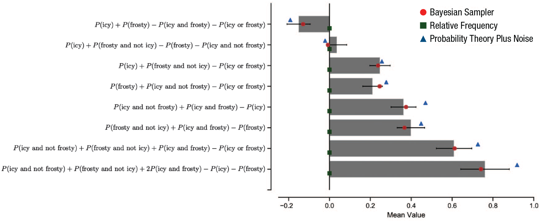
Experimental data and model predictions for probabilistic identities of icy and frosty weather events. Participants were asked to judge individual weather events in a random order, responding to questions of the form, “What is the probability that the weather will be [event X] on a random day in England?” Their weather-probability estimates, labeled “P(event X),” were then combined into probabilistic identities whose calculations are shown along the y-axis. The expected values of identities are shown in bars with 95% confidence intervals across participants. Probability theory predicts that the expected value for each identity should be 0. The overlaid dots are best-fitting-model predictions for three models (green squares: a baseline relative-frequency model, i.e., simply the proportion of samples with a particular property; blue triangles: the probability-theory-plus-noise model, developed by Costello and Watts, 2014, 2016; red dots: the Bayesian sampler). This figure is adapted from Zhu, Sanborn, and Chater (2020).

Another source of potential differentiation between the models concerns the reporting of extreme probability values. Assuming sample sizes are reasonably small, Costello and Watts’s (2014, 2016) model predicts that all samples will or will not be instances of the event of interest—so that probabilities of 0 and 1 will be reported. The Bayesian sampler, by contrast, assumes that all probability judgments will be shrunk by Bayesian correction, so that 0 and 1 values should not be reported except through occasional response error or when generated through reasoning rather than sampling (e.g., if judging P(A or not A), which is clearly 1 through logical analysis alone). Exploring the prevalence of 0/1 probability judgments is therefore a promising direction for future research to distinguish between these sampling models.

The Prospect of Reconciliation?

The development of sampling models as psychological hypotheses provides a possible reconciliation between two apparently diametrically opposed traditions in psychology and neighboring disciplines. Perhaps the rational models of Bayesian cognitive science and the apparently nonrational findings of JDM research arise from a single source: a probabilistic mind based on sampling. If this is right, then both of these important research traditions may benefit from closer interaction. Data from JDM research, behavioral economics, and the gamut of apparent errors and biases across cognitive and social psychology might turn out not to undermine rational models but rather to provide crucial insights into how Bayesian probabilistic calculations are approximated by the brain. Moreover, a Bayesian sampling framework may provide a unified and integrated perspective for apparently unrelated heuristics and biases. It is too early to say how broad and deep such unification might be. But we suggest that initial indications are sufficiently promising to suggest that the possibility of reconciliation should surely actively be explored.

Recommended Reading

Costello, F., & Watts, P. (2014). (See References). Outlines a sampling-based theory of probability judgment in which samples are sometimes misclassified, leading to systematic biases.

Dasgupta, I., Schulz, E., & Gershman, S. J. (2017). (See References). Shows how starting points matter in cognitive models drawing small, correlated samples from memory.

Fiedler, K. (2000). Beware of samples! A cognitive-ecological sampling approach to judgment biases. Psychological Review, 107, 659–676. Shows how the way in which samples are gathered generate a wide variety of often counterintuitive biases in judgment decision-making and social psychology.

Kahneman, D. (2011). (See References). A readable and authoritative introduction to judgment and decisionmaking research from one of its pioneers.

Sanborn, A. N., & Chater, N. (2016). (See References). Proposes that the “Bayesian brain” operates by sampling rather than probabilistic calculation.

Tenenbaum, J. B., Kemp, C., Griffiths, T. L., & Goodman, N. D. (2011). (See References). Outlines a Bayesian approach to human learning and cognition.