
Abstract
An aspect of interest in surveillance of diseases is whether the survival time distribution changes over time. By following data in health registries over time, this can be monitored, either in real time or retrospectively. With relevant risk factors registered, these can be taken into account in the monitoring as well. A challenge in monitoring survival times based on registry data is that the information related to cause of death might either be missing or uncertain. To quantify the burden of disease in such cases, relative survival methods can be used, where the total hazard is modelled as the population hazard plus the excess hazard due to the disease.
We propose a cumulative sum (CUSUM) procedure for monitoring for changes in the survival time distribution in cases where the use of excess hazard models is relevant. The CUSUM chart is based on a survival log-likelihood ratio and extends previously suggested methods for monitoring of time to event data to the excess hazard setting. The procedure takes into account changes in the population risk over time, as well as changes in the excess hazard which is explained by observed covariates. Properties, challenges and an application to cancer registry data will be presented.
Keywords
Introduction
In health registries, such as cancer registries, patients are routinely registered with key disease related and demographic data at diagnosis of disease, and outcome data like survival times are usually added later depending on the characteristics and clinical course of the key disease. Based on such data, an aspect of interest could be to monitor whether the distribution of the time to an outcome of interest changes over time, for instance if the survival times of cancer patients due to the disease itself change over time while adjusting for known prognostic factors. Such monitoring could be of interest both for real-time monitoring of incoming data and for retrospective analyses to pinpoint when in time important changes took place. This could be of value both to monitor for unexpected changes and to monitor if changes in treatment policies can be associated with better outcomes, for example survival benefit for cancer patients.
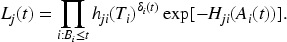
A common challenge in monitoring survival times based on such registry data is that time to death, but not necessarily cause of death, is registered. In addition, even if this information is available, it is often unreliable at population level. Therefore, to quantify the burden of disease in such cases, relative survival methods can be used. Under this framework, the frequent standard assumption is that the total hazard is modelled as the population hazard plus the excess hazard due to the disease, see for example Dickman et al., 1 Perme et al. 2 and Perme et al. 3 for an overview of notions in relative survival and regression models regarding this topic. The population hazard is usually retrieved from national population life tables, stratified on demographic variables.
Methods from statistical process control have been essential in many different fields and applications, originally suggested for monitoring processes in various industries. One of the most widely used control charts is the CUSUM (cumulative sum) presented by Page. 4 Compared to other charts, for example Shewhart charts, the CUSUM chart is known to perform better for detecting smaller shifts that are persistent over time, thus being suitable for a range of medical settings. Over the years, extensions and adaptions of CUSUM charts to a number of different scenarios have been developed. CUSUM procedures for monitoring of ordinary time to event data were first proposed by Biswas and Kalbfleisch, 5 Sego et al., 6 Gandy et al. 7 and Steiner and Jones. 8 These have since been extended to contexts like frailty models,9,10 cure models, 11 illness-death models 12 and queue models. 13 Impact of estimation error in time to event data monitoring was studied by Zhang et al. 14 and effectiveness versus periodic evaluations was studied by Massarweh et al. 15 Applications have been demonstrated in, for instance, monitoring of perioperative mortality.16,17
We propose a CUSUM procedure for monitoring for changes in the time to event distribution when the use of excess hazard models is relevant, for example for monitoring based on registry data with uncertain or missing cause of death information, a typical example being cancer registry data. The CUSUM chart is based on a survival log-likelihood ratio and extends the literature discussed above on monitoring of time to event to the relative survival setting. The procedure takes into account changes in the population risk over time, as well as changes in the excess hazard which are explained by observed covariates. Properties, challenges and an application to cancer registry data will be presented.
The structure of the paper is as follows: Section 2 introduces the set-up and notation and presents the proposed method. In Section 3, numerical simulations and experiments are carried out to demonstrate the use of the method and how it performs under different scenarios, including studying the impact of estimation error. An application of the method on a real data set obtained from the Norwegian Cancer Registry is illustrated in Section 4. Finally, Section 5 provides some concluding remarks. R-code implementing the proposed methods and for running the simulations in Section 3 can be found at https://github.com/jihut/cusum_relative_survival_simulations.
CUSUM chart based on excess hazard models in relative survival setting
Set-up and notation
The setting considered is monitoring time to event under the assumption of an additive hazard model
For ease of notation, consider a monitoring system starting from a given calendar date which is now defined as the origin time point
Further, denote
Let
The proposed CUSUM procedure
Following Gandy et al.,
7
we define a new continuous time CUSUM procedure for the setting of relative survival based on the survival likelihood ratio. Moustakides
18
has shown optimality properties for CUSUMs based on likelihood ratios. The (partial) likelihood
19
based on
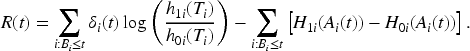

What differs from the procedure in Gandy et al.
7
is that we here work with an excess hazard model and are interested in the change of
In this section, we consider different alternative models for the out-of-control hazard

The proportional alternative implies assuming a larger change in absolute value of the hazard for patients with a higher hazard. However, this might not always be reasonable, and an alternative model for the change could be an additive model where the hazard changes by the same absolute amount for all patients. This motivates an additive out-of-control alternative for the excess hazard. Assuming that we work with non-negative excess hazard, which is usually the case when dealing with cancer patients, the additive alternative is given as

Further, similar to what is considered in Gandy et al.
7
for ordinary survival models, time-transformation alternatives can be used to model changes in the hazard. This is for instance done in order to incorporate more general changes that depend on the definition of the hazard function, for example non-proportional change between the in-control and out-of-control hazard. We consider the following linear accelerated time alternative specified as

A possible challenge with the linear accelerated time alternative occurs if the monitoring system is used to monitor survival up to a certain time point, for instance 10-year survival, and a
Another type of out-of-control models that could in principle be used is models allowing for different changes depending on the value of some of the covariates. For proportional alternatives, this might for instance be an out-of-control model of the form
A final note is that one needs to choose a value of
The signal threshold
Gandy et al.
7
explored the setting of choosing
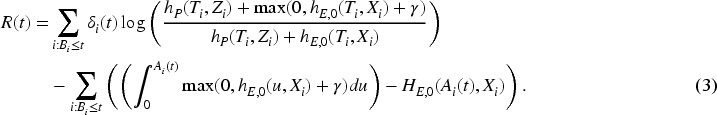
Simulating the signal threshold
Motivated by the preceding section, we opt for the standard strategy of simulating the threshold so that a desired value of the false signal probability (in-control hitting probability) is achieved. In Algorithm 1, an overview of the general approach to simulate the threshold
We will consider two different scenarios for simulating the covariates
Monitoring and updating schemes
The proposed method is best suited for detecting changes in the setting where all observations in the system will experience the out-of-control hazard whenever
With the definition
Although the current method works for real-time monitoring, it is often the case that observations are not registered immediately, and modifications related to the definition of the at-risk time are needed to alleviate this problem. Adjustments to the procedure for various information arrival scenarios are discussed in the following.
For instance, a scenario could be that information about each case becomes available only after censoring or an event. For this setting, Gandy et al.
7
suggested to redefine 
Another circumstance that could appear is when the information is only available at certain time points. An example is when a patient is diagnosed in the middle of a year, but the observation is only included in the database at the end of the year. A possible solution is to again redefine 
Similar to the above, we can extend the first situation where the information of an observation is only available periodically after the observation experiences an event or has been censored, for example when a patient either dies or drops out of a study in the middle of a year and the database is updated with the given observation at the start of the new year. Then, 
Another scenario is when the entire database is updated in regular intervals, adding all information accumulating since the last update. Then, an option would be to run the CUSUM retrospectively by running the CUSUM for the last period once the data for that period become available. This would of course lead to a certain delay in signalling versus when running the chart in real time. Overall, the limitations are not related to the method, but rather the data registrations process. If observations cannot be included in real time, the method can be modified to accommodate this scenario, although that implies that one does not have the trait of real-time monitoring.
In some cases, it is of interest to just monitor for the excess hazard related to survival up to a certain time after diagnosis
Estimating the in-control model
In practical applications, the true in-control excess hazard will be unknown and has to be estimated from baseline data. To run the monitoring procedure, we need to be able to evaluate
When estimating the in-control excess hazard, the estimation error will propagate to the achieved in-control performance. The impact of this, as well as the impact of model misspecifications, will be illustrated in Section 3.5.
Simulation study
In this section, properties of the suggested procedures are studied by simulations.
Simulation set-up
For the following, we will use a proportional excess hazard model, that is
The monitoring is run for 10 years (in one case 5 years) and is using the population hazard of Norway from the beginning of 2010 to the end of 2019. The baseline excess hazard is chosen to be a piecewise constant function of the form
In most simulations, we assume that both the distributions of the covariates and the parameter vectors
The arrival of patients is simulated as a homogeneous Poisson process with an arrival rate
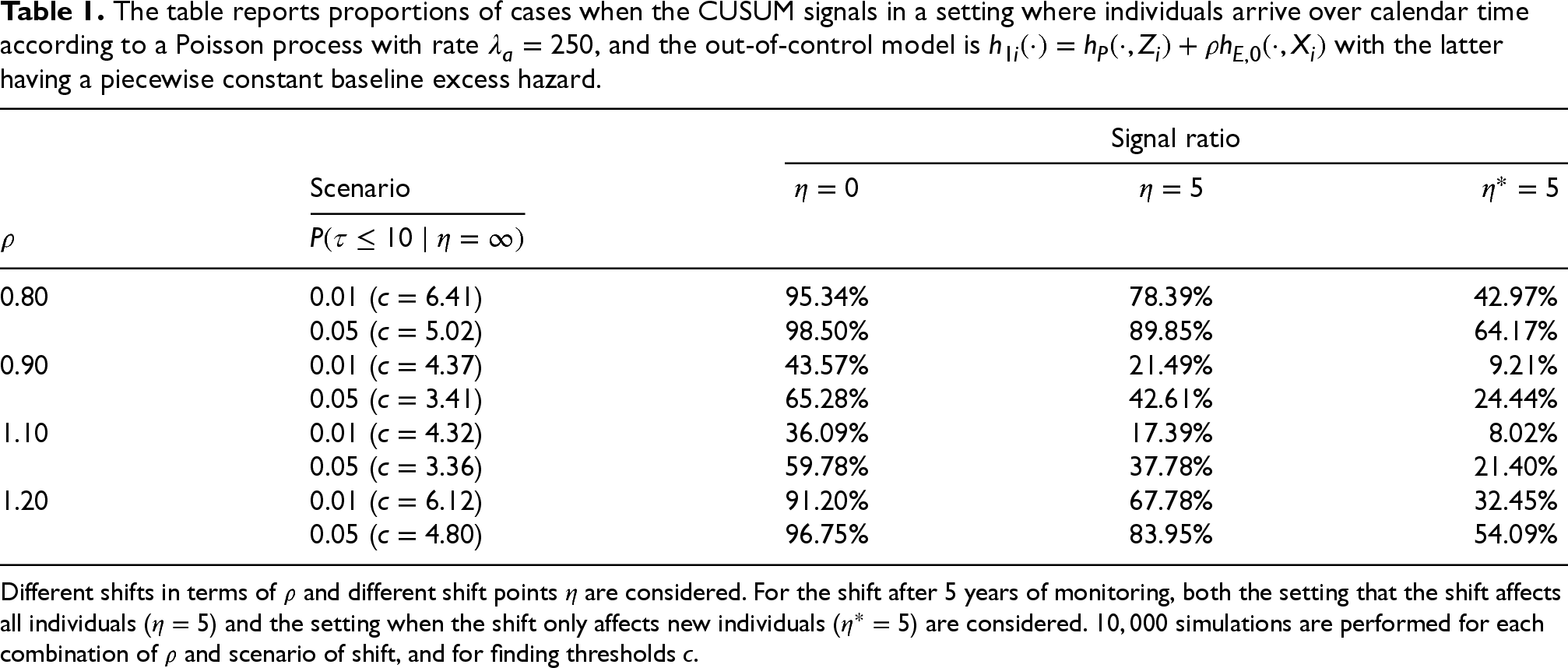
The table reports proportions of cases when the CUSUM signals in a setting where individuals arrive over calendar time according to a Poisson process with rate
, and the out-of-control model is
with the latter having a piecewise constant baseline excess hazard.
The table reports proportions of cases when the CUSUM signals in a setting where individuals arrive over calendar time according to a Poisson process with rate
Different shifts in terms of
The table reports proportions of cases when the CUSUM signals in a setting where individuals arrive over calendar time according to a Poisson process with rate
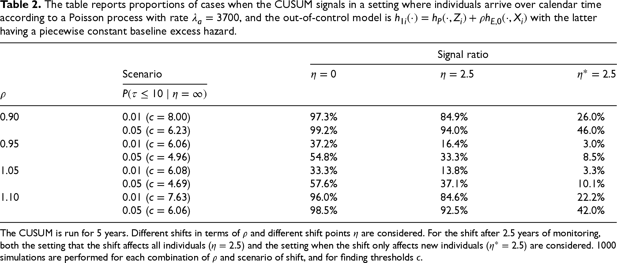
The CUSUM is run for 5 years. Different shifts in terms of
The table reports proportions of cases when the CUSUM signals in a setting where individuals arrive over calendar time according to a Poisson process with rate
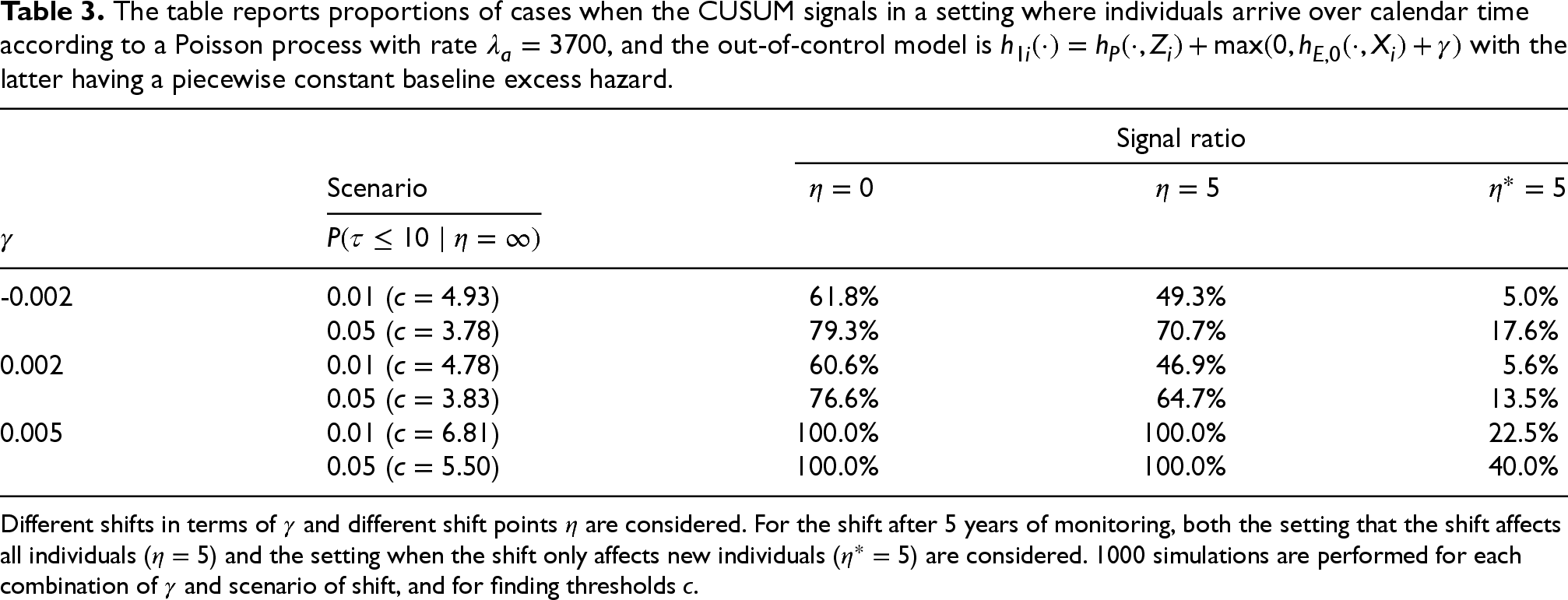
Different shifts in terms of
We study three different scenarios for the shift from in-control to out-of-control: (i) all patients are in the out-of-control situation from the beginning (
This subsection considers different scenarios with the proportional alternative represented by (2). The charts are computed using the correct value of
The results from the described simulation set-up are given in Table 1. One can observe that in the situation when the excess hazard is in the out-of-control state from the start, almost all simulations yield a signal during the 10-year monitoring period for the largest shifts, that is
Next, a situation with a much larger arrival rate, similar to what is observed in the cancer registry data used in Section 4, is considered by letting
Additive alternative
In this subsection, we perform a similar experiment as in the preceding for the additive alternative given by (3). By letting
Linear accelerated time alternative
For the last set-up in this section, we investigate the performance of the linear accelerated time alternative (5) with four different values of
The table reports proportions of cases when the CUSUM signals in a setting where individuals arrive over calendar time according to a Poisson process with rate
, and the out-of-control model is
with the latter having a piecewise constant baseline excess hazard.
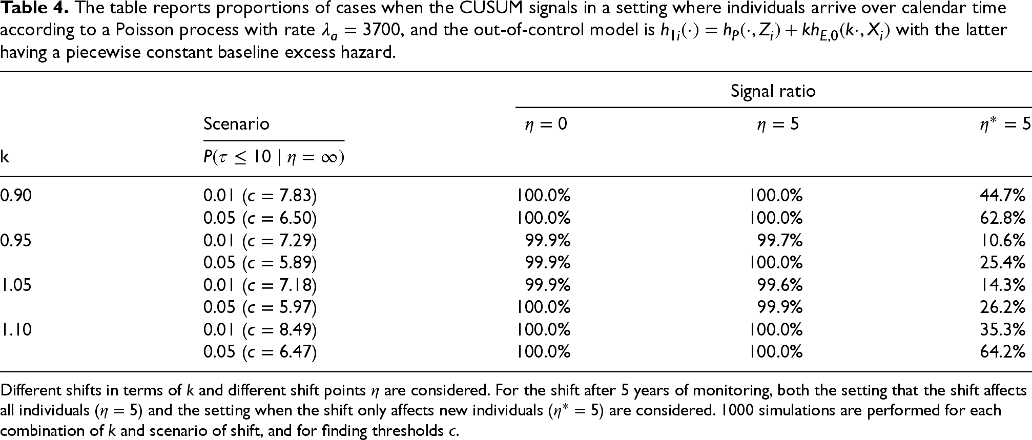
The table reports proportions of cases when the CUSUM signals in a setting where individuals arrive over calendar time according to a Poisson process with rate
Different shifts in terms of
In the preceding simulation studies, the true covariate parameters and functional form of the baseline excess hazard are used when computing the CUSUM charts. In practice, these are all unknown quantities and need to be estimated as discussed in Section 2.7. To illustrate the effect of estimation error in achieving, for example the specified in-control false probability or average run length, we perform the simulation set-up presented in Algorithm 2.
Furthermore, we will also consider some model misspecification aspects. One would presume that the observed in-control false signal probability will be further off from the nominal value if the specified form of the baseline is not correct, for example when using a piecewise constant baseline excess hazard model when the true excess hazard is a continuous function. Consequently, we will consider two different types of baseline excess hazard in this subsection: a piecewise constant baseline and a flexible smooth nonparametric baseline hazard. Both methods can be found in the R package
In addition, we also investigate for each combination of estimation procedure and true excess hazard if the results obtained from bootstrapping the covariate distributions from the data set obtained in step 2 of Algorithm 2 differ from simulating directly from the true covariate distributions. We will only perform the simulation using the proportional alternative, but the idea is the same for the remaining out-of-control situations.
Piecewise constant baseline
In this part of the simulation, we consider the same piecewise constant baseline excess hazard set-up presented previously in this section. The arrival rate is set to
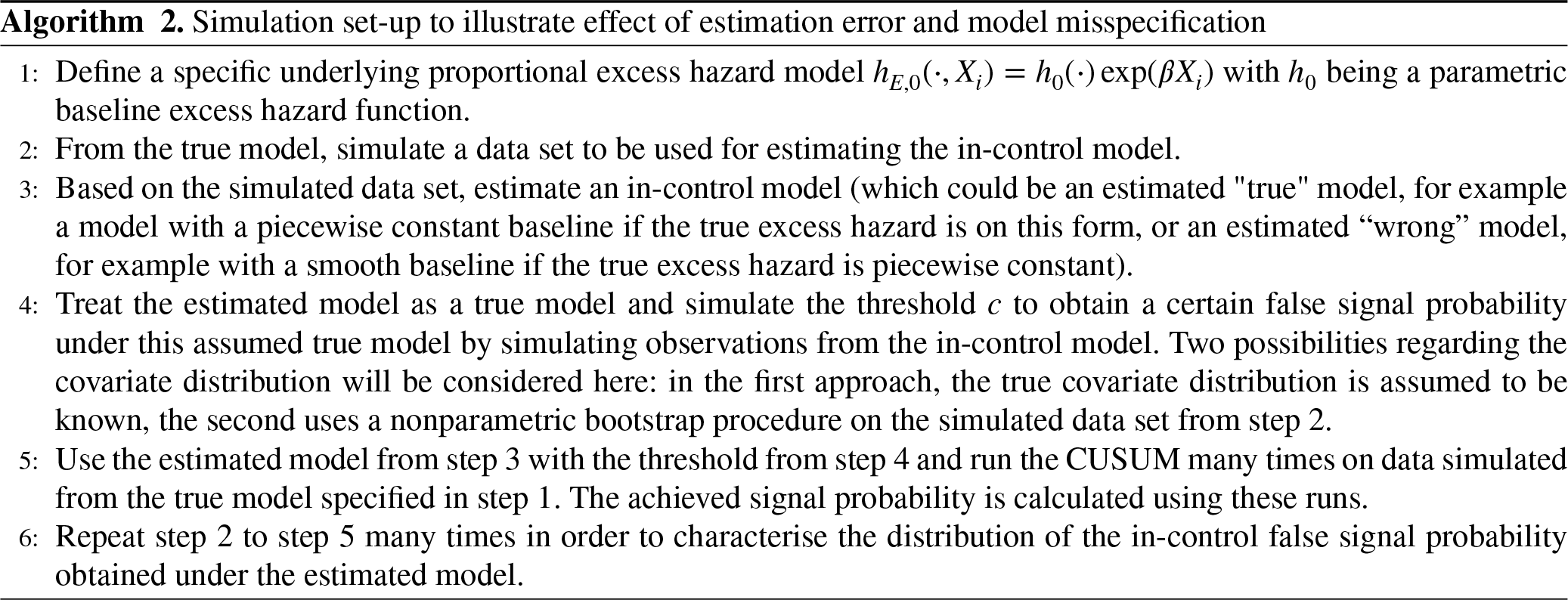
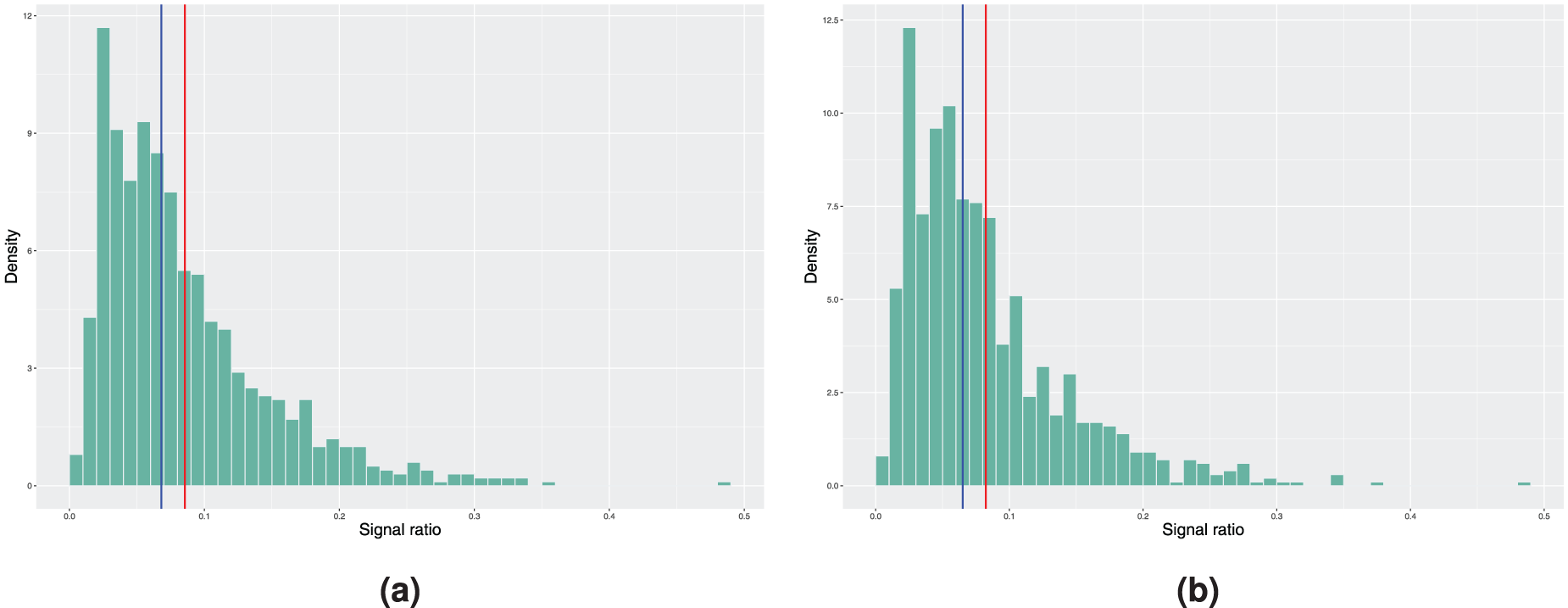
Histograms of the achieved signal probabilities under the in-control scenario with the true baseline excess hazard following a piecewise constant function. The model estimation is done using the model with piecewise constant baseline in step 3 of Algorithm 2. Here, the blue vertical line represents the median and the red line corresponds to the mean signal ratio. (a) True covariate distribution used in step 4 of Algorithm 2. Mean signal ratio is 5.73%, median signal ratio is 4.30% and (b) bootstrapping used to estimate the covariate distribution. Mean signal ratio is 5.65%, median signal ratio is 4.30%.
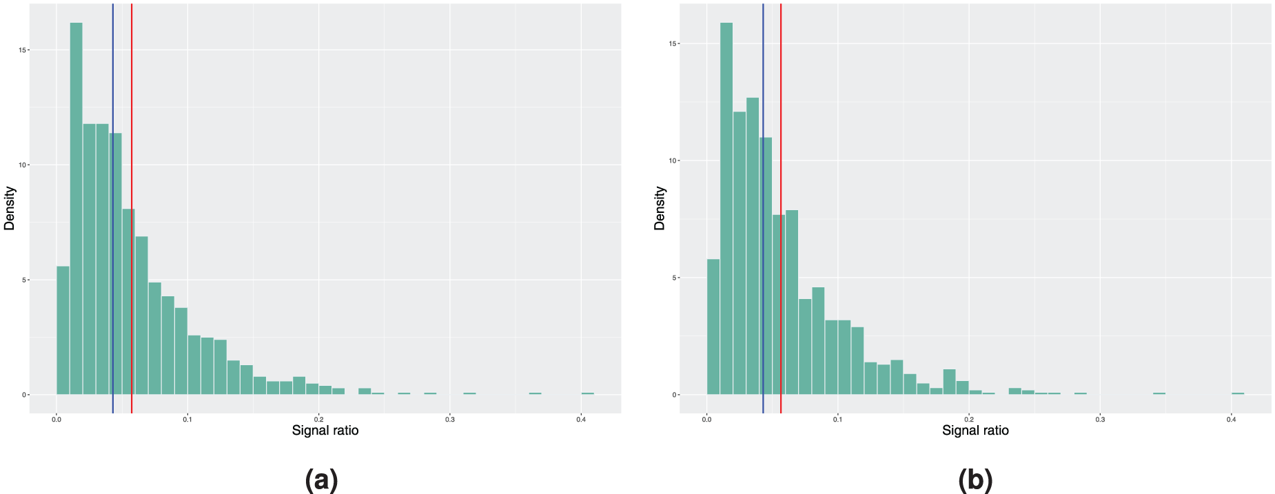
Histograms of the achieved signal probabilities under the in-control scenario with the true baseline excess hazard following a piecewise constant function. The model estimation is done using a smooth nonparametric baseline excess hazard in step 3 of Algorithm 2. Here, the blue vertical line represents the median and the red line corresponds to the mean signal ratio. (a) True covariate distribution used in step 4 of Algorithm 2. Mean signal ratio is 10.23%, median signal ratio is 8.20% and (b) bootstrapping used to estimate the covariate distribution. Mean signal ratio is 10.10%, median signal ratio is 8.10%.
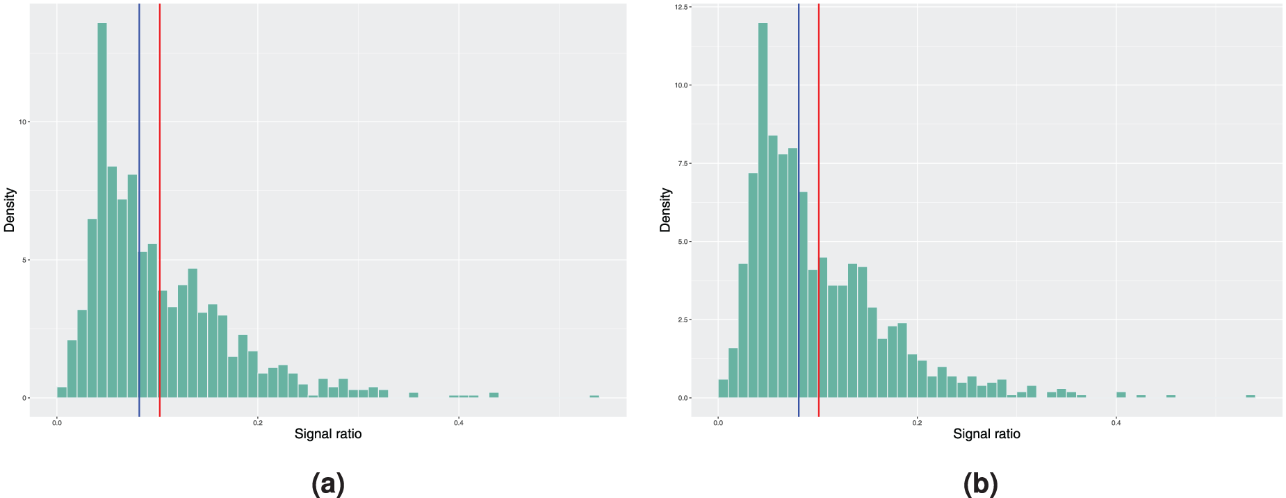
Histograms of the achieved signal probabilities under the in-control scenario with the true baseline excess hazard following the hazard function of the Weibull distribution. The model estimation is done using the model with piecewise constant baseline in step 3 of Algorithm 2. Here, the blue vertical line represents the median and the red line corresponds to the mean signal ratio. (a) True covariate distribution used in step 4 of Algorithm 2. Mean signal ratio is 4.14%, median signal ratio is 3.00% and (b) bootstrapping used to estimate the covariate distribution. Mean signal ratio is 4.09%, median signal ratio is 2.90%.
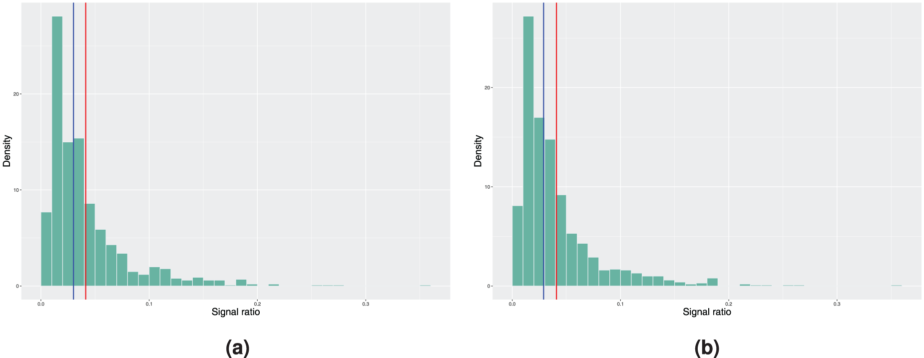
Histograms of the achieved signal probabilities under the in-control scenario with the true baseline excess hazard following the hazard function of the Weibull distribution. The model estimation is done using a smooth nonparametric baseline excess hazard in step 3 of Algorithm 2. Here, the blue vertical line represents the median and the red line corresponds to the mean signal ratio. (a) True covariate distribution used in step 4 of Algorithm 2. Mean signal ratio is 8.55%, median signal ratio is 6.80% and (b) bootstrapping used to estimate the covariate distribution. Mean signal ratio is 8.24%, median signal ratio is 6.50%.
On the other hand, when examining the results of the same procedure using the smooth baseline excess hazard estimate from Figure 2, we see that the median and mean in-control signal ratio, independent of the scenario considered in step 4 of Algorithm 2, are further away from the nominal value. Not only do we have the estimation error in the covariate parameters that affects the results, the incorrect specification of the form of the baseline excess hazard when using the smooth baseline estimate leads to larger deviation from the desired false signal ratio. Therefore, if the true baseline excess hazard is indeed a piecewise constant function, approximating it with a continuous and smooth function might cause undesired behaviour in the monitoring procedure.
In theory, the previous true form of baseline excess hazard favours the model with piecewise constant baseline as it is difficult for the estimated smoothed nonparametric baseline excess hazard to capture the stepwise behaviour. We now illustrate the opposite scenario by considering a Weibull baseline as the true form, where
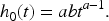
Figure 4 reports the results obtained when using the smooth nonparametric baseline excess hazard estimate. The in-control signal ratio obtained is slightly closer to the desired value of 5%, but the difference in absolute value is still larger compared to the piecewise constant model from above. We suspect that this is a consequence of the choice of the smoothing parameters in the experiment. This example shows a potential issue with the nonparametric baseline excess hazard estimate
2
- the smoothing parameters will have a large impact on how the charts will perform compared to the required in-control performance. An ideal situation is to obtain the full continuous estimate of
Application to colorectal cancer data monitoring
In this section, we apply the proposed methods to a data set of patients diagnosed with colorectal cancer in Norway between the start of 1970 and the end of 2020, followed up until the end of 2020. We will focus on patients with specified and known position of the tumour according to the International Classification of Diseases (ICD), who received standard surgical resections for cure of stage I–III colorectal cancer. With reference to Table A.1, this means that the relevant subset is the patients in surgery group 0, with SEER stage equal to localised or regional and with ICD indicator equal to 0, 1, or 2. Furthermore, while colorectal cancer is mostly a disease of the elderly, there has been a significant rise in incidence of this disease among the younger population, defined as early-onset colorectal cancer, that is
In this example, we explore monitoring in bands of 10 years, that is we choose a baseline period of 10 years and use the model fitted for this period to monitor for change during the next 10 years. This may provide important insight into the effects of new treatments and policy changes on outcomes for large patient populations on a macro health care level. More specifically, we define the first baseline period to be between 1970 and 1980. The patient cohort diagnosed in this period is used to fit an excess hazard model that will represent
In addition, only a piecewise constant baseline excess hazard model is considered here. The partition of the follow-up interval is in line with the simulation setups in Section 3, that is yearly bands for the first 5 years and then a last band from 5 to 10 years of follow-up. With these results as the in-control period, we run the CUSUM charts for the next 10 years, that is the time period between 1980 and 1990. Subsequently, this period is then used as the baseline period for the new monitoring period of 1990 to 2000, and this is done until we monitor the period between 2010 and 2020.
For each period, we will for illustration purposes run several charts corresponding to monitoring for different degrees of improvement or worsening from the in-control baseline excess hazard. In terms of the interpretation of the method, the CUSUM charts for the period between 1980 and 1990 will signal if there is accumulation of evidence in the data of improvement or worsening, depending on the specified alternative, with respect to the baseline time period between 1970 and 1980. Similarly, the charts for the period between 1990 and 2000 will signal if there is accumulated evidence of a change in the excess hazard from the baseline period of 1980 and 1990, and so on.
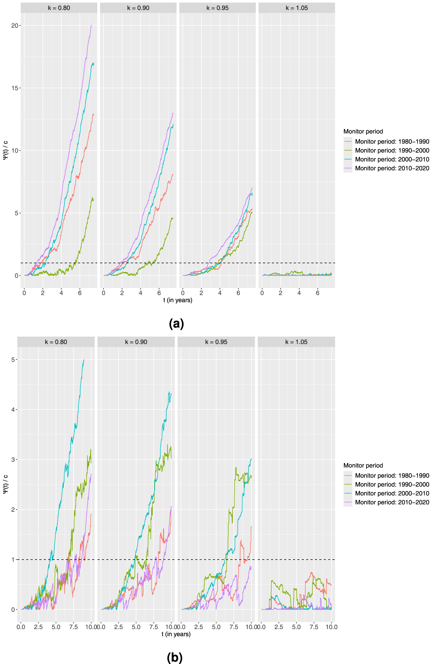
Proportional alternative
First, we consider the proportional alternative. For each combination of age group and monitoring period, the chart is computed using four different values of
Standardised CUSUM charts using the proportional alternative for each age group monitoring 10-year survival in four different time periods with the estimated output from the piecewise constant baseline excess hazard model fitted on the preceding 10-year time period as the in-control. Four different values of
It is clear from both plots that the charts fluctuate and do not signal for any combinations of age group and time period when considering the increased burden of disease scenario of
An explanation for this could be that no advances in treatment compared to the 1980s were observed during the first half of the 1990s. On the other hand, the chart signals fastest in the period 2010 to 2020. This could indicate early advances in this period, but the faster signal could also possibly be partly explained by more patients arriving during this time interval. For the younger, there seems to be an indication of a better treatment advance in the period 2000 to 2010 versus the previous decade than in the other periods. The generally later signals for the younger could be explained by much fewer patients in this group.
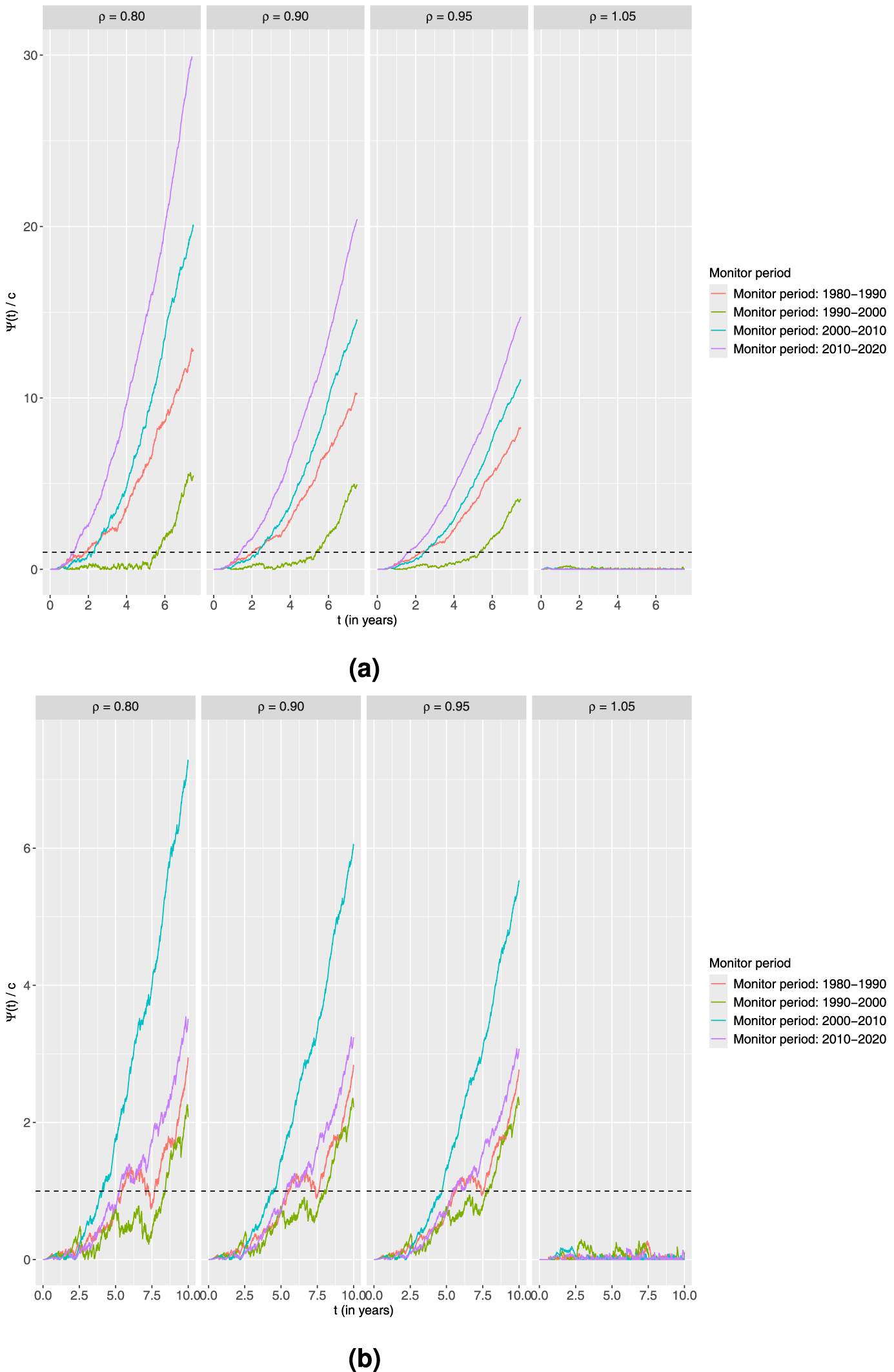
Next, we investigate the setting of an additive alternative. As in the previous setting, we also here use three shift parameters that correspond to decreasing and one corresponding to increasing excess hazard, that is the values of
Standardised CUSUM charts using the additive alternative for each age group monitoring 10-year survival in four different time periods with the estimated output from the piecewise constant baseline excess hazard model fitted on the preceding 10-year time period as the in-control.
Standardised CUSUM charts using the linear accelerated time alternative for each age group monitoring 10-year survival in four different time periods with the estimated output from the piecewise constant baseline excess hazard model fitted on the preceding 10-year time period as the in-control.
For the remaining values of
Looking at the charts obtained from the younger age group, no signals are now obtained in the first two monitoring periods for
Finally, we try a linear accelerated time alternative with the following four values of the acceleration parameter
The most interesting observation from the results presented in Figure 7 regarding the younger age group is the charts corresponding to the periods 1990 to 2000 and 2010 to 2020. With the additive alternative, the charts monitoring towards improvement for 1990 to 2000 did not signal at all. However, with the linear accelerated time alternative, all charts for this period signal for all values of
Summary
We have presented a CUSUM-based method for monitoring changes in excess hazard for relative survival settings where the population hazard is known. This complements the literature on monitoring based on time-to-event models. The proposed method can be used for real-time monitoring, semi real-time monitoring or for retrospective analyses. The method can be adapted to various data updating schemes.
We have considered proportional, additive and linear accelerated time change models and studied properties by simulations and in an application to cancer registry data. In particular, we have also considered the impact of estimation error and some forms of model misspecifications. Simulations indicate that model misspecifications might be a somewhat severe issue, while with a decent amount of baseline data the impact of estimation error is not so critical. To our knowledge, there is no formal testing procedure available to test the functional form of the baseline excess hazard. Fortunately, the deviations observed in the simulations are smallest in the situation that will most likely appear in practice where the true baseline hazard function is continuous and the fitted model is piecewise constant.
Furthermore, we have mainly focused on monitoring using proportional excess hazard models. For some cancer types, it is known that the excess hazard is not proportional. In contrast to the scenario related to misspecification of the baseline hazard, checking and performing formal hypothesis test for violation of this assumption can be done using Schoenfeld-like residuals proposed by Stare et al. 25 or martingale residuals proposed by Danieli et al. 26 The latter residuals can also be used to check the validity of the functional form of the covariates in the model. 26
For small sample sizes, the bootstrap approach for handling estimation error presented in Gandy and Kvaløy 27 could in principle be adapted, although with a substantial computational burden in the current setting. Applications to data illustrate that careful considerations need to be made when specifying the type of changes in the excess hazard to monitor against.
For the scenarios considered in this paper, year of diagnosis or variants of time with respect to the start of monitoring is not included as a predictor. However, one could fit a model where year of diagnosis is included as predictor to model a general secular trend, assume that this trend continues into the monitoring period, and use the proposed method to monitor drift from the secular trend.
Another extension that could be considered is to try to extend the approach to cure models, for instance by trying to adapt the CUSUM for cure models presented by Oliveira et al. 11 to the excess hazard setting. Here, this would correspond to some individuals having zero excess hazard. A different variant would be cure models where all individuals have zero excess hazard after some cure time point, this should work automatically with the current set-up if a proportional alternative is used.
Finally, it could be of interest to avoid the requirement of specifying a specific alternative in order to capture more general out-of-control situations. Phinikettos and Gandy 28 have proposed a method that avoids this necessity for the setting of non-risk-adjusted total hazard monitoring. Extending this methodology to the relative survival situation of interest here, but also allowing for the incorporation of covariates via regression models, could be an interesting direction in the future.
Footnotes
Acknowledgments
The authors would like to thank the three anonymous referees for detailed and helpful feedback that led to an improved manuscript. The authors would also like to express gratitude to Professor Axel Gandy for helpful comments regarding the manuscript and interesting suggestions that have been partly mentioned in the discussion.
Ethical approval and informed consent statements
Ethical approval was provided by the Regional Committee for Medical and Health Research Ethics, Western Norway (Ref. no. 343976). The data set was anonymised according to the guidelines from the Norwegian Data Protection Authority. Exemption from confidentiality was provided by the National Institute of Public Health.
Funding
The authors disclosed receipt of the following financial support for the research, authorship, and/or publication of this article: Jimmy Huy Tran acknowledges finanacial support by Finansmarkedsfondet (Grant Number: 337601).
Declaration of conflicting interest
The authors declared no potential conflicts of interest with respect to the research, authorship, and/or publication of this article.
Disclaimer
The study has used data from the Cancer Registry of Norway. The interpretation and reporting of these data are the sole responsibility of the authors, and no endorsement by the Cancer Registry of Norway is intended nor should be inferred.
A. Summary table of the covariates in the simulation set-up of Section 3
Overview of the covariates used in the simulations, with the corresponding parameter value used and proportion of observations simulated to be in each category for the categorical covariates. Age is simulated from a normal distribution with mean 75 and standard deviation 10, truncated at 50 and 105. See Tran 23 for details about the medical interpretations of the covariates.
| Variable |
|
Proportion |
|---|---|---|
| Gender Male | 50.00% | |
| Gender Female | 50.00% | |
| ICD indicator 0 (Rectum) | 27.00% | |
| ICD indicator 1 (Right colon or appendix) | 44.00% | |
| ICD indicator 2 (Left colon) | 28.00% | |
| ICD indicator 3 (Unspecified location or colon polyps) | 1.00% | |
| Morphology type Adenocarcinoma | 90.00% | |
| Morphology type Mucinous carcinoma | 10.00% | |
| SEER stage Distant | 20.00% | |
| SEER stage Localised | 20.00% | |
| SEER stage Regional | 55.00% | |
| SEER stage Unknown | 5.00% | |
| Surgery group 0 (Major surgery) | 82.75% | |
| Surgery group 1 (Minor surgery) | 17.15% | |
| Surgery group 2 (No surgery) | 0.10% |
B. Smoothing procedure for the semiparametric excess hazard model in the CUSUM method
An important note regarding the semiparametric excess hazard model implemented in the R package