
Abstract
Simultaneous confidence intervals that are compatible with a given closed test procedure are often non-informative. More precisely, for a one-sided null hypothesis, the bound of the simultaneous confidence interval can stick to the border of the null hypothesis, irrespective of how far the point estimate deviates from the null hypothesis. This has been illustrated for the Bonferroni-Holm and fall-back procedures, for which alternative simultaneous confidence intervals have been suggested, that are free of this deficiency. These informative simultaneous confidence intervals are not fully compatible with the initial multiple test, but are close to it and hence provide similar power advantages. They provide a multiple hypothesis test with strong family wise error rate control that can be used in replacement of the initial multiple test. The current paper extends previous work for informative simultaneous confidence intervals to graphical test procedures. The information gained from the newly suggested simultaneous confidence intervals is shown to be always increasing with increasing evidence against a null hypothesis. The new simultaneous confidence intervals provide a compromise between information gain and the goal to reject as many hypotheses as possible. The simultaneous confidence intervals are defined via a family of dual graphs and the projection method. A simple iterative algorithm for the computation of the intervals is provided. A simulation study illustrates the results for a complex graphical test procedure.
Keywords
Introduction
Informative simultaneous confidence intervals (iSCIs)
Numerous multiple comparison procedures are available for a large spectrum of settings, where more than one confirmatory assertion is desired so that the familywise error rate is controlled in the strong sense (see e.g. Hochberg and Tamhane 1 or Dickhaus 2 for an overview). Because of the increasing importance in practice, a (draft of the) EMA/CHMP Guideline on multiplicity issues in clinical trials 3 has been published. Besides error control, it emphasizes the importance of obtaining clinically interpretable results by providing confidence intervals that “allow for consistent decision making with the primary hypothesis testing strategy.” The implementation of such a decision strategy is impeded by the fact that simultaneous confidence intervals (SCIs), which are both compatible with a given multiple test, and informative, are not easy to find. Compatibility means that a null hypothesis is rejected if and only if it is excluded from the confidence interval.
We will call a confidence interval informative, if the information provided by the interval always increases (and only stays constant in the case that all gatekeepers for a hypothesis were not rejected) with increasing evidence against the corresponding null hypothesis. As a consequence, when a null hypothesis is rejected, the confidence interval will have a non-zero distance to the null hypotheses, except for the singular and usually negligible event that the corresponding (un-adjusted) p-value is equal to its final local level. Hence, informative confidence intervals almost always provide additional information to the mere hypothesis test.
To be more formal, let us consider
We call a SCI given by lower bounds for all
The restriction in (a) of Definition 1 corresponds to the case where rejection of a hypothesis Note, that in the case where for both data sets We have intentionally left point (b) in Definition 1 somewhat informal, namely with regard to meaning of the statement “increasing evidence against Let us assume that the evidence against We will see (and explicitly state) below that for our method and theory to apply, we need the existence of p-values The property, that
Strassburger and Bretz
7
and Guilbaud8,9 have proposed SCIs for a large class of stepwise procedures. These SCIs are not always informative, for example, if not all hypotheses are rejected then the confidence intervals of rejected hypotheses equal the whole alternative hypotheses, irrespective of how much the point estimate points into the alternative hypothesis. Hence, they contradict Definition 1 and they are only of limited use, because they do not provide any more information than the rejection itself. Guilbaud
10
proposes SCIs that can be more informative than the rejection itself in certain scenarios for some of the hypotheses studied. However, they also do not meet Definition 1. The recommendation of the (draft of the) EMA Guideline on multiplicity issues in clinical trials concerning this conflict of interest is the following: “it is advised to use simple but conservative confidence interval methods, such as Bonferroni-corrected intervals.” This is comprehensive with regard to the wish of having intervals that do not lead to misinterpretation, which is of greatest importance in practice. On the other hand, there is the need for a compromise, because the recommended intervals are either compatible with the—conservative—hypothesis test, or informative but not compatible with a more complex test. Since SCIs contain always more information than pure rejection decisions, a natural way out of this conflict is to construct the multiple testing procedure by directly defining informative simultaneous confidence bounds
Based on this idea, Brannath and Schmidt
4
have constructed informative SCIs, which are always informative and uniformly more powerful than the Bonferroni procedure with regard to the number of rejected hypotheses. They can be seen as a compromise between the powerful Bonferroni-Holm procedure and the informative Bonferroni procedure. Similar procedures were proposed for the hierarchical and the fallback test by Schmidt and Brannath.5,6 All these procedures belong to the class of graphical test procedures introduced by Bretz et al.
11
which permit to account for preferences and hierarchies among the different null hypotheses
In the following subsection, we will recall the definition of the graphical procedures from Bretz et al., 11 which sets the basic notation for the new approach. In Section 2, we introduce the new SCIs, first by a formal definition, which motivates the approach, and subsequently by an iterative algorithm, which can be implemented numerically. We will see that both perspectives yield the same SCIs. In Section 3, we link the extended setting to our previous SCIs proposed for the hierarchical, fallback, and Bonferroni-Holm procedure (Brannath and Schmidt, 2014; Schmidt and Brannath, 2014, 2015), and we give an example of a more complex graph where the advantages of the new approach are demonstrated. We conclude with a discussion in Section 4.
A multiple testing procedure by Bretz et al.
11
is given by a graph initial local levels a transition matrix
An example is given in Figure 1. This graph is given by Bretz et al.
11
and is an example for a step-down test without order constraint from Bauer et al.
12
Three treatments are compared with respect to efficacy and safety so that altogether six hypotheses are tested. The significance level is equally split across the three efficacy hypotheses, that is,
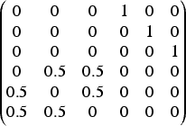
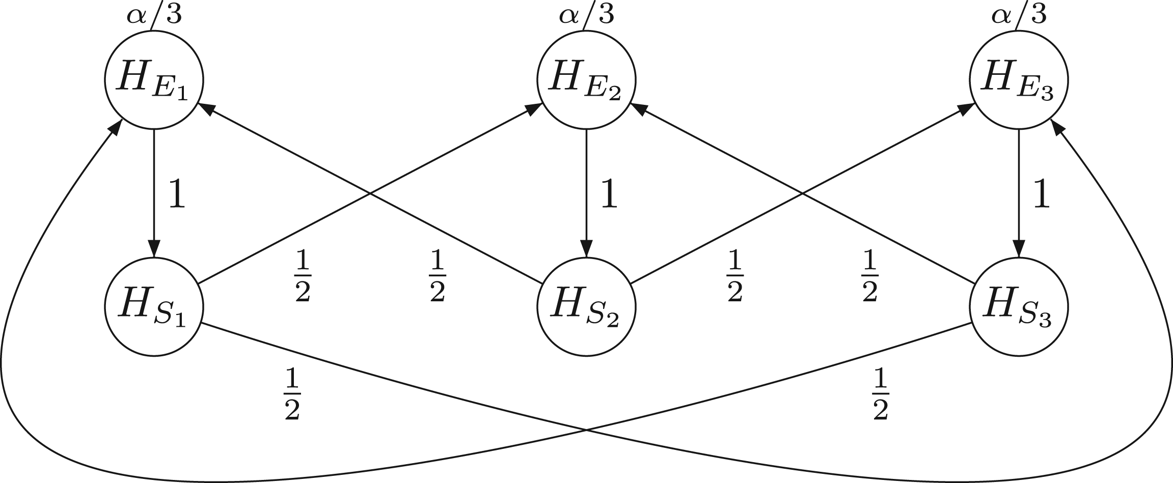
Example for a complex graphical procedure (Figure 8 from Bretz et al., 2009).
The graphical algorithm is as follows: If a hypothesis
Definition of confidence bounds
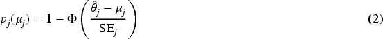
Given observations (e.g. from a clinical trial), we assume that we have local p-values
Our starting point is a graph like the one given in Section 1.2, that is, we have initial levels
We assume that for all
We will explain in Remark 8 how our procedure can be adapted if the graph is not complete.
Basic projection method
By modifying the given graph, we construct weighted Bonferroni tests for the intersection of shifted hypotheses
We next construct the simultaneous confidence bounds
Dual graphs and resulting weighted Bonferroni tests
For each
For given
First step. We define a new graph for all delete all paths starting at replace for all add a node for the hypothesis introduce an arrow from change all transition weights starting from
The resulting graph
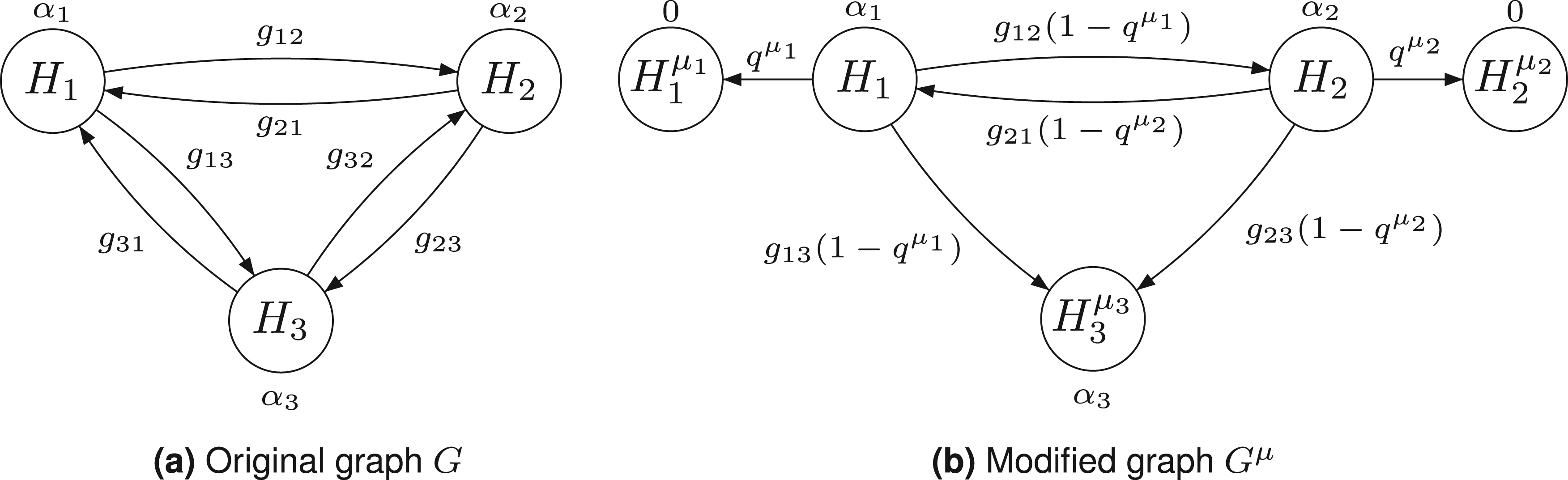
From the original graph (a) to a graph (b), where the shifted hypotheses
The rationale for the graph
Second step. We reject in
According to the projection method described at the beginning of this section, the new lower simultaneous confidence bounds are then defined as follows.
Given the p-values

We now prove a property of the local levels
For all
We know or can see from Bretz et al.
11
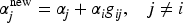
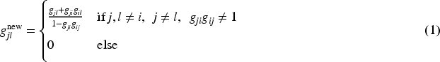
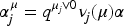
and the up-date algorithm therein that the graphical test algorithm has the following properties: The order in which hypotheses are rejected does not influence the local levels of the final graph. After every rejection step, the new transition weights are continuous and non-decreasing functions of the old transition weights. After every rejection step, the new level of a hypothesis and the new weights starting from this hypothesis are independent of the old levels of any other, non-rejected hypothesis and independent of all old transition weights that go from or to the other, non-rejected hypotheses. The new level of a hypothesis is a linear combination of
Fix
If
We remind that

Note that both, the left-hand side and the right-hand side of (5), are non-decreasing in
Find a starting vector


By continuity and monotonicity, the first iterated value
Our next goal is to show that
The following properties are satisfied in Algorithm 1: If The limiting value is independent of the starting value of the algorithm. For any given starting value
We obtain from
As a starting value
Properties of the confidence bounds
The main property of the new confidence bounds is that they are always informative in the sense of Definition 1. This is an essential advantage over the SCIs proposed by Strassburger and Bretz. 7
The simultaneous confidence bounds obtained by Algorithm
We start showing (a) of Definition 1. As discussed in Remark 6, there exists a starting value
If
We consider now property (b). Let
To assure the informativeness of the SCIs, we pay a price in terms of a slightly reduced expected number of rejections to the underlying original graphical procedure. We can, however, control the desired power by the choice of the information weight
One can also generalize the approach by choosing individual information weights
Assumption 1 can be weakened so that the approach is also applicable for graphical procedures with non-complete graphs. We only need to adapt the transition weights in
Alternatively to this modification, one could of course also add arrows in the original graph so that Assumption 1 is satisfied. This can be done if one wants to increase power for certain hypotheses rather than improve confidence assertions. However, the latter is not always possible, for example, in hierarchical testing.
Bonferroni-Holm procedure
The graph in Figure 2(a) represents the weighted Bonferroni-Holm procedure for three hypotheses. If
The same features hold for the approach of penalized SCIs introduced by Schmidt and Brannath
4
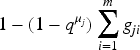
where attention is restricted to the unweighted Holm procedure and specific union intersection tests. The penalized SCIs for the Holm test are constructed via dual weighted Bonferroni tests, where the weights are based on a so-called “penalization function.” The penalization function
The scenario of the simulation is the following: five null hypotheses (e.g. the effects of different treatments compared to placebo) are tested with equal weights. We assume a scenario where all true effects are equally large. Other scenarios led to similar results. The significance level is
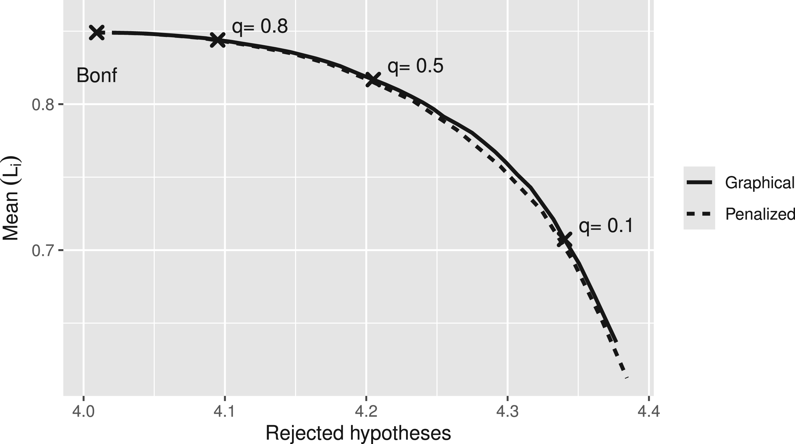
Trade-off between mean confidence bound
According to Schmidt and Brannath,5,6 we have introduced iSCIs for the hierarchical and the fallback procedure, respectively. We show in the Appendix that Algorithm 1 produces exactly the same SCIs. We have discussed properties of these SCIs in our previous works. In particular, the SCIs are always informative. This holds for all graphical iSCIs, as we have shown in Proposition 7. The case of gatekeepers discussed in Definition 1 and Remark 6 is of particular relevance for the fixed sequence: If some
A nice feature of the iSCIs is that they somehow respect the ordering in the hierarchical and the fallback procedure, in the sense that there is no power loss compared to the original procedure for the first hypothesis, which is normally the most important one. The price that has to be paid for more information is a slight power loss for
A clinical trial example
We consider now a hypothetical clinical trial example that is in line with the RELY trial, reported by Connolly et al. 13 In this trial, two doses of the thrombin inhibitor dabigatran were compared to warfarin (active control) in a randomized and semi-blinded, multi-arm clinical trial. The primary treatment goal is the risk reduction of strokes or systematic embolisms in patients with atrial fibrillation. There are a primary efficacy and a safety parameter (both hazard ratios). The data indicated that the lower dabigatran dose is non-inferior and the higher dose even superior to warfarin with regard to efficacy (i.e. hazard for a stroke or systematic embolism), and that the low dabigatran dose seems to be superior to warfarin with regard to safety (hazard for major bleeding). Since the multiplicity adjustments anticipated in the trial were only with regard to the two non-inferiority null hypotheses in efficacy, superiority claims with regard to efficacy and claims on safety are not strictly confirmative. iSCIs based on as graph as shown in Figure 1, but with two doses instead of three, permits strictly confirmative claims also with regard to superiority in the efficacy and safety endpoints. We will illustrate below how the study could have been planned to include such a procedure. We will assume, for simplicity, that for the estimates for efficacy and safety are normally distributed with known standard errors (which is in line with the common asymptotic approximation for the log-hazard rates).
As indicated in Figure 1, effectiveness of the doses is primarily tested by non-inferiority. Accordingly, the hypotheses are
Of course, it would be valuable to also show superiority over the active comparator for the efficacy endpoint if the effect estimate is large. To this end, the simultaneous confidence bounds would need to be informative, such that
Trial planning
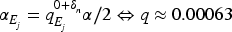
We now discuss how the trial could have been planned with our iSCIs. To this end, we fix the one-sided overall level
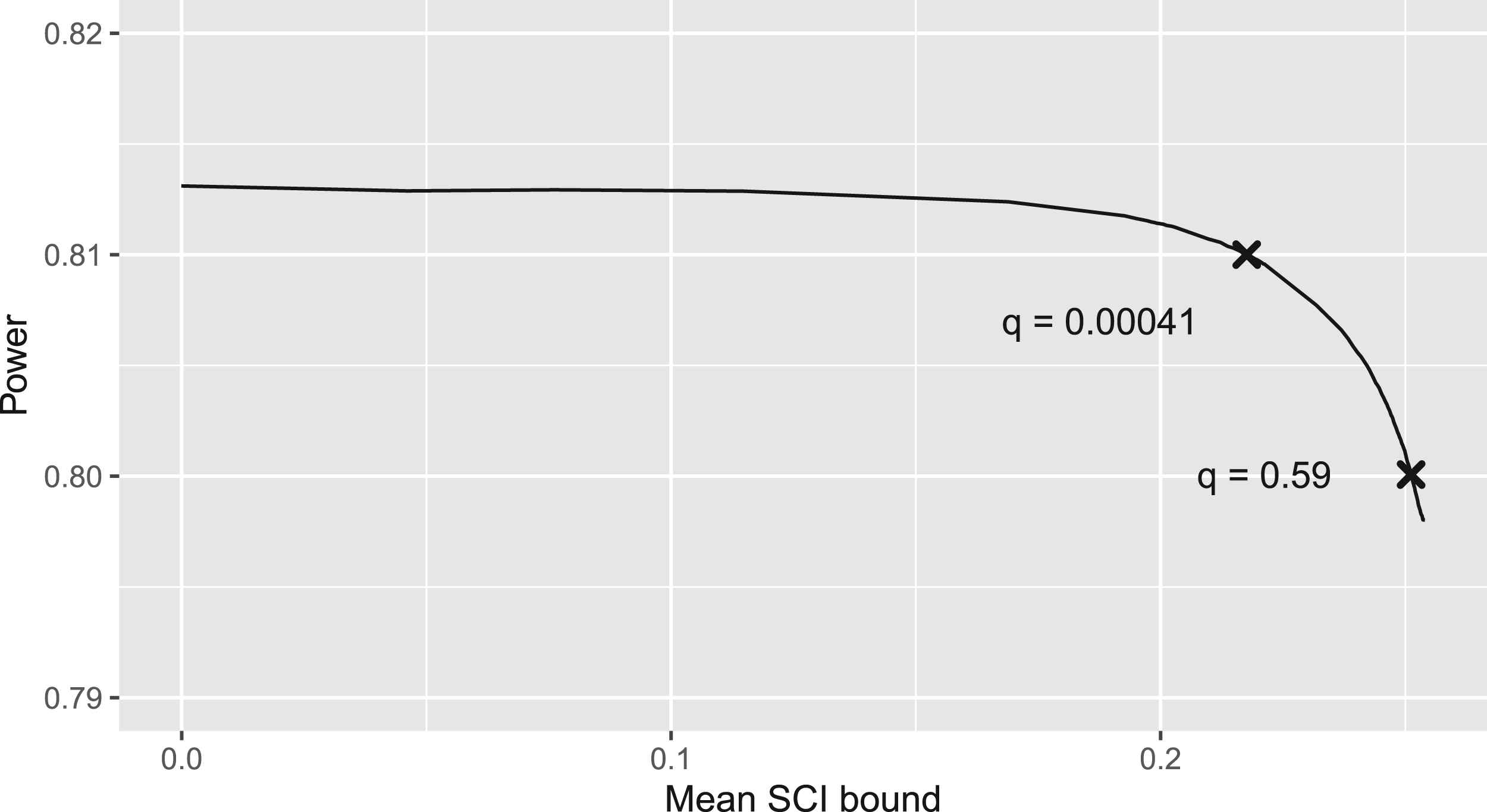
Probability to reject
For the simulation, we used our developed
From the simulation results, we can do the trade-off between higher power and higher information of the SCIs. For example, we could choose that value of the information weight
As a next step we want to apply the proposed method to calculate iSCIs to the data reported by Connolly et al.
13
The calculation of the iiSCIs can be done with our
We can see that with the cSCIs, the two non-inferiority hypothesis for the efficacy endpoints
While in this setup one-sided SCIs are sufficient to answer the trial question, in many trials, two-sided intervals are desired. Since there is no hierarchy amongst the hypotheses regarding the upper limits in our example, we use Bonferroni-adjusted SCIs to derive upper limits. These are then intersected with the iSCIs to obtain two-sided intervals. This approach gives the following two-sided 95% SCIs: (
Comparison of the compatible and informative lower 97.5% SCI bounds on the RELY data.
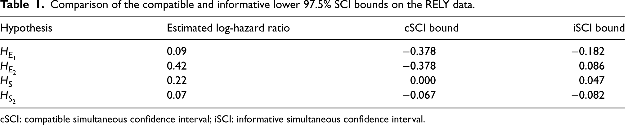
Comparison of the compatible and informative lower 97.5% SCI bounds on the RELY data.
cSCI: compatible simultaneous confidence interval; iSCI: informative simultaneous confidence interval.
The approach of informative graphical SCIs proposes a way out of the conflict between wishing to reject as many hypotheses as possible and at the same time obtaining relevant information on the parameters of interest by confidence intervals. The SCIs can be constructed for all graphical procedures from Bretz et al.
11
and will always give more information than the pure (non-)rejection of the hypotheses, except in the case where gatekeepers are not rejected and thus the hypothesis test and interval estimation of the parameter is considered to be of no interest. As usual, there is no gain without costs. Compared to the original graphical procedures, the iSCIs usually pay a price in terms of rejections. The possibility to adapt the SCIs to trial specific priorities concerning information and/or power is via the choice of the information weight
Extension to
-graphs
So far, we have not explicitly considered graphs that use the
Extension to group sequential designs
It is straightforward to extend the SCIs presented in this article to group sequential designs (GSDs). This can be done, for example, by splitting the total level alpha across the stages of the GSD and calculate the boundaries in each stage based on the new stage-wise level. Valid simultaneous confidence bounds can then be obtained for each parameter, by taking the maximum of the stage-wise bounds. While this procedure will produce valid SCIs it does not take into account the correlation of the stage-wise tests statistics for the individual hypotheses and might therefore leave room for improvement.
Restrictions and outlook
As we have seen in Section 3.1, the new method is more flexible than the penalized intervals from Brannath and Schmidt 4 in that all graphical procedures of Bretz et al. 11 can be adapted to informative graphical SCIs. However, it has to be recognized that an advantage of our previous approach was that it could be generalized to other step-down tests like the Dunnett procedure, which accounts for correlations between the test statistics and thus gains in power. A future aspect of work may, therefore, be to incorporate correlations also in the informative graphical SCIs, similar to the work of Bretz et al. 15 for the graphical procedure.
Supplemental Material
sj-R-1-smm-10.1177_09622802251393666 - Supplemental material for Informative simultaneous confidence intervals for graphical test procedures
Supplemental material, sj-R-1-smm-10.1177_09622802251393666 for Informative simultaneous confidence intervals for graphical test procedures by Werner Brannath, Liane Kluge and Martin Scharpenberg in Statistical Methods in Medical Research
Footnotes
Acknowledgements
We thank Serhat Günay for his help in the development of R programs for our simulation study. This research was supported by the DFG, grant BR 3737/1-1.
Funding
The author(s) disclosed receipt of the following financial support for the research, authorship, and/or publication of this article: The authors gratefully acknowledge the support of the Leibniz Science Campus Bremen Digital Public Health (www.digital-public-health.de), which is jointly funded by the Leibniz Association (W72/2022), the Federal State of Bremen, and the Leibniz Institute for Prevention Research and Epidemiology – BIPS.
Declaration of conflicting interest
The authors declared no potential conflicts of interest with respect to the research, authorship, and/or publication of this article.
Supplemental material
Supplemental material for this article is available online.
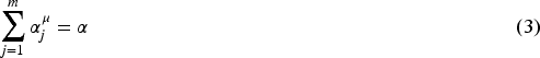
Appendix A. Proof of (3)
We will explain that (3) holds for any starting graph
In the modified graph
References
Supplementary Material
Please find the following supplemental material available below.
For Open Access articles published under a Creative Commons License, all supplemental material carries the same license as the article it is associated with.
For non-Open Access articles published, all supplemental material carries a non-exclusive license, and permission requests for re-use of supplemental material or any part of supplemental material shall be sent directly to the copyright owner as specified in the copyright notice associated with the article.